Wave Number of Maximal Growth in Viscous Magnetic Fluids of Arbitrary Depth

Abstract

An analytical method within the frame of linear stability theory is presented for the normal field instability in magnetic fluids. It allows to calculate the maximal growth rate and the corresponding wave number for any combination of thickness and viscosity of the fluid. Applying this method to magnetic fluids of finite depth, these results are quantitatively compared to the wave number of the transient pattern observed experimentally after a jump–like increase of the field. The wave number grows linearly with increasing induction where the theoretical and the experimental data agree well. Thereby a long-standing controversy about the behaviour of the wave number above the critical magnetic field is tackled.

I Introduction

Spontaneous pattern formation from a homogeneous ground state has been studied extensively in many nonlinear dissipative systems. Among these systems magnetic fluids have experienced a renewed interest in recent years due to their technological importance [1]. The most striking phenomenon of pattern formation in magnetic fluids is the Rosensweig or normal field instability [2, 3, 4, 5]. Above a threshold $B_{c}$ of the induction the initially flat surface exhibits a stationary hexagonal pattern of peaks. Typically, patterns are characterized by a wave vector ${\bf q}$ whose absolute value gives the wave number $q=|{\bf q}|$. In contrast to many other systems, a comprehensive quantitative theoretical and experimental analysis of the dependence of the wave number on the strength of the magnetic field is lacking for the normal field instability. There are few but contradictory experimental observations. In experiments where the field is increased continuously, there are reports about constant [2, 6] as well as about varying wave numbers [7] as the induction is increased beyond the critical value $B_{c}$. Notably, all these observations are of entirely qualitative character [8].

A first theoretical analysis leading to constant wave numbers of maximal growth was presented in [9]. The general dispersion relation for surface waves on a magnetic fluid of infinite thickness was analysed for two asymptotic regimes: for the inviscid regime and for the viscous-dominated regime. The main result for the latter regime was that taking into account viscous effects the wave number of maximal growth is the same at and beyond the critical induction. As will be shown below, this argument is rather misleading because realistic fluid properties are not covered by such an asymptotic analysis. The two asymptotic regimes in [9] were combined with very thin as well as very thick layers of magnetic fluid and the resulting four regimes were analysed in [11]. In three regimes a non-constant wave number of maximal growth was found.

All qualitative observations in [2, 6, 7] are referring to the final arrangement of peaks. The final stable pattern, resulting from nonlinear interactions, does not generally correspond to the most unstable linear pattern. Such a pattern should grow with the maximal growth rate and should display the corresponding wave number. Since both quantities are calculated by the linear theory, the most unstable linear pattern has to be detected and measured experimentally for a meaningful comparison between theory and experiment. No measurements of the most linear unstable pattern have yet been undertaken.

Motivated by this puzzling situation, the paper presents a quantitative theoretical analysis of the wave number with maximal growth rate for any combination of fluid parameters. Experimental measurements of the most linear unstable pattern are conducted and the data compared with the theoretical results. The system and the relevant equations of the problem are displayed in the next Section. Based on the dispersion relation from a linear stability analysis, an analytical method is presented to calculate $q_{m}$ and the maximal growth rate $\omega_{m}$ for any combination of material parameters. The details of the method are explained for a magnetic fluid of infinite thickness and the results are compared with previous asymptotic results (Sec. III). The method is also applied to magnetic fluids of finite thickness (Sec. IV), which allows a quantitative comparison with the experimental data (Sec. V). In the final section the results are summarized and further prospects are outlined.

II System and Equations of the Problem

A horizontally unbounded layer of an incompressible, nonconducting, and viscous magnetic fluid of thickness $h$ and constant density $\rho$ is considered. The fluid is bounded from below ($z=-h$) by the bottom of a container made of a magnetically impermeable material and has a free surface described by $z=\zeta(x,y,t)$ with air above. The electrically insulating fluid justifies the stationary form of the Maxwell equations which reduce to the Laplace equation for the magnetic potentials $\Phi^{(i)}$ in each of the three different regions. (Upper indices denote the considered medium: $1$ air, $2$ magnetic fluid, and $3$ container.) It is assumed that the magnetization ${\bf M}^{(2)}$ of the magnetic fluid depends linearly on the applied magnetic field ${\bf H}^{(2)}$, ${\bf M}^{(2)}=(\mu_{r}-1){\bf H}^{(2)}$, where $\mu_{r}$ is the relative permeability of the fluid. The system is governed by the equation of continuity and the Navier-Stokes equations for the magnetic fluid

$${\rm div}\,{\bf v} = 0\;,$$ (1)

$$\partial_{t}{\bf v}+\left({\bf v}\,{\rm grad}\right){\bf v} = -{1\over\rho}\,{\rm grad}\left(p+p_{s}\right)+\nu\Delta{\bf v}+{\bf g}\;,$$ (2)

and the Laplace equation in each medium

$$\Delta\Phi^{(i)}=0\;.$$ (3)

The quantities without an upper index are referring to the magnetic fluid with the velocity field ${\bf v}=(u,v,w)$, the kinematic viscosity $\nu$, the pressure $p$ and the acceleration due to gravity ${\bf g}$. The first three terms on the right-hand side of Eq. (2) result from $(1/\rho){\rm div}\,\tensor{T}^{(2)}$ where the components of the stress tensor $\tensor{T}^{(2)}$ read [3]

$$T_{ij}^{(2)}=\left\{-p-\mu_{0}\int_{0}^{H}\!\!\!\left(M-\rho\,\partial_{\rho}M\right)dH^{\prime}-\mu_{0}{H^{2}\over 2}\right\}\delta_{ij}+H_{i}B_{j}+\rho\,\nu\left(\partial_{i}v_{j}+\partial_{j}v_{i}\right)\,.$$ (4)

The magnetostrictive pressure is given by $p_{s}=-\mu_{0}\int_{0}^{H}\!\!\!\rho\,\partial_{\rho}MdH^{\prime}$. $M$, $H$, and $B$ denote the absolute value of the magnetization, the magnetic field and the induction ${\bf B}$ in the fluid. The governing equations have to be supplemented by the appropriate boundary conditions which are the continuity of the normal (tangential) component of the induction (magnetic field) at the top and bottom interface

$${\bf n}\cdot\left({\bf B}^{(1)}-{\bf B}^{(2)}\right)=0\qquad{\bf n}\times\left({\bf H}^{(1)}-{\bf H}^{(2)}\right)=0\qquad\qquad{\rm at~{}}z=\zeta$$ (6)

$${\bf n}\cdot\left({\bf B}^{(2)}-{\bf B}^{(3)}\right)=0\qquad{\bf n}\times\left({\bf H}^{(2)}-{\bf H}^{(3)}\right)=0\qquad\qquad{\rm at~{}}z=-h\,,$$

the no-slip condition for the velocity at the bottom of the container

$${\bf v}=\partial_{z}w=0\qquad\qquad{\rm at~{}}z=-h\,,$$ (7)

the kinematic boundary condition at the free surface

$$w=\partial_{t}\zeta+({\bf v}\,{\rm grad})\,\zeta\qquad\qquad{\rm at~{}}z=\zeta\,,$$ (8)

and the continuity of the stress tensor across the free surface

$$n_{i}\left(T_{ij}^{(1)}-T_{ij}^{(2)}\right)=-\sigma Kn_{j}\qquad\qquad{\rm at~{}}z=\zeta\,.$$ (9)

The surface tension between the magnetic fluid and air is denoted by $\sigma$, the curvature of the surface by $K={\rm div}\,{\bf n}$, and the unit vector normal to the surface by

$${\bf n}={{\rm grad}\left[z-\zeta(x,y,t)\right]\over|{\rm grad}\left[z-\zeta(x,y,t)\right]|}={(-\partial_{x}\zeta,-\partial_{y}\zeta,1)\over\sqrt{1+(\partial_{x}\zeta)^{2}+(\partial_{y}\zeta)^{2}}}\,.$$ (10)

Since the density of air can be neglected with respect to the density of the magnetic fluid and $M^{(1)}=0$ holds, Eq. (9) reduces to

$$n_{j}\left\{-p^{(1)}+p+\mu_{0}\int_{0}^{H}\!\!\!MdH^{\prime}+p_{s}+{\mu_{0}\over 2}M_{n}^{2}\right\}-\rho\,\nu\,n_{i}\left\{\partial_{i}v_{j}+\partial_{j}v_{i}\right\}=-\sigma Kn_{j}\,,$$ (11)

where $p^{(1)}$ is the atmospheric pressure above the fluid layer. In a linear stability analysis all small disturbances from the basic state are analysed into normal modes, i.e., they are proportional to $\exp[-i(\omega\,t-\vec{q}\,\vec{r})]$. If $\Im(\omega)>0$, initially small undulations will grow exponentially and the originally horizontal surface is unstable. Due to this relation it has been established to denote $\omega$ as growth rate which is in fact true only for its imaginary part.

Following the standard procedure the linear stability analysis leads to the dispersion relation [11, 12, 13] (all formulas in the references are equivalent to each other)

$$0 = {\nu^{2}\over\tilde{q}\coth(\tilde{q}h)-q\coth(qh)}\left\{\tilde{q}\left[4q^{4}+(q^{2}+\tilde{q}^{2})^{2}\right]\coth(\tilde{q}h)-q\left[4q^{2}\tilde{q}^{2}+(q^{2}+\tilde{q}^{2})^{2}\right]\tanh(qh)-{4q^{2}\tilde{q}(q^{2}+\tilde{q}^{2})\over\cosh(qh)\sinh(\tilde{q}h)}\right\}$$ (13)

$$+\tanh(qh)\left[gq+{\sigma\over\rho}q^{3}-{\mu_{0}\mu_{r}M^{2}\over\rho}\Lambda(qh)\,q^{2}\right]\,,$$

where $\mu_{0}$ is the permeability of free space, $\tilde{q}=\sqrt{q^{2}-i\omega/\nu}$, and

$$\Lambda(qh)={{\rm e}^{qh}(1+\mu_{r})+{\rm e}^{-qh}(1-\mu_{r})\over{\rm e}^{qh}(1+\mu_{r})^{2}-{\rm e}^{-qh}(1-\mu_{r})^{2}}\,.$$ (14)

The condition of marginal stability, $\omega=0$, defines the threshold where $\omega$ changes its sign and therefore the normal field or Rosensweig instability appears. With $\omega=0$ one obtains from Eq. (13)

$${\rho\,g\over\sigma}+q^{2}-{(\mu_{r}-1)^{2}B^{2}\over\mu_{0}\,\mu_{r}\,\sigma}\,q\,\Lambda(qh)=0\,.$$ (15)

In the limit of an infinitely thick ($h\rightarrow\infty$) or an infinitely thin ($h\rightarrow 0$) layer, respectively, the critical inductions are

$$B_{c,\infty}^{2} = {2\mu_{0}\,\mu_{r}(\mu_{r}+1)\sqrt{\rho\,\sigma\,g}\over(\mu_{r}-1)^{2}}$$ (16)

$$B_{c,0}^{2} = {4\mu_{0}\,\mu_{r}^{2}\sqrt{\rho\,\sigma\,g}\over(\mu_{r}-1)^{2}}\,,$$ (17)

whereas in both limits the critical wave number is equal to

$$q_{c}=q_{c,\infty}=q_{c,0}=\sqrt{{\rho\,g\over\sigma}}\,.$$ (18)

The critical values apply to both viscous and inviscid magnetic fluids due to the static character of the instability. Based on the dispersion relation (13) the details of the proposed new method are presented exemplarily for a magnetic fluid of infinite thickness in the next section.

III Infinite Layer of Magnetic Fluid

The starting point of the analysis is the determination of the parameters for which the dispersion relation (13) for an infinitely thick layer [9]

$$\left(1-{i\omega\over 2\nu q^{2}}\right)^{2}+{1\over 4\rho\nu^{2}q^{4}}\left[\rho gq+\sigma q^{3}-{(\mu_{r}-1)^{2}\over(\mu_{r}+1)\mu_{0}\mu_{r}}B^{2}q^{2}\right]=\sqrt{1-{i\omega\over\nu q^{2}}}$$ (19)

has solutions of purely imaginary growth rates. Such growth rates characterize the viscous-dominated regime described by $q\delta\gg 1$ [9], where $\delta=\sqrt{2\nu/\omega}$ denotes the viscous depth [10]. For $\omega$ the polar representation $\omega=\omega_{1}+i\omega_{2}=|\omega|\left(\cos\varphi_{0}+i\sin\varphi_{0}\right)$ is chosen with

$$\varphi_{0}=\arctan{\omega_{2}\over\omega_{1}}+\left\{\begin{array}[]{c@{\quad}c}{\displaystyle{0}}&{\rm if~{}}n\geq 0{\rm~{}and~{}}d>0\phantom{\,,}\\ {\displaystyle{\pi}}&{\rm if~{}}n\geq 0{\rm~{}and~{}}d<0\phantom{\,,}\\ {\displaystyle{\pi/2}}&{\rm if~{}}n\geq 0{\rm~{}and~{}}d=0\phantom{\,,}\\ {\displaystyle{2\pi}}&{\rm if~{}}n<0{\rm~{}and~{}}d>0\phantom{\,,}\\ {\displaystyle{\pi}}&{\rm if~{}}n<0{\rm~{}and~{}}d<0\phantom{\,,}\\ {\displaystyle{{3\pi/2}}}&{\rm if~{}}n<0{\rm~{}and~{}}d=0\,,\end{array}\right.$$ (20)

where $n$ ($d$) denotes the numerator (denominator) of the argument of $\arctan$. Dimensionless quantities were introduced for all lengths, the induction, the time, and the viscosity

$$\bar{l} = q_{c}\;l\hskip 46.94687pt\qquad\qquad\>\,\bar{B}={B\over B_{c,\infty}}$$ (21)

$$\bar{t} = {g^{3/4}\rho^{1/4}\over\sigma^{1/4}}\;t={t\over t_{c}}\qquad\qquad\bar{\nu}={g^{1/4}\rho^{3/4}\over\sigma^{3/4}}\;\nu\,$$ (22)

where $t_{c}$ is the so-called capillary time. The real and imaginary part of (19) now read

$$\bar{\nu}^{2}-{|\bar{\omega}|^{2}\left(\cos^{2}\varphi_{0}-\sin^{2}\varphi_{0}\right)\over 4\bar{q}\,^{4}}+{\bar{\nu}|\bar{\omega}|\sin\varphi_{0}\over\bar{q}\,^{2}} + {\bar{q}+\bar{q}\,^{3}-2\bar{B}^{2}\bar{q}\,^{2}\over 4\bar{q}\,^{4}}$$ (23)

$$= \bar{\nu}^{2}\sqrt[\scriptstyle{4}]{\left(1+{|\bar{\omega}|\sin\varphi_{0}\over\bar{\nu}\bar{q}\,^{2}}\right)^{2}+{|\bar{\omega}|^{2}\cos^{2}\varphi_{0}\over\bar{\nu}^{2}\bar{q}\,^{4}}}\;\cos\left({\psi+2k\pi\over 2}\right)\quad k=0,1$$ (24)

$$-{|\bar{\omega}|^{2}\sin\varphi_{0}\cos\varphi_{0}\over 2\bar{q}\,^{4}}-{\bar{\nu}|\bar{\omega}|\cos\varphi_{0}\over\bar{q}\,^{2}} = \bar{\nu}^{2}\sqrt[\scriptstyle{4}]{\left(1+{|\bar{\omega}|\sin\varphi_{0}\over\bar{\nu}\bar{q}\,^{2}}\right)^{2}+{|\bar{\omega}|^{2}\cos^{2}\varphi_{0}\over\bar{\nu}^{2}\bar{q}\,^{4}}}\;\sin\left({\psi+2k\pi\over 2}\right)\quad k=0,1\;,$$ (25)

where

$$\psi=\arctan\,{-|\bar{\omega}|\cos\varphi_{0}\over\bar{\nu}\bar{q}^{2}+|\bar{\omega}|\sin\varphi_{0}}+{\rm const.}$$ (26)

and $k$ distinguishes between the two possible values of the complex root. The value of the constant in (26) follows the rules of (20). For a purely imaginary growth rate, $\bar{\omega}=i\bar{\omega}_{2}$, $\varphi_{0}$ can take only the two values $\pi/2$ ($\bar{\omega}_{2}>0$) and $3\pi/2$ ($\bar{\omega}_{2}<0$). In the former case Eq. (25) is always fulfilled, whereas in the latter case Eq. (25) holds only if $\bar{\nu}\bar{q}^{2}>|\bar{\omega}|$. For $\bar{\omega}=i\bar{\omega}_{2}$ Eq. (24) reduces to

$$f_{\pm}(\bar{q},|\bar{\omega}|;{\bar{\nu},\bar{B}}):=\left(\bar{\nu}\pm{|\bar{\omega}|\over 2\bar{q}\,^{2}}\right)^{2}+{\bar{q}+\bar{q}\,^{3}-2\bar{B}^{2}\bar{q}\,^{2}\over 4\bar{q}\,^{4}}-\bar{\nu}^{2}\sqrt[\scriptstyle{4}]{\left(1\pm{|\bar{\omega}|\over\bar{\nu}\bar{q}\,^{2}}\right)^{2}}\,\cos(k\pi)=0\;,$$ (27)

where the $\pm$ sign corresponds to $\bar{\omega}_{2}\gtrless 0$. The parameters $\bar{\nu}$ and $\bar{B}$ determine the solution of this implicit equation for the variables $\bar{q}$ and $|\bar{\omega}|$. The solution gives these specific values of the viscosity for which either positive or negative purely imaginary growth rates exist (see Fig. 1). For a supercritical induction of $\bar{B}=1.05$ and $\bar{q}=1$ there exist a positive purely imaginary growth rate for all viscosities ($k=0$). Above a critical viscosity, $\bar{\nu}_{c}=0.453$, a negative purely imaginary growth rate solves (27) as well. This critical viscosity also gives the upper bound for the solution with $k=1$. The value of $\bar{\nu}_{c}=\bar{\nu}_{c}(\bar{q},\bar{B})$ increases with increasing induction at constant $\bar{q}$ and decreases with increasing wave vectors at constant $\bar{B}$. The critical viscosity is naturally zero at the onset of the instability, $\bar{\nu}_{c}(\bar{q}=1,\bar{B}=1)=0$.

Whereas Fig. 1 shows a situation where certain types of solutions of the dispersion relation exist, in Fig. 2 the complete solution of Eqs. (24, 25) for $\bar{B}=1.05$ and $\bar{\nu}=0.037$ is plotted ($k=0$). Around the critical wave number $\bar{q}_{c}=1$ a range of wave numbers exist with positive purely imaginary growth rates (filled squares), i.e., there is a band of unstable wave vectors. All other growth rates have negative imaginary parts (filled circles, filled diamonds, and filled triangles). Therefore the unstable wave vectors are related to the positive purely imaginary growth rates only. Focusing on this solution, the imaginary part $\bar{\omega}_{2}$ is shown in the vicinity of $\bar{q}_{c}$ for various strengths of the induction and $\bar{\nu}=0.037$ ($\nu\simeq 6.4\cdot 10^{-6}\,{\rm m}^{2}{\rm s}^{-1}$) in Fig. 3. The chosen value of the viscosity characterizes typical magnetic fluids in experiments [7, 14]. All three curves have a maximum in the growth rate $\bar{\omega}_{m}=i\,\bar{\omega}_{2,m}$ at $\bar{q}_{m}$. One notes that $\bar{\omega}_{2,m}$ as well as $\bar{q}_{m}$ are monotonously increasing functions of the strength of the supercritical induction at constant viscosity.

In order to study the resulting behaviour of $\bar{\delta}\bar{q}=\bar{q}\sqrt{2\bar{\nu}/|\bar{\omega}|}$ at $\bar{q}_{m}$, the details of the dependence of $\bar{\omega}_{2,m}$ and $\bar{q}_{m}$ on the field and the viscosity need to be known. The wave number with the maximal growth rate is defined by $\partial\bar{\omega}_{2}/\partial\bar{q}=\partial|\bar{\omega}|/\partial\bar{q}=0$. Since $|\bar{\omega}|$ is given implicitly by $f_{\pm}(\bar{q},|\bar{\omega}|;{\bar{\nu},\bar{B}})=0$, the maximal growth rate results from

$$g(\bar{q},|\bar{\omega}|;{\bar{\nu},\bar{B}}) := {\partial f_{+}\over\partial\bar{q}}=0$$ (28)

$$= 256\bar{\nu}^{5}\left[1-\cos^{2}(k\pi)\right]\bar{q}^{8}+96\bar{\nu}^{3}\bar{q}^{7}+\left\{9\bar{\nu}+128\left[-\bar{\nu}^{3}\bar{B}^{2}+\left(4+3\cos^{2}(k\pi)\right)\bar{\nu}^{4}|\bar{\omega}|\right]\right\}\bar{q}^{6}$$ (32)

$$+\,8\left(-3\bar{\nu}\bar{B}^{2}+4\bar{\nu}^{3}+18\bar{\nu}^{2}|\bar{\omega}|\right)\bar{q}^{5}+\left\{16\left[20-9\cos^{2}(k\pi)\right]\bar{\nu}^{3}|\bar{\omega}|^{2}+6\bar{\nu}+16\bar{\nu}\bar{B}^{4}+9|\bar{\omega}|-192\bar{\nu}^{2}|\bar{\omega}|\bar{B}^{2}\right\}\bar{q}^{4}$$

$$+\,8\left(6\bar{\nu}^{2}|\bar{\omega}|+6\bar{\nu}|\bar{\omega}|^{2}-3|\bar{\omega}|\bar{B}^{2}-\bar{\nu}\bar{B}^{2}\right)\bar{q}^{3}+\left(-64\bar{\nu}|\bar{\omega}|^{2}\bar{B}^{2}+64\bar{\nu}^{2}|\bar{\omega}|^{3}+6|\bar{\omega}|+16|\bar{\omega}|\bar{B}^{4}+\bar{\nu}\right)\bar{q}^{2}$$

$$+8\left(2\bar{\nu}|\bar{\omega}|^{2}-|\bar{\omega}|\bar{B}^{2}\right)\bar{q}+|\bar{\omega}|\;.$$

The cross section of the solutions of Eqs. (27, 32) gives $|\bar{\omega}_{m}|$ and $\bar{q}_{m}$, which is shown for three different viscosities in Fig. 4. Besides a viscosity of real magnetic fluids, two large viscosities ($\bar{\nu}=0.4$, $2$) were chosen to represent the regime where the behaviour of the fluid is dominated by the viscosity. For all three viscosities the wave number $\bar{q}_{m}$ is not constant, i.e., for finite viscosities $\bar{q}_{m}$ depends on the external control parameter $\bar{B}$. With increasing viscosity $\bar{q}_{m}$ varies less with increasing induction, e.g. $\Delta\bar{q}_{m}=1.68$ for $\bar{\nu}=0.037$ reduces to $\Delta\bar{q}_{m}=0.29$ for $\bar{\nu}=2$ at an induction difference of $\Delta\bar{B}=0.5$. For small viscosities $\bar{q}_{m}$ depends linearly on $\bar{B}$ if $\bar{B}$ is not too large. This linear dependence shifts towards higher values of $\bar{B}$ with increasing viscosity (compare $\bar{\nu}=0.037$ and $0.4$). At the largest viscosity, $\bar{\nu}=2$, no linear behaviour can be observed for $1<\bar{B}<1.5$.

The analysis reveals that only in the case of infinitely large viscosities (with respect to the viscosity of real magnetic fluids) a constant wave vector of maximal growth $\bar{q}_{m}=1$ can be expected. Taking into account viscous effects does not necessarily lead to a constant $\bar{q}_{m}$. For a better comparison with [9] the value of $\bar{q}\bar{\delta}$ at $\bar{q}_{m}$ is calculated and is plotted for the three viscosities chosen in Fig. 5. The graphs show clearly that $\bar{q}_{m}\bar{\delta}\gg 1$ holds only in the close vicinity of the critical induction for large viscosities ($\bar{\nu}=0.4$, $2$) and in the limit $\bar{B}=1$ ($|\bar{\omega}_{m}|=0$, $\bar{\delta}=\infty$) for realistic viscosities ($\bar{\nu}=0.037$). Because $0.43<\bar{q}_{m}\bar{\delta}<1.08$ for $\bar{\nu}=0.037$, realistic fluid properties are neither covered by the other asymptotic regime $\bar{q}_{m}\bar{\delta}\ll 1$ analysed in [9]. Therefore the experimental observation in [2, 6] can not be explained by the result of an asymptotic analysis which does not meet the features of the experimental fluids. By plotting the know analytical result in the inviscid regime, $\bar{q}_{m}=(1/3)\left(2\bar{B}^{2}+\sqrt{4\bar{B}^{4}-3}\right)$ [11], realistic magnetic fluids tend rather to the limit $\bar{\nu}\rightarrow 0$ than to the limit $\bar{\nu}\rightarrow\infty$ (see Fig. 4) as exploited in earlier studies [2]. But for quantitative comparisons in typical experimental setups, asymptotic analyses [9, 11] are insufficient.

IV Finite Layer of Magnetic Fluid

Since the experiments are performed with a vessel of finite depth, the method presented in the previous section has to be applied to magnetic fluids of finite thickness. With the polar representation of $\omega$, the real and imaginary part of the dispersion relation (13) read

$$\nu^{2}\left[{R_{1}\over N_{1}}\left({R_{2}\over N_{2}}-R_{3}-{R_{4}\over N_{4}}\right)+{I_{1}\over N_{1}}\left({I_{2}\over N_{2}}-I_{3}-{I_{4}\over N_{4}}\right)\right]+\tanh(qh)\left[gq+{\sigma\over\rho}q^{3}-{(\mu_{r}-1)^{2}B^{2}\over\mu_{0}\,\mu_{r}\,\rho}\Lambda(qh)\,q^{2}\right]=0$$ (33)

$$\nu^{2}\left[{R_{1}\over N_{1}}\left({I_{2}\over N_{2}}-I_{3}-{I_{4}\over N_{4}}\right)+{I_{1}\over N_{1}}\left(-{R_{2}\over N_{2}}+R_{3}+{R_{4}\over N_{4}}\right)\right]=0\,.$$ (34)

The explicit form of the abbreviations $R_{i}$, $I_{i}$, $N_{1}$, $N_{2}$, and $N_{3}$ ($i=1,\ldots,4$) is deferred to Appendix A. For purely imaginary growth rates, $\omega=i\omega_{2}$, Eq. (34) is fulfilled without any restrictions for $\omega_{2}>0$ as well as for $\omega_{2}<0$ in contrast to the case of an infinitely thick layer. Only positive purely imaginary growth rates are of interest for comparison with the experiment. Therefore the function $f$ is now of the form

$$f_{+}(q,\omega;\nu,B,h):={\nu^{2}\left[\cosh(2\tilde{q}_{1}h)-1\right]\over\tilde{q}_{1}\sinh(2\tilde{q}_{1}h)-q\coth(qh)\left[\cosh(2\tilde{q}_{1}h)-1\right]}\left\{{\tilde{q}_{1}\sinh(2\tilde{q}_{1}h)(5q^{4}+2q^{2}\tilde{q}_{1}^{2}+\tilde{q}_{1}^{4})\over\cosh(2\tilde{q}_{1}h)-1}\right.$$ (35)

$$\left.-q\tanh(qh)\left(5q^{2}\tilde{q}_{1}^{2}+q^{4}+\tilde{q}_{1}^{4}\right)-{4q^{2}\tilde{q}_{1}(q^{2}+\tilde{q}_{1}^{2})\over\cosh(qh)\sinh(\tilde{q}_{1}h)}\right\}+\tanh(qh)\left[gq+{\sigma\over\rho}q^{3}-{(\mu_{r}-1)^{2}B^{2}\over\mu_{0}\,\mu_{r}\,\rho}\Lambda(qh)\,q^{2}\right]=0\;,$$ (36)

where this implicit equation for $q$ and $\omega$ contains the additional parameter $h$. Fig. 6 shows the solution for three different depths of the layer at a supercritical induction of $B=106\cdot 10^{-4}$ T. The used material parameters of the commercially available magnetic fluid EMG 901 (Ferrofluidics Corporation) are listed in Table I. The graphs show that the wave number of maximal growth $q_{m}$ clearly varies less with $h$ than the maximal growth rate $\omega_{2,m}$ itself. Notably, the solution for a layer of $2$ mm thickness is already near the infinite case illustrated by $h=100$ mm. Therefore a filling with $h\geq 1$ cm of magnetic fluid can be considered as an infinite thick layer. To make such an estimate is an asset in the use of the complete equations. Because they cover the entire range of thickness, $0\leq h\leq\infty$, in extension to the asymptotic analysis $h\simeq 0$ and $h\simeq\infty$ in [11].

To analyse the behaviour of $\omega_{2,m}$ and $q_{m}$ on $B$ and $h$, the maximal growth rate, given by $\partial f_{+}/\partial q=0$, has to be determined. As the resulting implicit function is quite lengthy thus we do not give the explicit form here. The cross section of the solutions of Eq. (36) and $\partial f_{+}/\partial q=0$ leads to $\omega_{2,m}$ and $q_{m}$. Their dependence on the supercritical induction and the thickness of the layer is shown in Fig. 7. The wave number of maximal growth increases linearly with $B$ with the exception of $B$ near the height dependent critical value $B_{c,h}$. The linear behaviour is independent of the thickness of the layer and holds up to $30\%$ above $B_{c,h}$. The maximal growth rate $\omega_{2,m}$ starts to grow like a square root above the onset of the instability. This square root behaviour becomes less pronounced with thinner layers.

Through the implicit character of the functions an analytical expression cannot be given for the dependence of $q_{m}$ and $\omega_{2,m}$ on $B$ and $h$. Alternatively, a two parameter fit is tested, which describes the generic behaviour over a wide range of layer thicknesses. An excellent agreement is achieved for $h\geq 4\,{\rm mm}$ by

$$\hat{q}_{m} = 3.26\hat{B}-0.09\sqrt{\hat{B}}\quad{\rm for~{}}0.001\leq\hat{B}\leq 0.2$$ (37)

$$\hat{\omega}_{2,m} = 1.18\sqrt{\hat{B}}+2.9\hat{B}\;\;\quad{\rm for~{}}0.001\leq\hat{B}\leq 0.2\;,$$ (38)

(see Fig. 8) where $\hat{B}=(B-B_{c,h})/B_{c,h}$, $\hat{q}_{m}=(q_{m}-q_{c,h})/q_{c,h}$, and $\hat{\omega}_{2,m}=\omega_{2,m}t_{c}$ denote the scaled distances from the critical values. For small $\hat{B}$ the behaviour of $\hat{q}_{m}$ is only weakly nonlinear whereas the behaviour of $\hat{\omega}_{2,m}$ is determined by the square root term. A careful inspection of the data reveals that for $h=2$ mm (filled circles) small deviations from the proposed fits appear: $\hat{q}_{m}$ grows linearly over the entire $\hat{B}$ region (see insert in Fig. 8 (a)). Thus $h=2$ mm indicates the lower limit of the validity of (37, 38).

Since the fit covers the region of infinite thick layers one can expand (27, 32) for small $\hat{B}$, $\hat{q}_{m}$, and $\hat{\omega}_{2,m}$. Taking into account that the dimensionless viscosity is also small for real magnetic fluids ($\bar{\nu}\simeq 0.0483$ for EMG 901) the expansion leads to

$$\hat{q}_{m} = {6\over\bar{\nu}^{2}}\hat{B}^{2}-{18\over\bar{\nu}^{4}}\hat{B}^{3}\quad{\rm for~{}}0\leq\hat{B}\ll{\bar{\nu}^{2}\over 6}$$ (39)

$$\hat{\omega}_{2,m} = {2\over\bar{\nu}}\hat{B}-{3\over\bar{\nu}^{3}}\hat{B}^{2}~{}~{}~{}\quad{\rm for~{}}0\leq\hat{B}\ll{\bar{\nu}^{2}\over 6}\;,$$ (40)

where the coefficients depend on the viscosity. Fig. 9 shows the very good agreement between the numerical solution and the expansion for $\hat{B}\ll\bar{\nu}^{2}/6$. The region where the expansion holds extends with the square of the viscosity. The expansion (39, 40) and the scaling (37, 38) show that the behavior of $\hat{q}_{m}$ and $\hat{\omega}_{2,m}$ is entirely governed by the two parameters viscosity and induction for not too thin layers. The third parameter $h$ has only little effect in this regime.

From the results shown in Fig. 7 one notes the height dependence of $B_{c}$ and $q_{c}$ at the onset of the instability (see also Fig. 4, 5 in[12]). This dependence for $B_{c}$ can be exploited to measure the permeability of the magnetic fluid ‘just in time’ for the experiment. Since the quotient of the two limits (16, 17) depends on $\mu_{r}$ only

$${B_{c,0}\over B_{c,\infty}}={2\mu_{r}\over\mu_{r}+1}\;,$$ (41)

the determination of the two limits of $B_{c}$ offers a feasible access to $\mu_{r}$ of the magnetic fluid. From Fig. 10 it can be seen that $B_{c}$ increases monotonously from $B_{c,\infty}$ towards $B_{c,0}$ with decreasing layer thickness. Since the preparation of very thin layers is laborious and delicate it would be desirable to shift the thin layer limit towards thicker films. This can be achieved by an increase of the surface tension. A modified surface tension is accompanied by changes in the density and permeability of the fluid. But these changes are of a much smaller scale than those of the surface tension. The modified viscosity does not affect the determination of $B_{c,h}$. Therefore the surface tension is changed whereas all other quantities remain constant. By increasing the surface tension by a factor of $10$ ($100$), $B_{c,0}$ may be measured for layers nearly 1 (2) orders of magnitude thicker than for a system with the original surface tension (see Fig. 10).

Abou et al. analysed the limit of thin films of magnetic fluid for vanishing and infinitely large viscosities. In both cases the analytical result [11]

$$\bar{q}_{m}={1\over 4}\left(3\bar{B}^{2}{(\mu_{r}+1)\over 2\mu_{r}}+\sqrt{9\bar{B}^{4}{(\mu_{r}+1)^{2}\over 4\mu_{r}^{2}}-8}\;\right)$$ (42)

is the same. Therefore, one can assume that the dependence of $\bar{q}_{m}$ on $\bar{B}$ is not influenced by the viscosity in the thin film limit. Since the present method allows to calculate $\bar{q}_{m}$ for any combination of parameters, we are able to accomplish a test of this assumption. As Fig. 11 shows, the behaviour of $\bar{q}_{m}$ on $\bar{B}$ is indeed independent of $\nu$ (The tested viscosities cover a range from $6.5\cdot 10^{-8}\,{\rm m}^{2}\,{\rm s}^{-1}$ to $2\cdot 10^{-5}\,{\rm m}^{2}\,{\rm s}^{-1}$.). The variation of $\bar{q}_{m}$ on the applied magnetic induction in thin films was measured in earlier experiments where the magnetic fluid either was prepared at the bottom of a quartz chamber [16] or was laid on top of a denser fluid [17, 18]. In all three experiments the spacing between the final arrangement of peaks was measured in dependence of the applied field and a nonlinear behaviour was found.

V Measurement, Results, and Comparison with Theory

In this section we report on experimental results of the dependence of the maximal wave number on the supercritical magnetic induction. First we present the experimental setup, next we give a characteristic example of the pattern evolution. We continue with a description of the techniques applied to extract the wave number of the patterns. Finally the experimental results are compared with the theoretical results of the previous section, particularly the predicted growth of the maximal wave number.

Our experimental setup is shown in Fig. 12. A cylindrical Teflon^® vessel with a diameter of $\rm d=12~{}cm$ and a depth of 3 mm is completely filled with magnetic fluid and situated in the center of a pair of Helmholtz coils. The experiments were performed with EMG 909. The fluid is illuminated by 90 red LEDs mounted on a ring of 30 cm diameter placed in a distance of 105 cm above the surface. A CCD-camera is positioned at the center of the ring. By this construction a flat fluid surface reflects no light into the camera lens, however, an inclined surface of proper angle will reflect light into the camera [19]. The CCD-camera is connected via a framegrabber to a Pentium 90 MHz PC and serves additionally as a fundamental clock for timing the experiment. In the theoretical analysis the supercritical magnetic field is assumed to be instantly present, thus in the experiment the magnetic field has to be increased jump-like from a subcritical value $B_{0}$ to the desired value $B$. For all measurements $B_{0}$ was fixed to $133\cdot 10^{-4}\,\rm T$. The jump-like increase of the field is initiated by the computer. Its D/A converter is connected via an amplifier (fug Elektronik GmbH) to the Helmholtz coils (Oswald Magnetfeldtechnik). The magnetic system can not follow the control signal instantly, its relaxation time $\tau_{B}$ to a jump–like increase of the control signal depends on the jump hight $\Delta B=B-B_{0}$. For a maximal jump hight of $\Delta B=70\cdot 10^{-4}\,{\rm T}$ the relaxation time mounts up to $\tau_{B}=80\,\rm ms$. The other characteristic time scales of the system are the capillary time scale, $t_{c}\simeq 13\,\rm ms$, and the viscous time scale, $t_{\nu}=1/(q_{c}^{2}\,\nu)\simeq 450\,\rm ms$.

For the empty Helmholtz–coils the spatial homogeneity of the magnetic field is better than $\pm 1\%$. This grade is valid within a cylinder of 10 cm in diameter and 14 cm in hight oriented symmetrically around the center of the coils. Two Hall-probes are positioned immediately under the Teflon^® dish. A Siemens Hall-probe (KSY 13) serves to measure the magnetic field during its jump–like increase, and is connected to the digital voltmeter (Prema 6001). For measuring a constant magnetic field and for calibration purpose we use a commercial Hall-probe (Group3-LPT-231) connected to the digital teslameter (DTM 141). Both devices are controlled via IEEE-bus by the computer.

Next we give a characteristic example for the evolution of the surface pattern during a jump–like increase of the magnetic field. Fig. 13(a) shows circular surface deformations taken $\Delta t=180\,\rm ms$ after the start of the experiment. This surface deformations are first created at the edge of the dish, because of the discontinuity of the magnetic induction induced by the finite size of the container. The circular deformation is fixed in space, and its amplitude grows during the jump–like increase of the magnetic field. With increasing time more circular deformations evolve, approaching the center of the dish (see Fig. 13(a)). Onto this pattern, Rosensweig peaks emerge out of the crests of the circular surface deformation, as can be seen in Fig. 13(b). After this transient concentric arrangement a hexagonal pattern of Rosensweig peaks evolves (see Fig. 13(c)).

The theoretical results stem from a linear theory which can determine correctly the critical values of the pattern selected by the instability only at the threshold. Above the threshold, a band of wave numbers will become unstable, where the mode with the largest growth rate is the most unstable linear mode of the flat interface. Due to nonlinear effects the final stable pattern does not generally correspond to the most unstable linear mode, as shown here and in other experiments [20]. Therefore it has to be stressed that for the comparison with the linear theory not the stable hexagonal pattern, but the most early stage of the pattern, namely the transient circular deformations are most appropriate.

The wave number of the circular deformations is extracted from the pictures in the following way. First the algorithm scans the diagonals of the picture for the local maximum of the grey levels. Starting at the corners of the pictures, it detects points which are situated at the edge of the Teflon^® dish. Two of the edge points are marked by white circles in the left part of Fig. 14(a). From the full set of four points the algorithm calculates the center of the dish denoted by the half circle at the right part of Fig. 14(a). In order to control the precision of the algorithm a white circle with the proper radius of the dish is constructed around the detected center. In the next step we calculate the radial distribution of the grey values for all pixels within the circumference of the dish, as shown in Fig. 14(b). For comparison Fig. 14(c) gives an artificial two dimensional representation of the grey value distribution.

In all of the three pictures of Fig. 14 one can easily discriminate three zones. In the innermost zone only small surface undulations exist, which give rise to the unstructured part of the grey value distribution in Fig. 14(b,c). For larger radii one finds the area of circular surface deformations which generates the bi–periodic peak pattern in the distribution. The large peaks are correlated with the deformation troughs and the small peaks with the deformation crests. Finally the outermost zone includes the edge of the dish together with the first, edge induced, deformation crest. For estimation of the wave number we discard the inner- and outermost zones. The top part of the peaks in the remaining zone is fitted by a polynomial of second order. The average distance of their maxima gives the half of the desired wavelength. For the rather small number of deformations available, the above presented method of wave number calculation turned out to be more stable and to give more precise results than the competing method of two dimensional Fourier transformation. Together with the picture the momentarily magnetic induction has been recorded during the jump–like increase. This allows an exact relation of the extracted wave number to the instantly prevailing magnetic induction.

Let us now focus on the experimental results displayed in Fig. 15, where the wave number $q$ is plotted versus the magnetic induction $B$. Each open square denotes the wave number extracted from a picture taken during a jump–like increase of the magnetic field to $B>B_{c}$. The estimated maximal errors for $q$ of $\pm 4.2\%$ and for $B$ of $\pm 0.9\%$ are not plotted for the purpose of clarity. The dashed line displays the theoretical results for the listed material parameters of the magnetic fluid EMG 909. Using $\mu_{r}$ as a fit–parameter gives the solid line with $\mu_{r}\simeq 1.86$. The fitted value for $\mu_{r}$ differs by $3.3\%$ from the value given by Ferrofluidics, a deviation which is well within the tolerance of production specified by Ferrofluidics. Obviously there is a rather good agreement between the experimental results and the theoretical graph for $\mu_{r}\simeq 1.86$ marked by the solid line. The linear increase in the appearing wave number, both in experiment and in theory, is our main outcome.

Comparing the two theoretical curves in Fig. 15, an increase of $\mu_{r}$ results in a decrease of the critical magnetic induction, whereas the critical wave number remains constant, as can bee seen from Eqs. (16, 17, 18). According to Eq. (18) a constant critical wave number implies that the density and the surface tension are constant. Therefore we refrain to consider them as additional fit parameters. As can be seen from Fig. 4 changes in the viscosity by an order of magnitude are necessary to cause a relevant influence on the behaviour of wave number of maximal growth on the induction. Therefore changes in the viscosity due to small thermal fluctuations in the experiment can be neglected.

We find a linear wave number dependence of the circular surface deformations. This pattern is a more simple realization of the normal field instability than the familiar hexagonal pattern of Rosensweig cusps. The latter one is obtained by a symmetrical superposition of three patterns of parallel stripes with the wave vectors separated by 120 degree [21]. Obviously the circular surface deformations can be regarded as a stripe pattern favoured by the symmetry of the dish. As a consequence they appear first, before nonlinear interactions select in a later stage the hexagonal pattern. This situation is well known from Rayleigh-Benard convection in cylindrical containers, where, due to side-wall induced convection, concentric target patterns appear instead of hexagonal structures. Our observations agree in part with recent findings by Browaeys et al. [22]. They detected circular surface deformations for a constant, subcritical magnetic field of $0.79H_{c}$. In contrast to their experiment, we do not perform a periodic modulation, but a jump–like increase of the magnetic induction. Thus we have no interference with additional waves propagating onto the circular deformations. Therefore a measurement of the wave number, as described above, could be realized.

The circular surface deformations have to be distinguished from circular, meniscus induced surface waves emitted from the edge of lateral cell walls [23]. Here, the circular deformations are induced by the discontinuity of the magnetic induction at the edge of the container. The formation of a meniscus is eluded by a brimful filling of the dish and by the design of the vessel which has a slope with respect to the horizontal of $15^{\circ}$, the contact angle between the magnetic fluid and Teflon^®.

Finite size effects due to the finite size of the vessel are rather small in the experiment. Applying the arguments of Edwards and Fauve [24], the width of the band of unstable wave numbers, $\Delta q\simeq 5.1$ cm^-1 for $B=180\cdot 10^{-4}\,{\rm T}$ and $h=3$ mm, is much larger than $\pi/d\simeq 0.3$ cm^-1, the wave number separation between the quantized modes of the vessel. Thus the influence of the vessel size can be neglected and the developing pattern is insensitive to the vessel size.

For the experiments we have chosen a magnetic fluid with a rather low value of magnetic permeability $\mu_{r}=1.86$, in order to keep hysteresis effects small. Indeed, with our resolution a hysteresis can not be detected. Hysteresis strength proves to increase monotonically with the permeability of the magnetic fluid [25]. Thus, the influence of higher permeability on the wave number of maximal growth remains to be investigated experimentally in the context of a more complex situation of a transition with large hysteresis.

VI Summary

By means of the polar representation of the complex frequency $\omega$ the dispersion relation for surface waves on viscous magnetic fluids is split into a real and an imaginary part. The parameters are determined for which pure imaginary solutions $\omega=i\omega_{2}$ and $\omega_{2}>0$ for both parts exist. For these parameters the originally horizontal surface is unstable, because initially small undulations of the surface, proportional to $\exp(-i\omega t)$, grow exponentially. The imaginary part of the dispersion relation is fulfilled mostly automatically. From the real part, the wave number with maximal growth rate $q_{m}$ and the maximal growth rate $\omega_{2,m}$ itself can be easily determined. It can be done for any combination of material parameters and for any thickness of the layer. This is the strength of the presented analytical method which covers the entire parameter space between the previously studied asymptotic cases [9, 11]. It therefore allows to study the transition from one limit to the other. Such a transition is exemplarily illustrated for an infinitely thick layer with viscosities varying between zero and infinity.

For magnetic fluids of infinite depth it is shown that earlier qualitative observations of constant wave numbers above the critical magnetic field [2, 6] cannot be explained by the result of an asymptotic analysis [9]. The analysis in [9] does not cover the features of the experimental fluids. In order to apply a theory, where the field is instantly present, a jump–like increase of the field in the experiments is essential. Therefore the results for a continuously increased field [2, 6] are inappropriate for a comparison with such a theory. Furthermore, we have demonstrated that the transient pattern is the most suitable one to be compared to the linear theory. Taking all these into account, we are able to observe a linear increase of the wave number of maximal growth with increasing magnetic induction. This linear increase is quantitatively confirmed by the linear theory.

An increasing wave number with increasing field was also observed in the corresponding electrical setup where a liquid metal is subjected to a normal electric field [26], but this result is based only on a qualitative observation. The authors emphasize as well the importance of a fast build up of the field.

It is very attractive to test in further experiments whether the predicted generic behaviour of the maximal growth rate can be confirmed in the weakly nonlinear regime. As an expected outcome, $\omega_{m,exp}$ should start to grow like a square root with increasing supercritical induction. Furthermore, it remains to be seen whether the linear increase of the wave number of the linearly most unstable pattern lasts in the final hexagonal pattern. A confirmation would mean that also the wave number of the final pattern varies if the induction is jump-like increased. We point out, that for a continuous increase of the induction the behaviour of the wave number for both the transient and the final pattern remains to be elucidated.

VII Appendix

The abbreviations in Eqs.  (33,34) read explicitly

$$R_{1} = [\cosh(2\tilde{q}_{1}h)-\cos(2\tilde{q}_{2}h)]\left\{\tilde{q}_{1}\sinh(2\tilde{q}_{1}h)+\tilde{q}_{2}\sin(2\tilde{q}_{2}h)-q\coth(qh)\left[\cosh(2\tilde{q}_{1}h)-\cos(2\tilde{q}_{2}h)\right]\right\}\,,$$ (43)

$$I_{1} = [\cosh(2\tilde{q}_{1}h)-\cos(2\tilde{q}_{2}h)]\left[\tilde{q}_{2}\sinh(2\tilde{q}_{1}h)-\tilde{q}_{1}\sin(2\tilde{q}_{2}h)\right]\,,$$ (44)

$$N_{1} = \left\{\tilde{q}_{1}\sinh(2\tilde{q}_{1}h)+\tilde{q}_{2}\sin(2\tilde{q}_{2}h)-q\coth(qh)\left[\cosh(2\tilde{q}_{1}h)-\cos(2\tilde{q}_{2}h)\right]\right\}^{2}+\left\{\tilde{q}_{2}\sinh(2\tilde{q}_{1}h)-\tilde{q}_{1}\sin(2\tilde{q}_{2}h)\right\}^{2}\,,$$ (45)

$$R_{2} = \left[5q^{2}+2q^{2}(\tilde{q}_{1}^{2}-\tilde{q}_{2}^{2})+\tilde{q}_{1}^{4}-6\tilde{q}_{1}^{2}\tilde{q}_{2}^{2}+\tilde{q}_{2}^{4}\right]\left[\tilde{q}_{1}\sinh(2\tilde{q}_{1}h)+\tilde{q}_{2}\sin(2\tilde{q}_{2}h)\right]$$ (47)

$$-\left[4q^{2}\tilde{q}_{1}\tilde{q}_{2}+4\tilde{q}_{1}^{3}\tilde{q}_{2}-4\tilde{q}_{1}\tilde{q}_{2}^{3}\right]\left[\tilde{q}_{2}\sinh(2\tilde{q}_{1}h)-\tilde{q}_{1}\sin(2\tilde{q}_{2}h)\right]\,,$$

$$I_{2} = \left[4q^{2}\tilde{q}_{1}\tilde{q}_{2}+4\tilde{q}_{1}^{3}\tilde{q}_{2}-4\tilde{q}_{1}\tilde{q}_{2}^{3}\right]\left[\tilde{q}_{1}\sinh(2\tilde{q}_{1}h)+\tilde{q}_{2}\sin(2\tilde{q}_{2}h)\right]$$ (49)

$$+\left[5q^{2}+2q^{2}(\tilde{q}_{1}^{2}-\tilde{q}_{2}^{2})+\tilde{q}_{1}^{4}-6\tilde{q}_{1}^{2}\tilde{q}_{2}^{2}+\tilde{q}_{2}^{4}\right]\left[\tilde{q}_{2}\sinh(2\tilde{q}_{1}h)-\tilde{q}_{1}\sin(2\tilde{q}_{2}h)\right]\,,$$

$$N_{2} = \cosh(2\tilde{q}_{1}h)-\cos(2\tilde{q}_{2}h)\,,$$ (50)

$$R_{3} = q\tanh(qh)\left[6q^{2}(\tilde{q}_{1}^{2}-\tilde{q}_{2}^{2})+q^{4}+\tilde{q}_{1}^{4}-6\tilde{q}_{1}^{2}\tilde{q}_{2}^{2}+\tilde{q}_{2}^{4}\right]\,,$$ (51)

$$I_{3} = q\tanh(qh)\left[12q^{2}\tilde{q}_{1}\tilde{q}_{2}+4\tilde{q}_{1}^{3}\tilde{q}_{2}-4\tilde{q}_{1}\tilde{q}_{2}^{3}\right]\,,$$ (52)

$$R_{4} = 4q^{2}\sinh(\tilde{q}_{1}h)\cos(\tilde{q}_{2}h)\left[\tilde{q}_{1}(q^{2}+\tilde{q}_{1}^{2}-\tilde{q}_{2}^{2})-2\tilde{q}_{1}\tilde{q}_{2}^{2}\right]+4q^{2}\cosh(\tilde{q}_{1}h)\sin(\tilde{q}_{2}h)\left[\tilde{q}_{2}(q^{2}+\tilde{q}_{1}^{2}-\tilde{q}_{2}^{2})+2\tilde{q}_{1}^{2}\tilde{q}_{2}\right]\,,$$ (53)

$$I_{4} = 4q^{2}\sinh(\tilde{q}_{1}h)\cos(\tilde{q}_{2}h)\left[\tilde{q}_{2}(q^{2}+\tilde{q}_{1}^{2}-\tilde{q}_{2}^{2})+2\tilde{q}_{1}^{2}\tilde{q}_{2}\right]-4q^{2}\cosh(\tilde{q}_{1}h)\sin(\tilde{q}_{2}h)\left[\tilde{q}_{1}(q^{2}+\tilde{q}_{1}^{2}-\tilde{q}_{2}^{2})-2\tilde{q}_{1}\tilde{q}_{2}^{2}\right]\,,$$ (54)

$$N_{4} = \cosh(qh)\left[\cosh^{2}(\tilde{q}_{1}h)-\cos^{2}(\tilde{q}_{2}h)\right].$$ (55)

In (43-55) the shorthands

$$\tilde{q}_{1} = \sqrt[\scriptstyle{4}]{\left(q^{2}+{|\omega|\sin\varphi_{0}\over\nu}\right)^{2}+{|\omega|^{2}\cos^{2}\varphi_{0}\over\nu^{2}}}\;\cos\left({\psi+2k\pi\over 2}\right)\,,$$ (56)

$$\tilde{q}_{2} = \sqrt[\scriptstyle{4}]{\left(q^{2}+{|\omega|\sin\varphi_{0}\over\nu}\right)^{2}+{|\omega|^{2}\cos^{2}\varphi_{0}\over\nu^{2}}}\;\sin\left({\psi+2k\pi\over 2}\right)$$ (57)

were used where

$$\psi={\rm arctan}\,{-|\omega|\cos\varphi_{0}\over q^{2}\nu+|\omega|\sin\varphi_{0}}+{\rm const}\,.$$ (58)

FIG. 1.: Purely imaginary growth rate $\bar{\omega}=i\,\bar{\omega}_{2}$ as function of the viscosity for $\bar{q}=1$. For $k=0$ (solid lines) positive values of $\bar{\omega}_{2}$ exist for all viscosities whereas negative ones exist only above a critical viscosity $\bar{\nu}_{c}=0.453$. For $k=1$ (dashed line) the upper bound for $\bar{\omega}=i\,\bar{\omega}_{2}$ is given by $\bar{\nu}_{c}$. The long-dashed line indicates the condition $\bar{\nu}\bar{q}^{2}=|\bar{\omega}|$ for $\bar{\omega}_{2}<0$.

FIG. 2.: Growth rate $\bar{\omega}=\bar{\omega}_{1}+i\,\bar{\omega}_{2}$ as function of the wave number $\bar{q}$ for $\bar{\nu}=0.037$ and $\bar{B}=1.05$. The empty symbols ($\scriptstyle{\triangle}$, $\diamond$, $\circ$) show $\Re(\bar{\omega})=\bar{\omega}_{1}$ and the filled symbols ($\blacktriangle$, $\scriptstyle{\blacklozenge}$, $\bullet$, $\scriptstyle{\blacksquare}$) display $\Im(\bar{\omega})=\bar{\omega}_{2}$. A positive purely imaginary growth rate ($\scriptstyle{\blacksquare}$) exists only in the vicinity of $\bar{q}=1$.

FIG. 3.: Positive purely imaginary growth rates as a function of the wave number $\bar{q}$ and the strength of the induction $\bar{B}$ for $\bar{\nu}=0.037$, typically for magnetic fluids in experiments [7, 14]. The maximum is given by $\bar{\omega}_{2,m}$ and $\bar{q}_{m}$ which both increase monotonously with $\bar{B}$.

FIG. 4.: Maximal wave number $\bar{q}_{m}$ as function of the supercritical induction $\bar{B}$ for different viscosities. $\bar{q}_{m}$ is a monotonously increasing function of $\bar{B}$ with the exception $\bar{q}_{m}=1$ [9] in the case of infinitely large viscosities (lower dot-dashed line). In the limit of an inviscid fluid (upper dot-dashed line) the dependence of $\bar{q}_{m}$ on $\bar{B}$ is given by $\bar{q}_{m}=(1/3)\left(2\bar{B}^{2}+\sqrt{4\bar{B}^{4}-3}\;\right)$ [11].

FIG. 5.: Behaviour of $\bar{q}\bar{\delta}$ at $\bar{q}_{m}$ as a function of the induction for the viscosities $\bar{\nu}=0.037$, $0.4$, and $2$. The condition $\bar{q}_{m}\bar{\delta}\gg 1$ holds only in the close vicinity of the critical induction, $\bar{B}\approx 1$, for large viscosities ($\bar{\nu}=0.4$, $2$) and in the limit $\bar{B}=1$ for realistic viscosities ($\bar{\nu}=0.037$).

FIG. 6.: Positive purely imaginary growth rates as function of the wave number $q$ and the thickness of the layer at a constant induction of $B=106\cdot 10^{-4}$ T. Remarkably the graph for a layer of $2$ mm is already close to the limit of an infinite thick layer illustrated by $h=100$ mm. Whereas the wave number of maximal growth shows only a small variation, the maximal growth rate itself displays more distinct changes. Material parameters of the fluid EMG 901 are listed in Table I.

FIG. 7.: Maximal wave number $q_{m}$ (a) and maximal growth rate $\omega_{2,m}$ (b) as function of the supercritical induction $B>B_{c,h}$ for three different thicknesses. (a) $q_{m}$ increases linearly with $B$ except for $B$ near the critical value $B_{c,h}$. The area of nonlinear behaviour shrinks with the shrinking thickness of the layer. (b) $\omega_{2,m}$ starts to grow like a square root above the onset of the instability. This square root behaviour becomes less pronounced with thinner layers. Material parameters of the fluid EMG 901 are listed in Table I.

FIG. 8.: Scaled maximal wave number $\hat{q}_{m}$ (a) and scaled maximal growth rate $\hat{\omega}_{2,m}$ (b) as function of the scaled supercritical induction $\hat{B}$. The data are calculated for $h=100$ mm ($\circ$), $50$ mm ($\ast$), $10$ mm ($+$), $4$ mm ($\scriptstyle{\square}$), $2$ mm ($\bullet$). For $h\geq 4$ mm the data are fitted by $\hat{q}_{m}=3.26\hat{B}-0.09\sqrt{\hat{B}}$ for $\hat{q}_{m}$ (solid line (a)) and by $\hat{\omega}_{2,m}=1.18\sqrt{\hat{B}}+2.9\hat{B}$ for $\hat{\omega}_{2,m}$ (solid line (b)). Small deviations from the generic behaviour can be seen for $h=2$ mm (insert). Material parameters of the fluid EMG 901 are listed in Table I.

FIG. 9.: Scaled maximal wave number $\hat{q}_{m}$ (a) and scaled maximal growth rate $\hat{\omega}_{2,m}$ (b) as function of the scaled supercritical induction $\hat{B}$. The data are calculated for $h=100$ mm ($\circ$), $50$ mm ($\ast$), and $10$ mm ($+$). For $\hat{B}<\bar{\nu}^{2}/6$, i.e. $\hat{B}<4\cdot 10^{-4}$ for EMG 901, the agreement with the analytical results $\hat{q}_{m}=(6/\bar{\nu}^{2})\hat{B}^{2}-(18/\bar{\nu}^{4})\hat{B}^{3}$ (solid line (a)) and $\hat{\omega}_{2,m}=(2/\bar{\nu})\hat{B}-(3/\bar{\nu}^{3})\hat{B}^{2}$ (solid line (b)) is very good. Material parameters of the fluid EMG 901 are listed in Table I.

FIG. 10.: The critical induction $B_{c,h}$ versus the thickness of the layer $h$ for three different surface tensions: $\sigma=2.275\cdot 10^{-2}\,{\rm kg}\,{\rm s}^{-2}$ (solid line), $\sigma=2.275\cdot 10^{-1}\,{\rm kg}\,{\rm s}^{-2}$ (dashed line), and $\sigma=2.275\,{\rm kg}\,{\rm s}^{-2}$ (long-dashed line). By increasing the surface tension by a factor of $10$ ($100$), $B_{c,0}$ can be measured for layers nearly 1 (2) orders of magnitude thicker than for a system with the original surface tension. The remaining material parameters of the fluid EMG 901 are listed in Table I.

FIG. 11.: Maximal wave number $\bar{q}_{m}$ as function of the supercritical induction $\bar{B}$ of a thin film, $h=1\mu{\rm m}$, for three different viscosities: $\nu=6.5\cdot 10^{-8}\,{\rm m}^{2}\,{\rm s}^{-1}$ ($\circ$), $\nu=6.5\cdot 10^{-6}\,{\rm m}^{2}\,{\rm s}^{-1}$ ($\square$), and $\nu=2.0\cdot 10^{-5}\,{\rm m}^{2}\,{\rm s}^{-1}$ ($\triangle$). The numerical data show that the behaviour of $\bar{q}_{m}$ on $\bar{B}$ is independent of $\nu$ and it is given by $\bar{q}_{m}=(1/4)\left(c+\sqrt{c^{2}-8}\,\right)$ with $c=3\bar{B}^{2}(\mu_{r}+1)/(2\mu_{r})$ [11] (solid line). The remaining material parameters of the fluid EMG 901 are listed in Table I.

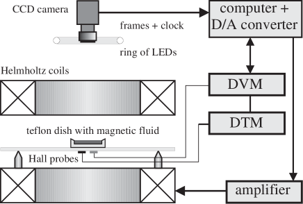
FIG. 12.: Scheme of the experimental setup

FIG. 13.: Series of snap-shots of the principal pattern evolution of the magnetic fluid for a jump from $B_{0}<B_{c}$ to $B>B_{c}$, illuminated from above by a ring of LEDs. The pictures are taken $\Delta t=180$ ms (a), $280$ ms (b), $560$ ms (c) after the start of the increase of the magnetic field.

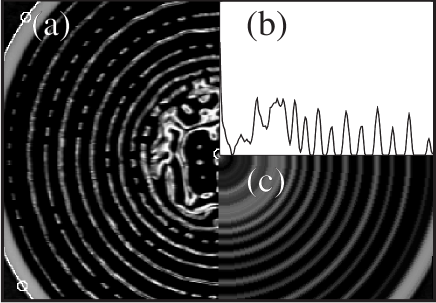
FIG. 14.: Three steps of the picture processing to extract the wave number: (a) Reflections of circular surface deformations. The white line in the left upper and lower corner marks the calculated edge of the dish, the circles on the edge serve to calculate the center of the dish. (b) Radial grey level distribution of (a). (c) Two dimensional representation of (b).

FIG. 15.: Plot of the wave number $q$ versus the magnetic induction $B$. The open squares give the experimental values, the dashed line displays the theoretical results for the material parameters of EMG 909 listed in Table I. Using $\mu_{r}$ as a fit–parameter gives the solid line.

TABLE I.: Material parameters of EMG 901 and EMG 909.

	$EMG901$	Source	$EMG909$	Source
$\mu_{r}$	$4.0$	Ferrofluidics	$1.8$	Ferrofluidics
$\rho$ [kg$\cdot$m-3]	$1.53\cdot 10^{3}$	[15]	$1.02\cdot 10^{3}$	Ferrofluidics
$\nu$ [m${}^{2}\cdot$s-1]	$6.54\cdot 10^{-6}$	Ferrofluidics	$5.88\cdot 10^{-6}$	Ferrofluidics
$\sigma$ [kg$\cdot$s-2]	$2.27\cdot 10^{-2}$	[15]	$2.65\cdot 10^{-2}$	[7]

REFERENCES

• [1] Magnetic Fluids and Application Handbook, edited by B. Berkovski and V. Bashtovoy (Begell House, New York, 1996).
• [2] M. D. Cowley and R. E. Rosensweig, J. Fluid Mech. 30, 671 (1967).
• [3] R. E. Rosensweig, Ferrohydrodynamics, (Cambridge University Press, Cambridge, 1985).
• [4] A. Gailitis, J. Fluid Mech. 82, 401 (1977).
• [5] V. G. Bashtovoi, M. S. Krakov, and A. G. Recks, Magnetohydrodynamics 21, 19 (1985)
• [6] J.-C. Bacri and D. Salin, J. Phys. (France) 45, L559 (1984).
• [7] T. Mahr, PhD thesis, Univ. Magdeburg, 1998.
• [8] We have found two references relating to constant wave numbers for a jump-like field increase. Since reference 5 in [9] is unpublished and reference 14 in [11] is an abstract not enough details are provided to assess this result.
• [9] D. Salin, Europhys. Lett. 21, 667 (1993). There is a misprint in Eq. (6) and (10).
• [10] Since $\omega$ is generally a complex number, the absolute value of $\omega$ should appear in the definition of the viscous depth, $\delta=\sqrt{2\nu/|\omega(\nu,q)|}$.
• [11] B. Abou, G. Néron de Surgy, and J. E. Wesfreid, J. Phys. II France 7 1159 (1997).
• [12] J. Weilepp and H. R. Brand, J. Phys. II France 6, 419 (1996). The constants given in Eq. (17) are correct for the magnetic boundary value problem at $z=-1$ and 00 instead of the given boundaries in Eqs. (13-14). There is a misprint in Eq. (32).
• [13] H. W. Müller, Phys. Rev. E 55, 6199 (1998).
• [14] T. Mahr and I. Rehberg, Physica D 111, 335 (1998).
• [15] Measurements conducted by A. Rothert.
• [16] A. T. Skjeltorp, J. Magn. Magn. Mat. 37, 253 (1983).
• [17] J.-C. Bacri, R. Perzynski, and D. Salin, C. R. Acad. Sci. Paris II, 307, 699 (1988).
• [18] P. A. Petit, M. P. de Albuquerque, V. Cabuil, and P. Molho, J. Magn. Magn. Mat. 113, 127 (1992).
• [19] J. Bechhoefer, V. Ego, S. Mannville, and B. Johnson, J. Fluid. Mech. 288, 325 (1995).
• [20] Hydrodynamics and Nonlinear Instabilities, edited by C. Godrèche and P. Manneville (Cambridge University Press, Cambridge, 1998), Chapt. 4.
• [21] M. C. Cross and P. C. Hohenberg, Rev. Mod. Phys., 65, 870 (1993).
• [22] J. Browaeys, J.-C. Bacri, C. Flament, S. Neveu, and R. Perzynski, Eur. Phys. J. B 9, 335 (1999).
• [23] S. Douady, J. Fluid Mech. 221, 383 (1990).
• [24] W. S. Edwards and S. Fauve, J. Fluid Mech. 278, 123 (1994).
• [25] A. G. Boudouvis, J. L. Puchalla, L. E. Scriven, and R. E. Rosensweig, J. Magn. Magn. Mat. 65, 307 (1987).
• [26] G. Néron de Surgy, J.-P. Chabrerie, and J. E. Wesfreid, IEEE T. Dielect. El. In. 2, 184 (1995).
Refer to caption