A Particle Model of Rolling Grain Ripples Under Waves

Abstract

A simple model is presented for the formation of rolling grain ripples on a flat sand bed by the oscillatory flow generated by a surface wave. An equation of motion is derived for the individual ripples, seen as “particles”, on the otherwise flat bed. The model account for the initial apperance of the ripples, the subsequent coarsening of the ripples and the final equilibrium state. The model is related to physical parameters of the problem, and an analytical approximation for the equilibrium spacing of the ripples is developed. It is found that the spacing between the ripples scale with the square-root of the non-dimensional shear stress (the Shields parameter) on a flat bed. The results of the model are compared with measurements, and reasonable agreement between the model and the measurements is demonstrated.

In the coastal zone where the water is relatively shallow, an ubiquitous phenomenon is the formation of ripples in the sand. These ripples have been described in the seminal work of Bagnold [1], who called them vortex ripples. The vortex ripples have been studied recently from a pattern forming point of view [2, 3, 4, 5]. Bagnold also described another kind of ripples which were created only from an initially flat bed, as a transient phenomena before the creation of vortex ripples. These ripples were created by the rolling back and forth of individual grains on the flat bed, and were thus called rolling grain ripples. It is this latter class of ripples which is the topic of this article.

The most well-known type of ripple created by oscillatory motion is the vortex ripple, called so because of the strong vortices created by the sharp crest of the ripples. These are the ripples one encounter when swimming along a sandy beach. The shape of the ripples is approximately triangular, with sides being at the angle of repose of the sand. The length of the ripples scale with the amplitude of the oscillatory motion of the water near bed, $a$. The dynamics of the vortex ripples and the creation of a stable equilibrium pattern has been recently described by [4].

In contrast to the vortex ripples, the rolling grain ripples are rarely (if ever) found in the field, and have only been studied in controlled laboratory experiments, where it is possible to have a completely flat bed as initial conditions. In this article the term “rolling grain ripple” refer to the ridges with triangular cross section occurring on an otherwise flat bed (Fig. 1 and Fig. 2) which is in agreement with Bagnolds definition of the rolling grain ripples (see also Plate 3 in [1]). The length of the triangular cross section is small (typically smaller than 1 cm), and much smaller than the spacing between the ridges, which again is typically smaller than the spacing between the vortex ripples. As the crest of the rolling grain ripples is rather sharp, a separation zone can be induced in the lee side of the ripple (a separation zone is an area where the flow is in the opposite direction of the main flow). This has also been found from numerical simulations of the flow over triangular ridges [6].

Bagnold assumed that there were no separation zones behind the rolling grain ripples, and this has lead to the adoption of the term rolling grain ripples for ripples without separation. It seems as if another type of ripple can emerge from a flat bed. These ripples initially have a sinusoidal shape, and thus no flat bed between them. The ripples grow and become sharper until they are steep enough to induce separation, whereafter they grow to become vortex ripples. From the authors own experience [6] and from [7], it seems as if which if these two kinds of ripples appear from a flat bed depend on the initial preparation of the bed. If the grains are small and the bed well packed, the rolling grain ripples as described by Bagnold appear (“Bagnold type rolling grain ripples”). If, however, the grains are large or the grains are carefully prepared, so as to not be packed, i.e., by letting the grains settle trough the water, a mode with sinusoidal ripples can be observed [7]. These “sinusoidal rolling grain ripples” have been described by a hydrodynamic instability of the wave boundary layer. The idea was originally formulated by Sleath [8], but was developed in great detail in a series of papers by Blondeaux, Foti and Vittori [9, 10, 11, 12, 13]. This kind of ripples is not described by the model which will be developed here.

The model to be presented is a “particle model” in the sense that it view each ripple as a “particle” which interact with its neighbouring particles. A heuristic equation of motion is written for each particle, taking into account the movement of the particle and the presence of the neighbouring particles. When two particles collide they merge and form a new, larger particle. This continues until a steady state is achieved.

After a more detailed description of the rolling grain in section I, the heuristic model is developed in section II. It turns out, fortunately, that the parameters entering this model can be connected to measurable quantities (section II A). In section II B the model is solved numerically and analytically, and comparison with experimental measurements of rolling grain ripples are done in section II C. Conclusions can be found in section IV.

I The rolling grain ripples

An example of a flat bed with rolling grain ripples coexisting with vortex ripples is seen in Fig. 1. In the middle of the picture the ripples have not yet formed and the bed is still flat, while on the top vortex ripples are seen to invade into the flat bed. The vortex ripples are typically nucleated from the boundaries or from a pertubation in the bed. In the lower part of the picture the rolling grains ripples have formed on the flat bed, and are seen as the small bands of loose grains on top of the flat bed.

The flow over the bed created by the surface wave is oscillating back and forth in a harmonic fashion. This flow creates a shear stress on the bed $\tau(t)$ which in non-dimensional form reads:

$$\theta(t)=\frac{\tau(t)}{\rho(s-1)gd}~{},$$ (1)

where $\rho$ is the density of water, $s$ is the relative density of the sand (for quartz sand in water $s=2.65$), $g$ is the gravity and $d$ is the mean diameter of the grains. $\theta$ is usually called the Shields parameter [14]. When the shear stress exceeds a critical value $\theta_{c}$, the grains start to move. For a turbulent boundary layer the value of the critical Shields parameter is $\theta_{c}\approx 0.06$ [15]. The grains which have become loosened from the bed, start to move back and forth on the flat bed, and after a while the grains come to rest in parallel bands. In the lee side of each band the bed is shielded from the full force of the flow, creating a “shadow zone” where the grains move slower than in the upstream side of the bands.

Due to this shadow zone, more grains end up in the bands than leave the bands, and they grow until they form small ridges, the rolling grain ripples. When the rolling grain ripples are fully developed, no grains will be pulled loose from the bed in the space between them, and they are stable. However, in reality the rolling grain ripples are dominated by invading vortex ripples, which is the main reason why they are rarely observed in Nature.

II A simple model

The above scenario can be formulated mathematically by writing an equation of motion for each grain/particle. In the following an equation of motion for the particles are developed. In the beginning the particles represents the grains, but as the single grains quickly merge, the particles most of the time represents a ripple. First the velocity of each particle is found, assuming that the particle is alone of the flat bed, and then the influence of the shadow zones from neighboring particles are taken into account.

Consider $N$ particles rolling on top of a rough, solid surface. Each particle is characterized by its position $x_{i}$ and its height $h_{i}$ (see Fig. 2). As the ripples are triangular, the area of each particle $A_{i}$ and their heights are related as:

$$h_{i}=\sqrt{A_{i}\tan\phi}~{},$$ (2)

where $\phi$ is the angle of repose of the sand (33^∘).

The ripple moves back and forth slower than a single grain, according to the “1/height” law. This law is well known in the study of dunes in the desert [16] or sub-aqueous dunes [17], and can be illustrated by a simple geometrical argument. Suppose there is a flux of sand over the crest of a ripple or a dune $q_{crest}$ (Fig. 3). To make the ripple move a distance $\delta x$ an amount of sand $h\delta x$ is needed. As the sediment flux is amount of sand per unit time, the velocity of the ripple is $u_{ripple}\!=\!q_{crest}/h\propto 1/h$. If the height of the initial particles (the single grains) is assumed to be equal to the grain diameter $d$, the velocity of the particles can be related to that of the single grains as:

$$u_{i}=\frac{d}{h_{i}}U_{g}\sin(\omega t)~{},$$ (3)

where $U_{g}$ is the velocity amplitude of the motion of a single grain and $\omega$ is the angular frequency of the oscillatory motion.

The flow moves back and forth and makes the particles move accordingly on top of the bed. In the wake of each particle/ripple there is a shadow zone (Fig. 4), which is the area behind the particle where the absolute value of the shear stress is smaller than it would be on a flat bed. The length of the shadow zone is therefore larger than the length of the separation bubble formed by the particle (note that the shadow zone would be present even in the absence of separation). If the shadow zone is much smaller than the amplitude of water motion, the flow in the lee side of the ripple can be assumed to have sufficient time to become fully developed. The fully developed flow over a triangle is similar to that past a backward facing step in steady flow, which has been extensively studied (see e.g. Tjerry [18]). In that case the relevant quantities, i.e., the length of the separation bubble, the length of the wake etc., scale with the height of the step. As a first assumption, the shadow zone is therefore assumed to have a length which is proportional to the height of the particle: $\alpha_{s}h_{i}$. If a particle enters the shadow zone of another particle, it is slowed down according to the distance between the particles. This means that the actual velocity of a particle is $u_{i}f(\Delta x)$ where $\Delta x$ is the distance between the grain and the nearest neighbor upstream, $u_{i}$ is the velocity of the particle outside the shadow zone and $f$ is a function determining the nature of the slowing of the motion of the particle. A simple linear function is used, as shown in Fig. 4. The exact form of the function $f$ is not crucial, as will be evident later, the important parameter being the extent of the shadow zone as determined by $\alpha_{s}$.

It is now possible to write the equations of motion for the particles as a system of coupled ODEs:

$$\dot{x_{i}}=\frac{d}{h_{i}}u_{g}(t)\underbrace{f\!\left(\frac{x_{i}-x_{i-1}}{\alpha_{s}h_{i-1}}\frac{u(t)}{|u(t)|}\right)}_{\mathrm{positive\ half\ period}}\underbrace{f\!\left(\frac{x_{i}-x_{i+1}}{\alpha_{s}h_{i+1}}\frac{u(t)}{|u(t)|}\right)}_{\mathrm{negative\ half\ period}}$$ (4)

for $i=1,\ldots,N$, where $u_{g}(t)=U_{g}\sin(\omega t)$. The motion of a particle is thus made up of three parts (i) the motion of the single undisturbed particle, (ii) the effect of the shadow from the particle to the left $(i-1)$, which might affect particle $i$ in the first half period and (iii) the effect of the shadow of the particle to the right $(i+1)$ in the second half period.

When lengths are scaled by the diameter of the grains and time by the frequency $\omega$, it is possible to identify the three relevant dimensionless parameters of the model:

  

$\alpha_{s}$, the length of the shadow zone divided by the height.

  

$a_{g}/d$, the amplitude of the motion of a single grain, divided by the grain diameter ($a_{g}=\omega U_{g}$).

  

$\lambda_{i}/d$, the initial distance between the grains; $\lambda_{i}=L/N$, where $L$ is the length of the domain and $N$ is the initial number of grains.

A Relation to physical quantities

Even though the model seem quite heuristic, the parameters entering the model, $a_{g}/d$, $\lambda_{i}/d$ and $\alpha_{s}$ can be related to physical parameters describing the flow and the properties of the grains. The line of arguments presented here closely follows those used to derive the flux of sand on a flat bed (the bed load), as can be found in text books, i.e., [15], or in [19]. First the velocity of a single grain will be derived, from which $a_{g}/d$ can be inferred. Thereafter the initial number of grains in motion is found, from which follows $\lambda_{i}/d$. Finally the length of the shadow zone $\alpha_{s}$ is discussed.

1 The velocity of the grains

The velocity of the grain can be found by considering the force balance on a single grain lying on the flat bed. The grain is subject to a drag force proportional to the square of the relative flow velocity $u_{r}=u_{nb}-u_{g}$ where $u_{nb}$ is the velocity near the bed and $u_{g}$ is the velocity of the grain:

$$F_{d}=\frac{1}{2}C_{D}\rho A|u_{r}|u_{r},$$ (5)

where $A$ is the area of the grain and $C_{D}$ is a drag coefficient. The numerical signs is used to obtain the right sign of the force. The velocity profile in the vicinity of the bed is supposed to be logarithmic. As shown in [20] this is a reasonable assumption except when the flow reverses. However, during reversal the velocities are anyway small and the accuracy is of minor importance. The logarithmic profile over a rough bed can be written as (eg. [15]):

$$u(y)=\frac{u_{f}}{\kappa}\ln\left(\frac{30y}{k_{N}}\right),$$ (6)

where $\kappa=0.41$ is the von Kármán constant, $u_{f}\equiv\sqrt{\tau/\rho}$ is the friction velocity and $k_{N}$ is the Nikuradse roughness length. It is then possible to find the near bed velocity as the velocity at $y\!\approx\!1/2d$:

$$u_{nb}=\xi u_{f}$$ (7)

where the constant $\xi$ can be determined from Eq. (6) by assuming $k_{N}=d$. Opposing the drag on the grain is the friction of the bed:

$$F_{f}=-\mu W$$ (8)

where $\mu$ is a friction coefficient and $W=\rho g(s-1)d^{3}\pi/6$ is the immersed weight of the grain. By making a balance of forces, $F_{d}+F_{f}=0$, the velocity of the grain can be found:

$$u_{g}=\xi u_{f}\left(1-\sqrt{\left|\frac{\theta_{c}}{\theta}\right|}\right),$$ (9)

where

$$\theta_{c}=\frac{4\mu}{3C_{D}\xi^{2}}~{},$$ (10)

is the critical Shields parameter. Usually $\mu=\tan\phi\approx 0.65$ [15].

2 The initial spacing of grains

Now that the velocity of the grains has been calculated, there still remains to determine the number of grains per area $n$ in motion. To this end a small volume of moving sand at the top the flat bed is considered. The balance of the forces acting on this volume is written as:

$$\tau_{b}=\tau_{G}+\tau_{c}.$$ (11)

The interpretation of the terms is as follows: The parameter $\tau_{b}$ is the shear stress on the top of the bed load layer. It is assumed that this is equal to the shear stress on a fixed flat bed. $\tau_{G}$ is the stress arising from the inter-granular collisions, giving rise to “grain-stresses” [19], modeled as: $\tau_{G}=n\mu W$. It is assumed that the inter-granular stress absorbs all the stress, except the critical stress $\tau_{c}$; this is the so-called “Bagnold hypothesis” [19]. Making Eq. (11) non-dimensional by dividing with $\rho(s-1)gd$, the number of grains in motion is found as:

$$n=\frac{6}{\pi d^{2}\mu}(\theta-\theta_{c}),$$ (12)

If $\theta<\theta_{c}$, then no grains are in motion and $n=0$. $n$ can also be viewed as the initial density of grains, and by assuming a square packing of the grains the initial distance between the grains becomes:

$$\frac{\lambda_{i}}{d} = \frac{1}{\sqrt{n}d}$$ (13)

$$= \sqrt{\frac{\pi\mu}{6(\theta-\theta_{c})}}.$$ (14)

3 The length of the shadow zone

The last parameter $\alpha_{s}$, which characterize the length of the shadow zone, is a bit harder to estimate accurately. By exploring the analogy with the backward facing step which was suggested in section II, we can get some bounds for $\alpha_{s}$. In the backward facing step there is a zone with flow separation which extends approximately 6 step heights from the step, see Fig. 5. After approximately 16 step heights there is a point where the shear stress has a small maximum. It follow that the length of the shadow zone should be longer than the separation zone, but shorter that the point of the maximum in the shear stress, i.e., $6<\alpha_{s}<16$.

B Numerical and analytical solutions of the model

In the following section the behavior of the model is examined. To study the detailed behavior the set of coupled ordinary differential equations (4) is integrated numerically. It is seen that the model reaches a steady state and an analytical expression for the spacing between the ripples in the steady state is developed.

The numerical simulations in this section are based on a simple example with $a_{g}/d\!=\!35$ and $\lambda_{i}/d\!=\!3.23$ and $\alpha_{s}$ is set to 10. As initial condition all particles have an area of $1.0\ \pm$ 10 %, to add some perturbation. The initial number of particles $N$ in this example is 800.

In the first few periods a lot of grains is colliding and merging (Fig. 6). As the ripples are formed and grow bigger the evolution slows down, until a steady state is reached (Fig. 7). The spacing between the ripples in the steady state show some scatter around the average value, which is also observed in experiments. The variation in the average spacing of the steady state $\lambda_{eq}$ for realizations with different initial random seed, turned out to be on the order of $1/N_{eq}$ where $N_{eq}$ is the final number of ripples.

To study the behavior of the average spacing of the ripples $\lambda_{eq}$, a number of simulations were made where the parameters were varied one at a time. Each run was started from the initial disordered state.

Changing $a_{g}/d$ only results in a minor change in the spacing of the ripples (Fig. 8a). The final spacing between the ripples does depend on the length of the shadow zone $\alpha_{s}$; the longer the shadow zone, the longer the ripples (Fig. 8b). This can be used to estimate the average equilibrium spacing between the ripples. When the distance between two ripples is longer than the shadow zone of the ripples, they are no longer able to interact. This gives:

$$\lambda_{eq}>\alpha_{s}h_{eq},$$ (15)

where subscript $eq$ denotes average value at equilibrium. However if two ripples have a spacing just barely shorter than Eq. (15), they will be able to interact and eventually they will merge. One can therefore expect to find spacings up to $\lambda_{eq}\!<\!2\alpha_{s}h_{eq}$. Assuming that the average length is in between the two bounds one get:

$$\lambda_{eq}=\gamma\alpha_{s}h_{eq},\quad 1<\gamma<2~{}.$$ (16)

where $\gamma$ can be found by comparing the results from the full simulations with Eq. (16). The height of the ripples at equilibrium can be found by splitting the initial number of particles evenly onto the equilibrium ripples. Then the average area at equilibrium is $A_{eq}\!=\!\lambda_{eq}/\lambda_{i}d^{2}$ and from Eq. (2) follows that the height is $h_{eq}/d\!=\!\sqrt{\tan\phi\,\lambda_{eq}/\lambda_{i}}$, which gives an average equilibrium spacing:

$$\frac{\lambda_{eq}}{d} = \gamma^{2}\frac{\alpha_{s}^{2}d\tan\phi}{\lambda_{i}}$$ (17)

$$= \alpha_{s}^{2}\gamma^{2}\sqrt{\frac{6\tan\phi}{\pi}}\sqrt{\theta-\theta_{c}}~{}.$$ (18)

The equilibrium spacing is therefore found to be proportional to $\sqrt{\theta\!-\!\theta_{c}}$ with the constant of proportionality being made up of $\alpha_{s}$, $\gamma$ and various geometrical factors. All the quantities related to the dynamical evolution of the ripples, i.e., the velocity of the ripples, the shape of the function $f(\Delta x)$ etc. does not enter into the expression.

C Comparison with experiments

The only parameter that has not been accurately determined is $\alpha_{s}$. The value of this parameter can be estimated by comparison with measurements.

In 1976, Sleath made a series of experiments, measuring spacing between rolling grain ripples [8]. The ripples were formed on a flat tray oscillating in still water using sand of two different grain sizes: 0.4 mm and 1.14 mm. To compare with the experiments the value of $\theta$ need to be calculated. $\theta$ reflect the number of grains in motion, and it seems natural to use the maximum value during the wave period, $\theta_{max}$. To estimate $\theta_{max}$ the shear stress on the bed has to be estimated. The maximum shear stress on the bed, $\tau_{max}$ during a wave period can be found using the concept of a constant friction factor $f_{w}$ ([21]):

$$\tau_{max}=\frac{1}{2}\rho f_{w}u_{max}^{2},$$ (19)

with $u_{max}$ being the maximum near-bed velocity. The friction factor can be estimated using the empirical relation [15]:

$$f_{w}=0.04\left(\frac{a}{k_{N}}\right)^{-0.25}$$ (20)

where $a=u_{max}\omega$ and $k_{N}\simeq d$.

The range of Shields parameters in the experiments was found in this way to range from the critical Shields parameter to $\theta=0.42$. For the high Shields parameters the rolling grain ripples were reported to be very unstable, and to quickly develop into vortex ripples. In these cases, the measured ripple spacing then reflects the spacing between the rolling grain ripples before they developed into vortex ripples [8].

In Fig. 9 the experimental results are compared with runs of the model using $\alpha_{s}=15.0$ (the reason for this particular value will be clear shortly) and $N=10000$. By fitting all the runs to Eq. (16) it was found that $\gamma=1.40$. The results using Eq. (18) and $\gamma=1.40$ are shown with a line.

First of all, it is seen that Eq. (18) predicts the results from the full model Eq.(4) well. The correspondence between the model and the experiments is reasonable, but there are some systematic discrepancies, which will be discussed.

There are some few points with small ripple spacing for which the model does not fit the measurements. These measurements has a Shields parameter very near the critical (i.e., just around the onset of grain motion), which implies some additional complications. The grains used in the experiment were not of a uniform size; rather they were part of a distribution of grain sizes, and the grain size reported is then the median of the distribution, $d_{50}$. The Shields parameter is calculated using the median of the distribution, but actually one could calculate a Shields parameter for different fractions of the distribution, thus creating a $\theta_{10}$, a $\theta_{50}$ etc.. When $\theta_{50}$ is smaller than then the critical Shields parameter, $\theta_{10}$ might still be higher than the critical Shields parameter. This implies that grains with a diameter smaller than $d_{50}$ will be in motion, while the larger grains will stay in the bed. As only $d_{50}$ is used in the calculation of the equilibrium ripple spacing, the distance between the grains $\lambda_{i}$ will be overestimated near the critical Shields parameter, where the effect of the poly-dispersity is expected to be strongest. An overestimation of $\lambda_{i}$ will lead to an under-prediction of the ripple length, which is exactly what is seen in Fig. 9.

There are also three points from the experiments taken at very large Shields parameters, which seems to be a bit outside the prediction of the model. As already mentioned, these points are probably doubtful because of the very fast growth of vortex ripples. It is therefore reasonable to assume that vortex ripples invaded the rolling grain ripples before these had time to reach their full length.

To find a reasonable value of $\alpha_{s}$ Eq. (18) was fitted to the experimental points. To avoid the points which might be of doubtful quality, as discussed above, only the points in the range $0.075\!<\!\theta\!<\!0.3$ were used. This gave the value of $\alpha_{s}\!=\!15.0$, in agreement with the qualitative arguments in section II A 3.

III Discussion of the results

From the comparison of the model with measurements it seems as if the model confidently reproduces the experiments.

In the model the number of grains in motion is constant (even though the number of particles changes). In an experimental situation, however, new grains might be lifted from the bed and added to the initial number of grains in motion. As the part of the flat bed between the ripples is covered by the shadow zones of the particles, these stretches will be shielded from the full force of the flow, and only very slowly will new grains be loosened here. This small addition of new grains will result in a slow growth of the rolling grain ripples, such that eventually grow into vortex ripples. This slow growth is very well illustrated by recent measurements [2], but not covered by the present model.

IV Conclusion

In conclusion, a model has been created which explain the creation and the equilibrium state of rolling grain ripples of the type described by Bagnold. The final distance between the ripples is proportional to $\sqrt{\theta-\theta_{c}}$. The model has been compared with measurements with reasonable agreement.

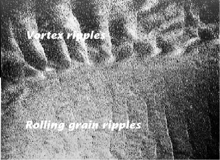
FIG. 1.: An example of a flat bed viewed from above, with rolling grain ripples (bottom) and vortex ripples invading from the top. The experimental setup is a wave tank 60 cm wide and approximately 50 cm deep, containing sand with a median diameter of $0.2$ mm.

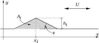
FIG. 2.: A sketch of a ripple on the flat bed with related quantities.

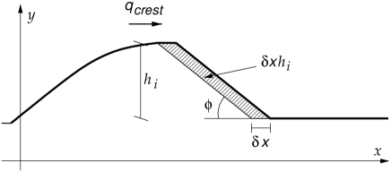
FIG. 3.: Geometrical illustration of the quantities involved in the derivation of the one-over-h law.

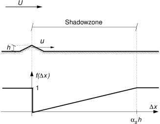
FIG. 4.: An illustration of the shadow zone of one ripple, in the part of the wave period where the flow is from the left to the right. Below is seen the function $f(\Delta x)$ used to describe how a particle is slowed down when it enters the shadow zone of another particle.

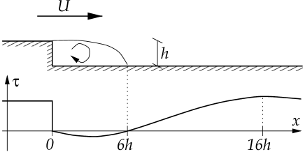
FIG. 5.: A sketch of the shear stress on the bed during a steady flow over a backward facing step.

FIG. 6.: Zoom of the movement of the particle in the first two wave periods. $a_{g}/d=35$, $\lambda_{f}=3.23$ and $\alpha_{s}=10.0$.

FIG. 7.: The development of the particles until steady state is reached. The lines show the positions of the particles at the end of each period.

FIG. 8.: The spacing between the rolling grain ripples at equilibrium as a function of the initial density of grains. The basic example is shown with the circles: $a_{g}/d=35$ and $\alpha_{s}=10.0$. In a) the value of $a_{g}/d$ is varied, for pluses $a_{g}/d=20$, crosses $a_{g}/d=50$. In b) $\alpha_{s}$ is varied; pluses: $\alpha_{s}=7$, crosses: $\alpha_{s}=13$.

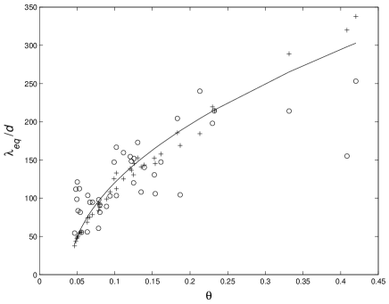
FIG. 9.: Comparison between the measured wave lengths of rolling grain ripples (circles), with results from the model (pluses), and from Eq. (16) with $\gamma\!=\!1.40$ (the line). The value of $\alpha_{s}$ is $15.0$. The critical Shields parameter is 0.04 and $\mu\!=\!0.65$.

- [1] R. A. Bagnold. Motion of waves in shallow water, interaction between waves and sand bottoms. Proc. Roy. Soc. of London, A187:1–15, 1946.
- [2] A. Stegner and J.E. Wesfreid. Dynamical evolution of sand ripples under water. Phys. Rev. E, 60(4), 1999.
- [3] M. A. Scherer, F. Melo, and M. Marder. Sand ripples in an oscillating annular sand-water cell. Physics of Fluids, 11(1):58–67, 1999.
- [4] K.H. Andersen, M.-L. Chabanol, and M.v. Hecke. Dynamical models for sand ripples beneath surface waves. In preparation, 2000.
- [5] A. Haaning, C. Ellegaard, M.v. Hecke, J. Lundbek, and T. Sams. In preparation, 2000.
- [6] K.H. Andersen. Ripples Beneath Surface Waves and Topics in Shell Models of Turbulence. PhD thesis, the Niels Bohr Institute, Copenhagen University, http://www.isva.dtu.dk/ken/Thesis.html, 1999.
- [7] E. Foti. Pers.comm.
- [8] J.F.A. Sleath. On rolling-grain ripples. Journal of Hydraulic Research, 14(1):69–81, 1976.
- [9] P. Blondeaux. Sand ripples under sea-waves. part 1. ripple formation. Journal of Fluid Mechanics, 218:1–17, 1990.
- [10] G. Vittori and P. Blondeaux. Sand ripples under sea waves. part 2. finite-amplitude development. Journal of Fluid Mechanics, 218:19–39, 1990.
- [11] G. Vittori and P. Blondeaux. Sand ripples under sea waves. part 3: Brick-pattern ripple formation. Journal of Fluid Mechanics, 239:23–45, 1991.
- [12] E. Foti and P. Blondeux. Sea ripple formation: The turbulent boundary layer case. Coastal Engineering, 25:227–236, 1995.
- [13] E. Foti and P. Blondeux. Sea ripple formation: The heterogeneous sediment case. Coastal Engineering, 25:237–253, 1995.
- [14] I.A. Shields. Anwendung der Aehnlichkeitsmechanik under der Turbulenzforshung auf die Geschiebebbewegung. Mitt. Preuss. Versuchanstalt, Berlin, 26, 1936.
- [15] J. Fredsøe and R. Deigaard. Mechanics of Coastal Sediment Transport. World Scientific, 1992.
- [16] H. Nishimori, M. Yamasaki, and K.H. Andersen. A simple model for the various pattern dynamics of dunes. International journal of modern physics B, 12(3):257–272, 1998.
- [17] J. Fredsøe. The stability of a sandy river bed. In T. Nakato and R. Ettema, editors, Issues and directions in hydraulics, pages 99–113. Iowa Institute of Hydraulic Research, 1996.
- [18] S. Tjerry. Morphological calculation of dunes in alluvial rivers. PhD thesis, ISVA, the Danish Technical University, 1995.
- [19] A. Kovacs and G. Parker. A new vectorial bedload formulation and its application to the time evolution of straight river channels. Journal of Fluid Mechanics, 267:153–183, 1994.
- [20] B.L. Jensen, B.M. Sumer and J. Fredsøe. Turbulent oscillatory boundary layers at high Reynolds numbers. Journal of Fluid Mechanics, (206)265–297 (1989).
- [21] I.G. Jonsson and N.A. Carlsen. Experimental and theoretical investigations in an oscillatory turbulent boundary layer. Journal of Hydraulic Research, 14(1):45–60, 1976.