Approximate solutions and scaling transformations for quadratic solitons

Abstract

We study quadratic solitons supported by two- and three-wave parametric interactions in $\chi^{(2)}$ nonlinear media. Both planar and two-dimensional cases are considered. We obtain very accurate, ’almost exact’, explicit analytical solutions, matching the actual bright soliton profiles, with the help of a specially-developed approach, based on analysis of the scaling properties. Additionally, we use these approximations to describe the linear tails of solitary waves which are related to the properties of the soliton bound states.

I Introduction

One of the rapidly expanding areas of research is the physics of solitons – wave packets, or self-trapped beams, that propagate with their profiles remaining undistorted. In particular, parametric solitons, composed of mutually trapped fundamental and harmonic waves, attract interest of researchers due to a wide range of possible applications. In optics, for example, such solitons were observed in media with quadratic (or $\chi^{(2)}$) nonlinearity, and their unique features can be utilized for the creation of all-optical information processing devices [1]. In general, parametric solitons may form in different media which possess resonant quadratic nonlinearities, such as plasma, organic superlattices [2], Bose-Einstein condensate [3], etc.

Many papers have been devoted to a theoretical analysis of quadratic solitons [4]. It was shown that bright solitons can be stable, and hence are of most interest for practical applications, on the other hand parametric dark solitons often exhibit modulation instability. However, due to nontrivial features of the resonant coupling, there still remain some properties of the bright quadratic solitons which have not been thoroughly described or completely understood. The problem here is that the governing equations are not integrable, and general analytical solutions can’t be constructed. Thus, the variational method [5] was widely used to find approximate solutions. In this approach, the free parameters controlling the trial functions are found by minimizing the Lagrangian functional. A rarely mentioned limitation here is that this technique imposes very strong restrictions on the class of the trial functions, for the parameters to be found in an explicit form. This becomes a real drawback if these test functions are not quite suitable for the problem at hand (see, e.g., Ref [6]).

In this paper we introduce a different approach for obtaining approximate expressions for the soliton envelopes. At first we choose trial functions which can precisely describe the actual soliton profiles. This step involves the analysis of the scaling properties of a soliton family, i.e. how the envelopes are transformed as a free parameter (propagation constant) is altered. Secondly, a specially developed technique is used to find the fitting parameters. It will be demonstrated that the resulting solutions turn out to be extremely accurate.

The rest of the paper is organized as following. First, two-wave solitons in planar structures are studied. Then, the analysis is extended to the case of three wave mutual trapping in an anisotropic medium. Finally, the properties of two-component solitary beams propagating in a bulk medium are investigated.

II One dimensional solitons

A Two-wave solitons

1 Basic equations and their properties

Parametric interaction between the fundamental frequency (FF) wave and its second harmonic (SH) in the (1+1) dimensional case can be described by a set of coupled equations for slowly varying complex amplitudes of the wave packets [7] (see also [4, 8]). We consider the case when there is no walk-off, and then in normalized variables have [9]:

$$\begin{array}[]{l}{\displaystyle i\frac{\partial u}{\partial z}+\frac{\partial^{2}u}{\partial x^{2}}+u^{*}w=0,}\\[9.0pt] {\displaystyle i\sigma\frac{\partial w}{\partial z}+\frac{\partial^{2}w}{\partial x^{2}}-\beta w+\frac{1}{2}u^{2}=0,}\end{array}$$ (1)

where $u(x,z)$ and $w(x,z)$ are the FF and SH amplitudes correspondingly, $z$ is the propagation distance, and the parameter $\beta$ characterizes the mismatch of the linear phase velocities. These equations can describe: (i) spatial beams in a slab waveguide, exhibiting diffraction in the transverse direction $x$, where $\sigma\approx 2$; or (ii) temporal pulses, where $x$ stands for the retarded time and $\sigma>0$ is the ratio of the absolute values of second-order dispersion coefficients (the signs are those which allow stable bright solutions).

Under certain conditions, mutual trapping of two waves can be achieved, when diffraction (or second-order dispersion) is exactly compensated for by nonlinear refraction. Such stationary propagation is observed for a special class of beams (or temporal wave packets) – solitons. To find their profiles, we look for solutions of Eqs. (1) in the form

$$\begin{array}[]{l}{\displaystyle u(x,z)=\lambda u_{0}\left(x\sqrt{\lambda}\right)e^{i\lambda z},}\\[9.0pt] {\displaystyle w(x,z)=\lambda w_{0}\left(x\sqrt{\lambda}\right)e^{2i\lambda z},}\end{array}$$ (2)

where $u_{0}$ and $w_{0}$ are the real envelope amplitudes, and $\lambda>0$ is the propagation constant. After substituting expressions (2) into Eqs. (1), the following system of coupled ordinary differential equations can be derived:

$$\begin{array}[]{l}{\displaystyle\frac{d^{2}u_{0}}{dx^{2}}-u_{0}+u_{0}w_{0}=0,}\\[9.0pt] {\displaystyle\frac{d^{2}w_{0}}{dx^{2}}-\alpha w_{0}+\frac{1}{2}u_{0}^{2}=0,}\end{array}$$ (3)

where the only free parameter is the normalized mismatch $\alpha=2\sigma+\beta/\lambda$.

For localized waves, described by Eqs. (1), the total power $P$ and Hamiltonian $H$ are conserved [7]. The values of these integral characteristics, corresponding to solitons defined by Eqs. (3), can be found as [10]:

$$P=\lambda^{3/2}P_{0},\,H=\lambda^{5/2}(H_{0}-P_{0}).$$ (4)

Here the renormalized power and Hamiltonian are $P_{0}=P_{u_{0}}+2\sigma P_{w_{0}}$ and $H_{0}=0.4(P_{u_{0}}+\alpha P_{w_{0}})$, where

$$P_{u_{0}}=\int_{-\infty}^{+\infty}u_{0}^{2}dx,\,P_{w_{0}}=\int_{-\infty}^{+\infty}w_{0}^{2}dx,$$ (5)

We are looking for bright solitons, where the field decays at infinity. Such solutions of Eqs. (3) were found numerically for any $\alpha>0$ [9, 11, 12] and corresponding solitons were shown to be stable for mismatches $\alpha>\alpha_{\rm cr}$ [13]. Here, the critical parameter value $\alpha_{\rm cr}$ is a function of $\sigma$, and for spatial solitons ${\left.\alpha_{\rm cr}\right|}_{\sigma=2}\approx 0.2$.

The properties of this soliton family were extensively studied in the literature. An exact solution was found at $\alpha=1$ [7]:

$$w_{0}(x)=u_{0}(x)/\sqrt{2}={\left(3/2\right)}\;{\rm sech}^{2}\left(x/2\right).$$ (6)

On the other hand, for large mismatches, $\alpha\rightarrow\infty$, the SH component approaches $w_{0}(x)\simeq v_{0}^{2}(x)/{\left(2\alpha\right)}$. Then, in this so-called cascading limit, the FF wave is determined as a solution of the nonlinear Schrödinger equation (NLSE), and the wave envelopes are [8, 14]:

$$v_{0}(x)\simeq 2\sqrt{\alpha}\;{\rm sech}(x),\;w_{0}(x)\simeq 2\;{\rm sech}^{2}(x).$$ (7)

This solution can be improved by taking into account higher-order terms in a series decomposition over a small parameter, $\alpha^{-1}$ [15, 16]. However, this approach leads to cumbersome expressions which are somewhat hard to analyze.

Exact analytical solutions of Eqs. (3) cannot be found for arbitrary values of $\alpha$. Thus, in order to obtain approximate solutions for the soliton profiles, the variational approach was used. Calculations with an ansatz in the form of Gaussian functions predict the power distribution between the FF and SH components quite accurately, and provide a close estimation for the maximum amplitudes in the whole parameter range $0<\alpha<\infty$ [16, 17]. However, the trial functions do not correspond to the actual wave profiles, and thus the ”tails”, or amplitude asymptotics at $x\rightarrow\pm\infty$, are not described well. In other studies [18], the profiles of the trial functions are chosen as scaled exact solutions (6) or (7) with arbitrary amplitudes, but fixed relative widths for the FF and SH wave packets. Due to this limitation, precise results are obtained only for $\alpha\approx 1$ and $\alpha\rightarrow\infty$ respectively.

2 Approximate analytical solution

In order to construct a solution without the above mentioned drawbacks, we want to take into account some characteristic properties of the bright solitons. Specifically, we notice that the form of the SH envelope is the same at $\alpha=1$ and $\alpha\rightarrow\infty$ [see Eqs. (6) and (7)]. Moreover, we perform numerical simulations and observe a very remarkable fact: for $\alpha\geq 1$, $w_{0}(x)$ remains almost self similar. Thus, we search for an approximate solution with the SH component in the form:

$$w_{0}(x)=w_{m}{\rm sech}^{2}{\left(x/p\right)},$$ (8)

where the maximum amplitude $w_{m}$ and characteristic width $p$ are unknown parameters. Then, the FF component profile can be determined using the first equation in (3). This is a linear eigenvalue problem, which has an exact solution for the effective waveguide created by the SH field (8). In a single bright soliton, $u_{0}(x)$ doesn’t have zeros, and thus we take the fundamental mode. This requirement leads to a relation between the parameters of an effective waveguide:

$$w_{m}=1+1/p.$$ (9)

Then the corresponding FF profile is found to be

$$u_{0}(x)=u_{m}{\rm sech}^{p}{\left(x/p\right)},$$ (10)

where $u_{m}$ is the peak amplitude.

Our trial functions do not satisfy the SH equation in (3) exactly, and thus it should be matched approximately. This can be done with the help of the variational method. However, this leads to a set of transcendental equations, and then the solution parameters can’t be expressed in an explicit form. As our aim is to derive a simple analytical approximation, which should be easy to analyze and use in calculations, we choose another approach. First, in order to match the soliton peak, we require the equation for the SH amplitude in (3) to be exactly satisfied at the soliton center, $x=0$, and thus obtain:

$$2w_{m}{\left(\alpha+2/p^{2}\right)}=u_{m}^{2}.$$ (11)

Secondly, we notice that Eqs. (3) describe an equivalent dynamical problem, viz. particle movement with generalized velocities $\left(du_{0}/dx,dw_{0}/dx\right)$ in a potential $U_{d}(u_{0},w_{0})={\left(u_{0}^{2}w_{0}-u_{0}^{2}-\alpha w_{0}^{2}\right)}/2$. This is a conservative system, with Hamiltonian $H_{d}={{\left(du_{0}/dx\right)}^{2}}/2+{{\left(dw_{0}/dx\right)}^{2}}/2+U_{d}(u_{0},w_{0})$. For bright solitons, the field vanishes at infinity, and thus $H_{d}\equiv 0$. Then, as the functions $u_{0}(x)$ and $w_{0}(x)$ reach their maximum values at $x=0$, the corresponding derivatives are zero, and thus the necessary condition for a zero asymptotic is $\left.H_{d}\right|_{x=0}=\left.U_{d}\right|_{x=0}=0$, which we use to relate the peak amplitudes:

$$u_{m}^{2}w_{m}-u_{m}^{2}-\alpha w_{m}^{2}=0.$$ (12)

Combining Eqs. (8)-(12), we obtain an approximate solution in the following simple form:

$$\begin{array}[]{l}{\displaystyle u_{0}(x)={u_{m}}{{\rm sech}^{p}(x/p)},\;\;\;w_{0}(x)={w_{m}}{{\rm sech}^{2}(x/p)},}\\[9.0pt] {\displaystyle u_{m}^{2}=\frac{\alpha w_{m}^{2}}{\left(w_{m}-1\right)},\;p=\frac{1}{\left(w_{m}-1\right)},\;\alpha=\frac{4{\left(w_{m}-1\right)}^{3}}{\left(2-w_{m}\right)}.}\end{array}$$ (13)

Here, the last relation allows us to determine $w_{m}$ for an arbitrary $\alpha$ as a solution of a cubic equation, and then to find all other parameters as functions of $\alpha$. For mismatches in the interval $0<\alpha<+\infty$, the parameter values change monotonically in the ranges: $0<u_{m}<+\infty$, $1<w_{m}<2$, and $+\infty>p>1$. At $\alpha=1$ the values are $u_{m}=3/\sqrt{2}$, $w_{m}=3/2$, $p=2$, i.e. our general expression reduces to the exact solution (6). Similarly, for $\alpha\rightarrow+\infty$ the limiting result (7) follows.

3 Soliton tails

As one of our goals is to describe the soliton tails, let us have a look at the far-field asymptotics that follow from Eqs. (13). It is easy to check that the FF profile exactly matches the linear limit. To understand the properties of the SH component tails, we notice that the corresponding equation in Eqs. (3) describes the motion of a particle driven by an external force $u_{0}^{2}/2$. As this expression is positive, the function $w_{0}(x)$ can’t decay faster than that in the linear limit: $w_{0}(x)\sim\exp{\left(-\sqrt{\alpha}|x|\right)}$. Indeed, for $\alpha>1$, we have $p<2$, i.e. the FF component is effectively wider than the SH, and thus the field decay rate is smaller, as is correctly predicted by Eqs. (13). In contrast, for $\alpha<1$ the width of the FF component is smaller than that of the SH (as $p<2$), and then the SH tails are to be determined by linear asymptotics. However, the solution (13) overestimates the SH field localization. To account for this feature, we sue the soliton ‘peak’ from (13) with a linear tail, so that the function and its first derivative change continuously, and obtain a more accurate expression for the SH component in the case $\alpha<1$:

$$w_{0}(x)=\left\{\begin{array}[]{l}{\displaystyle w_{m}{\rm sech}^{2}\left(x/p\right),\,{\left|x\right|}\leq x_{a},}\\[9.0pt] {\displaystyle w_{0}(x_{a})\exp{\left[-\sqrt{\alpha}{\left({\left|x\right|}-x_{a}\right)}\right]},\,{\left|x\right|}>x_{a},}\end{array}\right.$$ (14)

where $x_{a}={\left(p/2\right)}\ln{\left[\left(2+p\sqrt{\alpha}\right)/\left(2-p\sqrt{\alpha}\right)\right]}$. From Eq. (14) it follows that the SH profile becomes double scaled. That is, we predict the existence of linear tails in the SH component, which are effectively not trapped by the FF field, and carry some power:

$$P_{a}=2\int_{x_{a}}^{+\infty}w_{0}^{2}dx=[w_{0}(x_{a})]^{2}/\sqrt{\alpha}.$$ (15)

The dependence of the linear tail parameters on the normalized mismatch $\alpha$ is shown in Fig. 1.

FIG. 1.: Dependence of the SH linear tails characteristics on mismatch $\alpha$: (a) separation from the soliton center $x_{a}$ and (b) associated normalized power $P_{a}$.

4 Soliton bound states

A connection between the soliton bound states and the linear tails has been demonstrated for many physical situations. For example, mutual trapping of radiating parametric bright solitons was shown to be possible for a discrete set of propagation constant values when, due to destructive interference, the oscillatory tails disappear [19]. However, in our case the localized modes are not in resonance with propagating linear waves [9], and a natural assumption is that the solitons can trap each other by their linear tails for a continuous range of mismatches. This physical picture is consistent with the results of the previous numerical simulations and analytical investigations, showing that multi-soliton states are possible only for $\alpha<1$ [12, 17, 20, 21]. Moreover, the characteristic distance between the neighboring solitons can be roughly estimated to be of order $2x_{a}$, and this expression predicts the non-monotonic dependence of the separation on mismatch $\alpha$. The minimum separation should be observed for the mismatch corresponding to an extremum point, $\left.dx_{a}/d\alpha\right|_{\alpha_{\rm ma}}=0$, and then it follows that $\alpha_{\rm ma}\simeq 0.12$, see Fig. 1(a). Quite remarkably, this mismatch value corresponds very closely to the results of numerical calculations, see Fig. 4 in Ref. [21].

FIG. 2.: Left: Comparison between numerical results (continuous curves) and approximate analytical solutions (crosses) given by Eqs. (13)-(14). The characteristics are: (a,b) maximum amplitudes of the FF and SH, (c) total power (for the case $\sigma=2$), and (d) Hamiltonian.
Right: Corresponding relative errors are shown with solid lines, and dotted lines present deviations for the SGP.

5 Comparison with numerical results

In order to determine deviations between the approximate and exact solutions, we solved Eqs. (3) numerically. The corresponding dependencies of the peak amplitudes, total power, and Hamiltonian on the detuning parameter $\alpha$ are presented in Fig. 2 (left graphs) for the case of spatial solitons ($\sigma=2$). As a matter of fact, the numerical and analytical results on these plots are not distinguishable, and that is why we show them differently, by continuous curves and asterisks. Plots on the right give corresponding relative deviations with solid lines, and dashed lines demonstrate the errors for the variational solution with Gaussian profiles (SGP) [16, 17]. We see that the analytical solution (13)-(14) describes the key soliton parameters extremely accurately. In a wide region of mismatch values, $\alpha>1$, the relative errors are smaller than 0.7% for the total power, and 0.3% for other characteristics. For $\alpha<1$ the deviations become larger, but do not exceed 3%. It is clear that our solution gives much more accurate results than the SGP, and the latter provides a slightly better estimation for the total power only in a narrow region of mismatches.

At this point we would like to stress that the above-mentioned characteristics are not the only ones which determine the ‘quality’ of the approximate solutions. The closeness of the approximate component profiles to exact soliton envelopes, including the tails, is also very important. From Figs. 3(a) and 3(b), we see that the solution (13)-(14) describes the profiles very accurately as well (left plots), unlike the SGP which matches them only ‘on average’ (see plots on the right). To characterize the accuracy numerically, we define the relative deviations as:

$$\begin{array}[]{l}{\displaystyle\delta_{u}=\ln{\frac{\int_{-\infty}^{+\infty}{\left|u_{0}^{\rm exact}-u_{0}^{\rm approx.}\right|}^{2}dx}{\int_{-\infty}^{+\infty}{\left|u_{0}^{\rm exact}\right|}^{2}dx}},}\\[15.0pt] {\displaystyle\delta_{w}=\ln{\frac{\int_{-\infty}^{+\infty}{\left|w_{0}^{\rm exact}-w_{0}^{\rm approx.}\right|}^{2}dx}{\int_{-\infty}^{+\infty}{\left|w_{0}^{\rm exact}\right|}^{2}dx}}.}\end{array}$$ (16)

Note that these characteristics have a dB-like scale, i.e. smaller negative values mean better matching. In Fig. 3(c), the errors corresponding to solution (13)-(14) are shown on the left, and to SGP on the right. We see that our approach allows us to precisely describe the soliton profiles, both peaks and tails, for any mismatch $\alpha$. That is why we were able to reveal some remarkable features of two-component parametric mutual trapping for $\alpha<1$, when the SH field configuration becomes double scaled [see Eq. (14),(15) and relating discussions]. On the other hand, the SGP does not provide close estimations for the actual profiles, especially for $\alpha<1$, where the discrepancies increase drastically.

Approximate solutions can be used not only in theoretical studies, but also in numerical simulations. The unique accuracy of solution (13)-(14) makes it an almost perfect generator for ‘soliton’ input conditions. We checked that the initial propagation stage is accompanied by very minor oscillations, and that the associated power loss due to radiation is negligible [see, e.g., Fig. 4].

FIG. 3.: Comparison of numerical results with analytical predictions: solution (13)-(14), on the left, and the SGP, on the right. Dotted lines correspond to the FF and solid lines to the SH components. (a,b) Two-wave soliton profiles at $\alpha=4$ and $\alpha=0.01$ respectively. Continuous curves show exact numerical and crosses show approximate solutions. (c) Deviations of approximate profiles as defined in Eqs. (16).

To summarize, the approximate analytical solution, given in a compact explicit form by Eqs. (13)-(14), describes virtually all principal features of the soliton family. That is why it can be called ‘almost exact’. We might wonder, why is it so accurate? The key point in the analysis was to take into account the self-similarity of the SH envelopes. Then, we can view Eqs. (13)-(14) as approximate scaling transformations of the two-wave bright soliton family.

FIG. 4.: Almost stationary evolution of the FF (a) and SH (b). The initial condition is given by the approximate two-wave soliton solution (13) at $\alpha=4$, $\sigma=2$, $\lambda=1$.

B Three-wave interaction in anisotropic medium

Let us now investigate a more general case of three-wave interaction. Following Ref. [22], we consider a double-phase matched wave interaction, such that the FF waves of fundamental orthogonal polarizations (i.e. ordinary and extraordinary) are coupled with the same SH component. That is, the full FF field is now vectorial, $\overrightarrow{U}=\{u,v\}$, and the two components are determined as

$$\begin{array}[]{l}{\displaystyle u(x,z)=U(x,z)\cos\left[\varphi(x,z)\right],}\\[9.0pt] {\displaystyle v(x,z)=U(x,z)\sin\left[\varphi(x,z)\right],}\end{array}$$ (17)

where $\varphi(x,z)$ is the polarization angle. For such a configuration the system of normalized equations can be written in the following form [22]:

$$\begin{array}[]{l}{\displaystyle i\frac{\partial u}{\partial z}+\frac{\partial^{2}u}{\partial x^{2}}+u^{\ast}w=0,}\\[9.0pt] {\displaystyle i\frac{\partial v}{\partial z}+\frac{\partial^{2}v}{\partial x^{2}}-\beta_{1}v+\chi v^{\ast}w=0,}\\[9.0pt] {\displaystyle i\sigma\frac{\partial w}{\partial z}+\frac{\partial^{2}w}{\partial x^{2}}-\beta w+\frac{1}{2}(u^{2}+v^{2})=0.}\end{array}$$ (18)

Here $\chi$ is the normalized component of the $\chi^{(2)}$ nonlinear susceptibility matrix, characterizing the $v\leftrightarrow w$ coupling ‘strength’ in relation to the $u\leftrightarrow w$ parametric interaction process, and $\beta_{1}$ is the phase mismatch between the orthogonally-polarized FF components. All the other parameters have the same meaning as in Eqs. (1).

We are interested in bright solitons supported by Eqs. (18), and search for solutions in the form:

$$\begin{array}[]{l}{\displaystyle u(x,z)=\lambda u_{0}(x\sqrt{\lambda})e^{i\lambda z},}\\[9.0pt] {\displaystyle v(x,z)=\lambda v_{0}(x\sqrt{\lambda})e^{i\lambda z},}\\[9.0pt] {\displaystyle w(x,z)=\lambda w_{0}(x\sqrt{\lambda})e^{2i\lambda z},}\end{array}$$ (19)

where $u_{0}$ and $v_{0}$ are the real stationary amplitudes of the FF waves with orthogonal polarizations, $w_{0}$ is the envelope of the SH component, and $\lambda>0$ is the propagation constant. Then, we substitute Eqs. (19) into the original system (18) and find a set of coupled equations for the soliton profiles:

$$\begin{array}[]{l}{\displaystyle\frac{d^{2}u_{0}}{dx^{2}}-u_{0}+u_{0}w_{0}=0,}\\[9.0pt] {\displaystyle\frac{d^{2}v_{0}}{dx^{2}}-\alpha_{1}v_{0}+\chi v_{0}w_{0}=0,}\\[9.0pt] {\displaystyle\frac{d^{2}w_{0}}{dx^{2}}-\alpha w_{0}+\frac{1}{2}(u_{0}^{2}+v_{0}^{2})=0,}\end{array}$$ (20)

where the normalized mismatches are

$$\alpha=2\sigma+\beta/\lambda,\,\,\,\alpha_{1}=1+\beta_{1}/\lambda.$$ (21)

Similarly to the two-wave case, the total power $P$ and Hamiltonian $H$ of system (18) can be found for stationary solutions using Eqs. (4,5), where $P_{0}=P_{u_{0}}+2\sigma P_{w_{0}}+(1/\chi)P_{v_{0}}$, $H_{0}=0.4[P_{u_{0}}+\alpha P_{w_{0}}+(\alpha_{1}/\chi)P_{v_{0}}]$, and $P_{v_{0}}=\int_{-\infty}^{+\infty}v_{0}^{2}dx$.

First, let us study some general properties of Eqs. (20). We notice that in an isotropic medium, $\chi=\alpha_{1}=1$ and the problem reduces to the two-wave case considered above, as the FF wave can have an arbitrary constant polarization angle $\varphi$. Simple two-wave solutions are also possible in an anisotropic medium, but only for trivial polarizations: $\varphi=0$ ($v_{0}\equiv 0$) and $\varphi=\pi/2$ ($u_{0}\equiv 0$). However, it was shown that solitons with mixed polarizations also exist [22]. To study such three-wave parametric coupling, we follow the same path as in the previous section, and, in order to understand the principal scaling properties, refer to an exact one-parameter family of solutions found for $\alpha_{1}=1/4$, $\chi=1/3$, and $\alpha>1$ [22]:

$$\begin{array}[]{l}{\displaystyle u_{0}(x)={\left(3/\sqrt{2}\right)}\,{\rm sech}^{2}\left(x/2\right),}\\[9.0pt] {\displaystyle v_{0}(x)=\sqrt{3\left(\alpha-1\right)}\,{\rm sech}\left(x/2\right),}\\[9.0pt] {\displaystyle w_{0}(x)=\left(3/2\right)\,{\rm sech}^{2}\left(x/2\right).}\end{array}$$ (22)

An interesting feature of this three-component solution is that the SH profile is the same for any $\alpha$. Thus, we suppose that the SH envelope shape always remains close to ${\rm sech}^{2}(x/p)$, just as for two-component solitons, and choose the trial function as in Eq. (8). The SH acts as an effective waveguide simultaneously for two different FF waves, and that is why, when solving the corresponding equations in Eqs. (20), we obtain two relations between the SH profile characteristics:

$$w_{m}=1+p^{-1}=\frac{q(q+1)}{\chi p^{2}},$$ (23)

where $q=\sqrt{\alpha_{1}}p$. From Eq. (23), it is straightforward to find the parameters:

$$w_{m}=\frac{\alpha_{1}-\sqrt{\alpha_{1}}}{\chi-\sqrt{\alpha_{1}}},\quad p=q\alpha_{1}^{-1/2}=\frac{\chi-\sqrt{\alpha_{1}}}{\alpha_{1}-\chi}.$$ (24)

Then, the FF envelopes corresponding to these values are:

$$u_{0}(x)=u_{m}{\rm sech}^{p}{\left(x/p\right)},\;v_{0}(x)=v_{m}{\rm sech}^{q}{\left(x/p\right)},$$ (25)

where $u_{m}$ and $v_{m}$ are the peak amplitudes. We would like to note that in the frames of our approach, the SH profile does not depend on $\alpha$, as follows from Eqs. (24). This is quite an interesting approximate scaling property of the three-wave solitons, and it is exactly satisfied for the solution presented in Eqs. (22).

Now we have to determine the remaining unknown parameters, viz. the FF amplitudes $u_{m}$ and $v_{m}$. As for the two-wave case, we fulfill the SH equation at $x=0$:

$$2w_{m}{\left(\alpha+2\;p^{-2}\right)}=u_{m}^{2}+v_{m}^{2}.$$ (26)

Then, we consider an equivalent Hamiltonian dynamic problem and, after matching the values ${\left.H_{d}\right|}_{x=0}={\left.H_{d}\right|}_{x\rightarrow+\infty}=0$, obtain another relation:

$$u_{m}^{2}{\left(w_{m}-1\right)}+v_{m}^{2}{\left(w_{m}-\alpha_{1}\chi^{-1}\right)}-\alpha w_{m}^{2}=0.$$ (27)

It is now convenient to turn back to the polar notations (17). The total FF intensity and polarization angle at the soliton center can be found using Eqs. (26),(27):

$$\begin{array}[]{l}{\displaystyle U_{m}^{2}=2w_{m}\left(\alpha+2\;p^{-2}\right),}\\[9.0pt] {\displaystyle\sin^{2}\left.\varphi_{m}\right.={\left(1-\alpha_{1}\chi^{-1}\right)}^{-1}{\left(\alpha w_{m}^{2}U_{m}^{-2}-w_{m}+1\right)}.}\end{array}$$ (28)

Finally, approximate three-wave soliton profiles are given by Eqs. (8),(25), with the parameters in an explicit form from Eqs. (24),(28). With no lack of generality, we hereafter assume that $\chi<1$, as it is always possible to swap the functions $u$ and $v$ before re-normalizing the physical equations from which the system (18) originates. Analysis reveals that three-wave solutions exist if the mismatches $\alpha$ and $\alpha_{1}$ fulfill the following inequality:

$$\alpha^{(u)}(\alpha_{1})<\alpha<\left\{\begin{array}[]{ll}\alpha^{(v)}(\alpha_{1}),&q(\alpha_{1})>1,\\[8.0pt] +\infty,&q(\alpha_{1})\leq 1,\end{array}\right.$$ (29)

where

$$\alpha^{(u)}=\frac{4}{p^{2}\left(p-1\right)},\,\alpha^{(v)}=\frac{4\alpha_{1}}{q^{2}\left(q-1\right)}.$$ (30)

The corresponding polarization angles are $\varphi\left[\alpha\rightarrow\alpha^{(u)}\right]\rightarrow 0$ (i.e. $v\rightarrow 0$) and $\varphi\left[\alpha\rightarrow\alpha^{(v)}\right]\rightarrow\pi/2$ ($u\rightarrow 0$). It is now obvious that the boundaries (30) correspond to bifurcations from a two-wave soliton to a three-wave one.

An example of the parameter region $(\alpha,\alpha_{1})$, where three-wave mutual trapping occurs, is shown in Fig. 5 for $\chi=1/3$. We see that analytically calculated boundaries given by Eqs. (30) (shown with dashed lines) are extremely accurate, and almost coincide with those found using numerical simulations. Note that it also gives the correct prediction that at $\alpha_{1}\rightarrow\chi$ the two boundaries merge, i.e. $\alpha^{(u,v)}\rightarrow 0$.

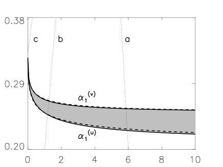
FIG. 5.: Shaded region shows the numerically-found existence region for three-wave solitons; analytically calculated boundaries (30) are plotted with dashed lines. Dotted lines (a,b,c) show dependence of the normalized mismatches on the propagation constant $\lambda$ for $\beta_{1}=-4$ and $\beta=10,-15,-25$ respectively. Parameters are $\chi=1/3$ and $\sigma=2$.

To understand the features of the three-wave solitons, we now recall that solutions of the original system (18) constitute a one-parameter family, as follows from Eqs. (19). Then, according to Eq. (21), a change of the propagation constant $\lambda$ corresponds to motion along a straight line in the parameter space $(\alpha,\alpha_{1})$. The limiting point for $\lambda\rightarrow+\infty$ is $(2\sigma,1)$, which always lies above the three-wave existence region. Thus, we find that the trajectory will go through this region only if $\beta_{1}<0$ and $\beta>2\sigma\beta_{1}/(1-\chi)$. Note that for fixed $\beta_{1}$ the value of $\beta$ determines the inclination angle, as demonstrated in Fig. 5 by the lines (a,b). On the other hand, line (c) corresponds to the case when the specified conditions do not hold, i.e. three-wave trapping is not possible for any $\lambda$. From this analysis it follows that the three-wave soliton always bifurcates from a two-wave state with $v=0$, and then transforms into the other two-wave mode with $u=0$. This process can be easily seen in Fig. 6, where examples of the power dependence on the propagation constant are shown.

FIG. 6.: Dependence of the total soliton power $P$ on the propagation constant. Parameter values for the plots (a,b) are the same as in Fig. 5 for the trajectories (a,b), respectively. In both cases, a three-wave soliton (solid line) bifurcates from two-wave solutions with $v=0$ (dotted) or $u=0$ (dashed). Crosses show approximate analytical results.

The plots in Fig. 6 demonstrate that the analytical solution gives a very precise estimate for the total power. It also accurately describes the soliton profiles in a wide region of mismatches, with an example being shown in Fig. 7. A thorough qualitative comparison is, however, a separate task, as there exist several parameters which control the mutual trapping. It will be presented elsewhere.

To summarize, we have analyzed three-wave solitons in an anisotropic medium. Our approach allowed us to predict corresponding parameter regions, and power dependence with high accuracy. Of course, some interesting aspects remain to be investigated, such as stability, formation of linear tails, and properties of higher-order modes. These problems are topics of separate study and thus will not be addressed here, but the results obtained form a background for further in-depth investigations.

FIG. 7.: Three-wave soliton profiles. Left: FF components ($u_{0}(x)$ – dotted, and $v_{0}(x)$ – dashed). Right: SH envelope. Crosses give analytically-calculated amplitudes. Parameters are the same as in Fig. 6(a), and $\lambda=5.35$.

III Two-dimensional solitons

Two-wave parametric spatial solitons can exist both in planar waveguides and in bulk nonlinear media [4]. In the latter case, the interaction between the FF and SH waves is described by the following system of coupled equations [7, 16, 23, 24]:

$$\begin{array}[]{l}{\displaystyle i\frac{\partial u}{\partial z}+\frac{\partial^{2}u}{\partial x^{2}}+\frac{\partial^{2}u}{\partial y^{2}}+u^{*}w=0,}\\[9.0pt] {\displaystyle i\sigma\frac{\partial w}{\partial z}+\frac{\partial^{2}w}{\partial x^{2}}+\frac{\partial^{2}w}{\partial y^{2}}-\beta w+\frac{1}{2}u^{2}=0,}\end{array}$$ (31)

where $x$ and $y$ are the transverse coordinates. Other variables and parameters are the same as for the (1+1) dimensional case described by Eqs. (1), with the obvious difference that the amplitudes depend on three coordinates, $u=u(x,y,z)$ and $w=w(x,y,z)$. We consider a spatial case close to the phase matching, i.e. $\sigma\simeq 2$.

Our goal in this section is to calculate the soliton envelopes by extending the method introduced for a planar case. Specifically, we look for circularly-symmetric stationary solutions of Eqs. (31), which can be found with the help of the following substitution:

$$\begin{array}[]{l}{\displaystyle u(x,y,z)=\lambda u_{0}\left(r\sqrt{\lambda}\right)e^{i\lambda z},}\\[9.0pt] {\displaystyle w(x,y,z)=\lambda w_{0}\left(r\sqrt{\lambda}\right)e^{2i\lambda z},}\end{array}$$ (32)

where $r=\sqrt{x^{2}+y^{2}}$ is the radial distance in cylindrical coordinates, and $u_{0}(r)$ and $w_{0}(r)$ are the real normalized envelope functions. Then, Eqs. (31) reduce to

$$\begin{array}[]{l}{\displaystyle\frac{d^{2}u_{0}}{dr^{2}}+\frac{1}{r}\frac{du_{0}}{dr}-u_{0}+u_{0}w_{0}=0,}\\[9.0pt] {\displaystyle\frac{d^{2}w_{0}}{dr^{2}}+\frac{1}{r}\frac{dw_{0}}{dr}-\alpha w_{0}+\frac{1}{2}u_{0}^{2}=0,}\end{array}$$ (33)

where the propagation constant $\lambda$ and the normalized mismatch $\alpha$ are introduced in the same way as in Eqs. (2),(3). Then, the soliton power and Hamiltonian are expressed via the the normalized values as:

$$P=\lambda P_{0},\,H=\lambda^{2}(H_{0}-P_{0}),$$ (34)

where $P_{0}=P_{u_{0}}+2\sigma P_{w_{0}}$, and

$$\begin{array}[]{rl}{\displaystyle P_{u_{0}}=2\pi\int_{0}^{+\infty}}&{\displaystyle u_{0}^{2}\;rdr,\,P_{w_{0}}=2\pi\int_{0}^{+\infty}w_{0}^{2}\;rdr,}\\[9.0pt] {\displaystyle H_{0}=2\pi\int_{0}^{+\infty}}&{\displaystyle{\left[{\left(\frac{\partial u_{0}}{\partial r}\right)}^{2}+{\left(\frac{\partial w_{0}}{\partial r}\right)}^{2}+\right.}}\\[9.0pt] &{\displaystyle\,{\left.+u_{0}^{2}+\alpha w_{0}^{2}-{u_{0}^{2}w_{0}}\right]}\;rdr.}\end{array}$$ (35)

Similarly to the one-dimensional case, Eqs. (33) are not integrable, and approximate soliton profiles were found using a variational method. Solutions were obtained for trial functions with Gaussian profiles (SGP) and described dependence of the Hamiltonian and power on mismatch $\alpha>0$ with a reasonable accuracy [16]. The limitations of the SGP remain the same – rough matching of actual profiles and inadequate description of the soliton tails. In order to construct a better solution, we have to start with some approximate scaling property of the soliton family. The problem is that effective ‘dissipation’ terms $\left(\sim\frac{1}{r}\frac{d}{dr}\right)$ in Eqs. (33) lead to: (i) distortion of soliton profiles in the center and (ii) higher far field localization, which, taken together, result in very complicated scaling features. This makes a general analysis quite difficult, and thus we limit our study to mismatches $\alpha>1$. It has been shown that in this parameter range the FF and SH relative beam width changes do not exceed a factor of two [16, 24]. On the other hand, from the structure of Eqs. (33), it follows that the balance between the second-order and effective dissipation linear terms, which affects the soliton shape, depends mainly on same characteristic beam width. Thus, we can assume that, to some extent, the SH envelope form stays almost intact for $\alpha>1$, and the trial function is

$$w_{0}(x)=w_{s}F\left(b_{s}r\right),$$ (36)

where the function $F$ describes a characteristic SH profile, and the relative amplitude $w_{s}$, together with the inverse width $b_{s}$, are scaling parameters. Then, we assume that, similarly to the (1+1)D case (10), the FF profile can be approximately described as

$$u_{0}(x)=u_{s}F^{p}{\left(b_{s}r\right)},$$ (37)

where $p$ is an unknown parameter.

To determine the SH characteristic profile, we consider a mismatch $\alpha=1$. This case is easier to analyze, as the envelopes of both mutually trapped components coincide, $w_{0}(r)=u_{0}(r)/\sqrt{2}=F(r)$. Here the function $F(r)$ satisfies the following equation

$$\frac{d^{2}F}{dr^{2}}+\frac{1}{r}\frac{dF}{dr}-F+F^{2}=0,$$ (38)

whose approximate solution was found earlier with the help of a Hartree-like approach [23]. However, here we choose to use a variational method in order to select the one which provides better matching. First, we present Eq. (38) in a variational form:

$$\frac{\delta L}{\delta F}=0,$$ (39)

where $\delta$ denotes the variational derivative, and $L$ is the Lagrangian corresponding to the original Eq. (38):

$$L(F)=\int_{0}^{+\infty}{\left[{\left(\frac{dF}{dr}\right)}^{2}+F^{2}-\frac{2}{3}F^{3}\right]}r\;dr.$$ (40)

Next, we select a trial function in the form

$$F_{0}(r)=F_{m}{\rm sech}^{2}(b_{0}r),$$ (41)

assuming that the profile is more or less close to that of planar solitons (8). Now we note that, according to (39), the Lagrangian reaches a minimum at an exact solution, and thus, to determine the peak amplitude $F_{m}$ and inverse width $b_{0}$ in the approximate expression (41), an extremum point of the $L(F_{0})$ integral should be found: ${\partial L(F_{0})}/{\partial F_{m}}={\partial L(F_{0})}/{\partial b_{0}}=0$. Solving these equations, we obtain the parameter values:

$$\begin{array}[]{l}{\displaystyle F_{m}=\frac{15\left(4\ln 2-1\right)}{32\ln 2-11}\approx 2.3781,}\\[18.0pt] {\displaystyle b_{0}=\frac{1}{2}\sqrt{\frac{5\left(4\ln 2-1\right)}{8\ln 2+1}}\approx 0.5818.}\end{array}$$ (42)

We made a comparison between the exact numerical and approximate solutions of Eq. (38) given by Eqs. (41),(42) and the Hartree approximation [23], and found that our result provides a much better matching. Thus, solution (41),(42) will be used in further calculation. In particular, we derive an approximate expression for the derivative $dF/dr$, which will be useful in further analysis:

$${\left(\frac{dF}{dr}\right)}^{2}\simeq 4b_{0}^{2}F^{2}{\left(1-\frac{F}{F_{m}}\right)}.$$ (43)

Now, after learning some important properties of the characteristic SH profile, the next step is to determine parameters in the trial functions (36,37). First, we substitute these expressions into the equation for the FF component in system (33). The resulting equality can’t be satisfied exactly for any $r$, but we can use Eq. (43) and get approximate relations between the parameters:

$$\begin{array}[]{l}{\displaystyle pb_{s}^{2}\left[1+4b_{0}^{2}\left(p-1\right)\right]=1,}\\[9.0pt] {\displaystyle pb_{s}^{2}\left[1+4b_{0}^{2}\left(p-1\right)F_{m}^{-1}\right]=w_{s},}\end{array}$$ (44)

Next, we fulfill the SH equation from (33) at $r\rightarrow 0$, and obtain:

$$w_{s}b_{s}^{2}{\left(1-F_{m}\right)}-\alpha w_{s}+\frac{1}{2}u_{s}^{2}F_{m}^{2p-1}=0.$$ (45)

To determine the solution parameters, one more relation is needed, preferably following from a conservation law, as this allows us to better describe far-field asymptotics. The difficulty here is that the equivalent dynamical system described by Eqs. (33) is dissipative, and thus is not Hamiltonian. However, it is still possible to derive a condition similar to Eq. (12) for a planar configuration. To calculate an integral relation, we substitute approximate profiles (36,37) into the equation for the SH component in (33), multiply the equality by $dF(b_{s}r)/dr$, and integrate over $(0,+\infty)$. The resulting expression contains an averaged dissipation term, which can be found using Eq. (38)

$\displaystyle\int_{0}^{+\infty}{\left(\frac{dF}{dr}\right)}^{2}\frac{dr}{r}=\frac{1}{3}F_{m}^{3}-\frac{1}{2}F_{m}^{2},$

and then the final equality is

$$w_{s}b_{s}^{2}{\left(\frac{1}{2}-\frac{1}{3}F_{m}\right)}-\frac{1}{2}\alpha w_{s}+\frac{1}{4p+2}u_{s}^{2}F_{m}^{2p-1}=0.$$ (46)

Now all the parameters can be determined from the derived relations. First, $p$ is found as a solution of cubic equation:

$$\begin{array}[]{l}{\displaystyle 8\alpha b_{0}^{2}p^{3}+2\alpha\left(1-6b_{0}^{2}\right)p^{2}+\left[\left(4/3\right)F_{m}-2\right.}\\[9.0pt] {\displaystyle\,\,\left.+\alpha\left(4b_{0}^{2}-1\right)\right]p+\left[1-\left(4/3\right)F_{m}\right]=0,}\end{array}$$ (47)

and then it is straightforward to calculate $b_{s}$, $w_{s}$, and $u_{s}$ one after another, employing Eqs. (44,45). Finally, using approximate expressions (41,42) for the wave profiles at $\alpha=1$ and scaling transformations Eqs. (36,37), the solution can be written as:

$$\begin{array}[]{l}{\displaystyle u_{0}(x)=u_{m}{\rm sech}^{2p}(xb),}\\[9.0pt] {\displaystyle w_{0}(x)=w_{m}{\rm sech}^{2}(xb),}\end{array}$$ (48)

where $u_{m}=u_{s}F_{m}^{p}\sqrt{2}$, $w_{m}=w_{s}F_{m}$, and $b=b_{s}b_{0}$. The amplitudes, characteristic widths, and scaling parameter $p$ are monotonic functions of $\alpha$, and for $1\leq\alpha<+\infty$ change in the limits: $1\geq p>1/2$, $b_{0}\leq b<\sqrt{2b_{0}^{2}/(1-2b_{0}^{2})}\approx 1.448$, $(F_{m}\sqrt{2}\approx 3.363)\leq u_{m}<+\infty$, $F_{m}\leq w_{m}<(F_{m}-2b_{0}^{2})/(1-2b_{0}^{2})\approx 5.267$. Keep in mind however, that, unlike the (1+1)D case, the asymptotics for large $\alpha$ are not exact.

It is interesting to note that solution (48), describing the soliton profiles in bulk media, reduces to expressions (13) for the (1+1)D case if the parameters characterizing the wave envelopes at $\alpha=1$ are chosen according to Eq. (6) as $F_{m}=3/2$ and $b_{0}=1/2$.

To study the accuracy of our solution, we made comparisons with direct numerical calculations. The results are summarized in Fig. 8 in the same way as for solitons in planar structures (see Fig. 2).

FIG. 8.: Comparison between exact numerical and approximate solutions, (48) and SGP, for solitons in bulk media. The characteristics shown are the same as in Fig. 2.

We also look at relative deviations, defining them in a way similar to (16) as:

$$\begin{array}[]{l}{\displaystyle\delta_{u}=\ln{\frac{\int_{-\infty}^{+\infty}{\left|u_{0}^{\rm exact}-u_{0}^{\rm approx.}\right|}^{2}rdr}{\int_{-\infty}^{+\infty}{\left|u_{0}^{\rm exact}\right|}^{2}rdr}},}\\[15.0pt] {\displaystyle\delta_{w}=\ln{\frac{\int_{-\infty}^{+\infty}{\left|w_{0}^{\rm exact}-w_{0}^{\rm approx.}\right|}^{2}rdr}{\int_{-\infty}^{+\infty}{\left|w_{0}^{\rm exact}\right|}^{2}rdr}}.}\end{array}$$ (49)

Each corresponding dependence is shown in Fig. 9(c) for our solution (48) on the left, and the SGP on the right. From the data presented, it follows that analytical solution (48) provides a very good approximation for both integral characteristics and soliton profiles [see also plots on the left in Figs. 9(a) and 9(b)]. Especially accurate results are observed for mismatches of the order $\alpha$ of $10^{0}$ to $10^{1}$. This range actually corresponds to interesting cases from an experimental point of view, as usually solitons are observed more or less close to phase matching, i.e. $\alpha\sim 2\sigma\simeq 4$ [1, 4]. The amazing precision is due to the fact that the approximate profile (41,42) provides outstandingly good matching with the exact envelope, as shown in Fig. 9(a). Actually, it can be claimed that this is an ’almost exact’ solution at $\alpha=1$ for solitons in a bulk medium, as the deviations $\delta_{u}$ and $\delta_{w}$ become extremely small [see the left plot in Fig. 9(c)]. Note also that the approximation coefficients in [23] are not nearly as accurate as those given in (42).

FIG. 9.: Comparison of numerical results with analytical predictions for (2+1)D soliton profiles given by: Eq. (48) on the left, and the SGP on the right. (a,b) Envelopes at $\alpha=1$ and $\alpha=10$ correspondingly. (c) Deviations of approximate profiles as defined in Eq. (49). Notation is the same as in Fig. 3.

For larger mismatches, i.e. $\alpha>10^{1}$, the deviations increase, but the errors always remain smaller than for the SGP. If even more accurate results are needed, it should be possible to start the derivation with the NLSE in the limit $\alpha\rightarrow+\infty$, and then take into account terms of order $\alpha^{-1}$. As for the opposite case, $\alpha<1$, linear tails may be expected to form, similarly to a (1+1)D configuration. However, such special analysis is beyond the scope of current paper, and we believe that these open problems will be addressed in further studies.

IV Concluding remarks

We have studied the properties of two- and three-component quadratic bright solitons in planar waveguides and in bulk media. Very accurate, yet simple and compact, approximate solutions have been derived to describe the actual wave profiles, with a precision which the previously-known approximations could not achieve. Such amazingly good results have been obtained because the trial functions were chosen to correspond to the scaling properties of the solitons. With the help of a specially-developed approach, the optimal values of fitting parameters have been found in a simple explicit form, which wouldn’t be possible with the variational method.

In particular, an ’almost exact’ solution has been derived which describes a whole family of two-wave planar solitons, accounting for all the key properties. It not only provides perfect estimations for integral characteristics (power and Hamiltonian), but also closely matches the envelope profiles of both components for any mismatch. On the other hand, the solution allowed us to reveal the existence of non-oscillating linear tails, and rigorously describe their features, which for example made it possible to explain and predict some peculiarities of multi-soliton bound states.

We also considered three-wave coupling in an anisotropic medium between the orthogonally-polarized FF and SH components. Mismatch values, when the three wave solitons can exist, have been determined analytically, and bifurcation scenarios have been described. Additionally, an approximate solution for soliton profiles has been obtained, and it provides close estimations in a wide parameter region.

Quite interesting results have been obtained for the case of solitons in a bulk medium. Although exact analytical expressions for the two-wave profiles in a (2+1) dimensional case are not known, even in simpler limiting cases (e.g., in the cascading limit the resulting single component NLSE is not integrable), we have been able to derive an ’almost exact’ solution for a specific mismatch value. General approximate expressions are also presented, giving very close matching in a wide range of detunings, covering values close to phase matching, which are of major interest from the experimental perspective.

REFERENCES

- [1] For a comprehensive review, see G. Stegeman, D.J. Hagan, and L. Torner, Opt. Quantum Electron. 28, 1691 (1996).
- [2] M. Georgieva-Grosse and A. Shivarova, p. 319; V.M. Agranovich and A.M. Kamchatnov, p.277, in Advanced Photonics with Second-Order Optically Nonlinear Processes, edited by A.D. Boardman, L. Pavlov, and S. Tanev, Eds. (Kluwer, Dordretch, 1998)
- [3] P.D. Drummond, K.V. Kheruntsyan, and H. He, Phys. Rev. Lett. 81, 3055 (1998).
- [4] For an overview of quadratic spatial solitons, see L. Torner, in Beam Shaping and Control with Nonlinear Optics, F. Kajzer and R. Reinisch, Eds. (Plenum, New York, 1998), p. 229; Yu.S. Kivshar, in Advanced Photonics with Second-Order Optically Nonlinear Processes, A.D. Boardman, L. Pavlov, and S. Tanev, Eds. (Kluwer, Dordretch, 1998), p. 451.
- [5] D. Anderson, Phys. Rev. A 27, 3135 (1983).
- [6] A. Ankiewicz, N. Akhmediev, G.D. Peng, and P.L. Chu, Opt. Comm. 103, 410 (1993).
- [7] Yu.N. Karamzin and A.P. Sukhorukov, Pis’ma Zh. Eksp. Teor. Fiz. 20, 734 (1974) [JETP Lett. 20, 339 (1974)]; Zh. Eksp. Teor. Fiz. 68, 834 (1975) [Sov. Phys. JETP 41, 414 (1976)].
- [8] Yu.N. Karamzin, A.P. Sukhorukov, and T.S. Filipchuk, Vest. Mosk. Univ. 33, 73 (1978) [Moscow Univ. Phys. Bull. 19, 91 (1978)].
- [9] A.V. Buryak and Yu.S. Kivshar, Opt. Lett. 19, 1612 (1994); 20, 1080(E) (1995); Phys. Lett. A 197, 407 (1995).
- [10] A.A. Kanashov and A.M. Rubenchik, Physica D 4, 122 (1981).
- [11] L. Torner, C.R. Menyuk, and G. Stegeman, Opt. Lett. 19, 1615 (1994); L. Torner, Opt. Comm. 114, 136 (1995).
- [12] H. He, M.J. Werner, and P.D. Drummond, Phys. Rev. E 54, 896 (1996).
- [13] D.E. Pelinovsky, A.V. Buryak, and Yu.S. Kivshar, Phys. Rev. Lett. 75, 591 (1995).
- [14] M.J. Werner and P.D. Drummond, Opt. Lett. 19, 613 (1994).
- [15] L. Bergé, V.K. Mezentsev, J.J. Rasmussen, and J. Wyller, Phys. Rev. A 52, R28 (1995).
- [16] V.V. Steblina, Yu.S. Kivshar, M. Lisak, and B.A. Malomed, Opt. Commun. 118, 345 (1995).
- [17] A.D. Boardman, K. Xie, and A. Sangarpaul, Phys. Rev. A 52, 4099 (1995).
- [18] V.M. Agranovich et al., Phys. Rev. B 53, 15451 (1996); V.M. Agranovich et al., Phys. Rev. E 55, 1894 (1997); C. Balslev Clausen, P.L. Christiansen, and L. Torner, Opt. Comm. 136, 185 (1997).
- [19] A.V. Buryak, Phys. Rev. E 52, 1156 (1995).
- [20] D. Mihalache, F. Lederer, D. Mazilu, and L.-C. Crasovan, Opt. Eng. 35, 1616 (1996).
- [21] A.C. Yew, A.R. Champneys, and P.J. McKenna, J. Nonlinear Sci. 9, 33 (1999).
- [22] Yu.S. Kivshar, A.A. Sukhorukov, and S.M. Saltiel, Two-color multistep cascading and parametric soliton-induced waveguides, to be published; e-print patt-sol/9905002.
- [23] K. Hayata and M. Koshiba, Phys. Rev. Lett. 71, 3275 (1993); 72, 178(E) (1994).
- [24] A.V. Buryak, Yu.S. Kivshar, and V.V. Steblina, Phys. Rev. A 52, 1670 (1995).