Stratified spatiotemporal chaos in anisotropic reaction-diffusion systems

Abstract

Numerical simulations of two dimensional pattern formation in an anisotropic bistable reaction-diffusion medium reveal a new dynamical state, stratified spatiotemporal chaos, characterized by strong correlations along one of the principal axes. Equations that describe the dependence of front motion on the angle illustrate the mechanism leading to stratified chaos.

Pattern formation in nonequilibrium systems has been extensively studied in isotropic, two-dimensional media CroHo . Among the most prominent experimental examples are Rayleigh-Benard convection and the Belousov-Zhabotinsky reaction in the contexts of fluid dynamics and chemical reactions respectively. Recently, there has also been considerable interest in systems with broken rotational symmetry, like convection in liquid crystals KraPe and chemical waves in catalytic surface reactions ImbErtl . Experimental and theoretical studies of such anisotropic systems showed novel phenomena like ordered arrays of topological defects chevrons , anisotropic phase turbulence Faller , reaction-diffusion waves with sharp corners corners , and traveling wave fragments along a preferred orientation MertPRE . Anisotropy is also often present in pattern formation processes in biological media, e.g. in cardiac tissue cardiac .

In this Letter we present a new dynamical state that is possible only in anisotropic media - stratified spatiotemporal chaos. We demonstrate the phenomenon with numerical simulations of the bistable FitzHugh-Nagumo equations with anisotropic diffusion and characterize it by computing orientation dependent correlation functions. In addition, an equation for the dependence of front velocities on parameters, curvature, and the angular orientation is derived. The mechanism leading to stratified chaos is described in terms of these analytic results. It is tightly linked to the anisotropy of the system and differs from the mechanism leading to spiral chaos in isotropic bistable media LeePRE ; HaMe94 ; HaMe97 . The findings here are relevant to catalytic reactions on surfaces where anisotropy is naturally provided by crystal symmetry and in biological tissue where anisotropy comes from fiber orientation.

Many qualitative features of pattern formation in chemical and biological reaction-diffusion systems are well described by FitzHugh-Nagumo (FHN) type models for bistable media IMN89 ; HaMeNL . The specific model we choose to study is

$$\frac{\partial u}{\partial t} = \epsilon^{-1}(u-u^{3}-v)+\delta^{-1}\nabla^{2}u+\frac{\partial}{\partial y}\bigl{[}d\delta^{-1}\frac{\partial u}{\partial y}\bigr{]}\,,$$

$$\frac{\partial v}{\partial t} = u-a_{1}v-a_{0}+\nabla^{2}v\,,$$ (1)

where $u$ is the activator and $v$ the inhibitor. The parameters $a_{1}$ and $a_{0}$ are chosen so that Eqs. (1) represent a bistable medium with two stationary and uniform stable states, an “up” state, $(u_{+},v_{+})$, and a “down” state, $(u_{-},v_{-})$. Front solutions connect the two states. The number of front solutions changes, when a single front (an “Ising” front) that exists for values of $\eta:=\sqrt{\epsilon\delta}>\eta_{c}$ loses stability to a pair of counter-propagating fronts (“Bloch” fronts) for $\eta\leq\eta_{c}$. The corresponding bifurcation is referred to as the nonequilibrium Ising-Bloch (NIB) bifurcation, hereafter the “front bifurcation.” The anisotropy of the medium is reflected through the parameter $d$.

Figure 1 shows the formation and time evolution of stratified chaos obtained by numerical solution of Eqs. (1). The initial state is isotropic spiral chaos. As time evolves a clear orientation of up-state (grey) domains along the $y$ direction develops. The domains consist primarily of elongating stripe segments which either merge with other segments or shorten by emitting traveling blobs. The stratified chaos state is robust and develops from a variety of initial conditions including a single spot.

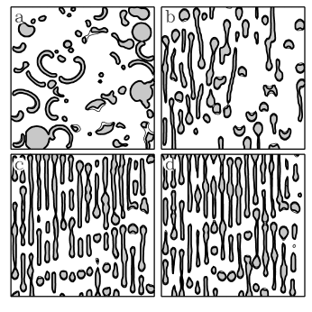
Figure 1: The development of stratified spatio-temporal chaos from an initial state of isotropic spatio-temporal chaos. The thick contour line represents $u=0$ and the thin contour line $v=0$. The shaded regions are up-state domains. Parameters: $a1=2.0$, $a_{0}=-0.1$, $\epsilon=0.039$, $\delta=1.7$, $d=1.0$, $x=[0,80]$, $y=[0,80]$.

To gain insight we have followed the dynamics of $u$ and $v$ along the $x$ and $y$ axes and display them in the form of space-time plots in Fig. 2. A nearly periodic non-propagating pattern along the $x$ axis and irregular traveling wave phenomena along the $y$ axis are observed. A characteristic property of spatio-temporal chaotic patterns are correlations that decay on a length scale $\xi$ much smaller than the system length $L$. We have computed the normalized spatial two-point correlation functions, $C_{y}(r)$ and $C_{x}(r)$, for the $u$ field in both the $x$ and $y$ directions, where $C_{y}(r)=<\Delta u(x,y+r)\Delta u(x,y)>/<\Delta u(x,y)^{2}>$, $C_{x}(r)=<\Delta u(x+r,y)\Delta u(x,y)>/<\Delta u(x,y)^{2}>$, $\Delta u(x,y)=u(x,y)-<u>$, and the brackets $<>$ denote space and time averaging. Figure 3 shows the results of these computations. Correlations in the $y$ direction decay fast to zero, whereas correlations in the $x$ direction oscillate with constant amplitude. This observation may be used to define stratified chaos as a state that displays finite correlation length in one direction ($x$) and infinite correlation length in the other ($y$).

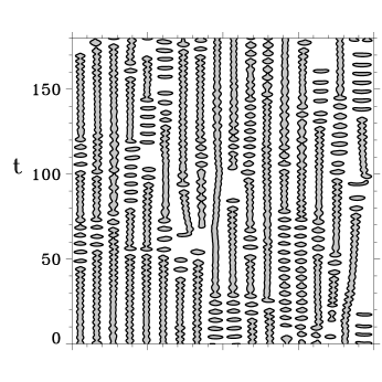
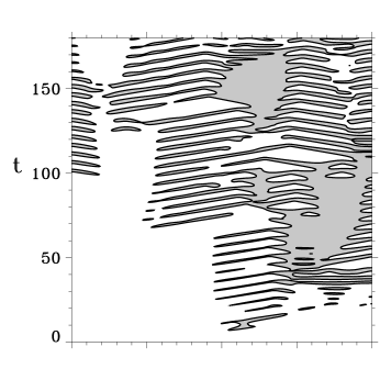
Figure 2: Space-time plots of cuts parallel to the $x$ axis (top) and the $y$ axis (bottom) for the simulation of Fig. 1. The nearly vertical columns on the top figure show instances of periodic breathing motion of stripe segments (modulated continuous segments) and periodic blob formation (spot arrays).

An important analytical tool for studying front dynamics consists of relations between the normal front velocity $C_{n}$ and other front properties like curvature. Relations of that kind have successfully been used in the study of pattern formation in isotropic media HaMe94 , and we wish to exploit this tool for anisotropic media as well.

Figure 3: Correlation functions $C_{x}(r)$ (solid curve) and $C_{y}(r)$ (dashed curve).

Velocity-curvature relations are derived here for $\lambda:=\sqrt{\epsilon/\delta}\ll 1$. The first step in this derivation is to define an orthogonal coordinate system $(r,s)$ that moves with the front, where $r$ is a coordinate normal to the front and $s$ is the arclength. We denote the position vector of the front by ${\bf X}(s,t)=(X,Y)$, and define it to coincide with the $u=0$ contour line. The unit vectors tangent and normal to the front are given by ${\bf\hat{s}}=\cos\theta{\bf\hat{x}}+\sin\theta{\bf\hat{y}}$ and ${\bf\hat{r}}=-\sin\theta{\bf\hat{x}}+\cos\theta{\bf\hat{y}}$, respectively, where $\theta(s,t)$ is the angle that $\hat{s}$ makes with the $x$ axis. A point ${\bf x}=(x,y)$ in the laboratory frame can be expressed as ${\bf x}={\bf X}(s,t)+r{\bf\hat{r}}$. This gives the following relations between the laboratory coordinates $(x,y)$ and the coordinates $(s,r)$ in the moving frame: $x=X(s,t)-r\sin\theta(s,t)$, and $y=Y(s,t)+r\cos\theta(s,t)$ where we defined ${\bf\hat{s}}=\partial{\bf X}/\partial s$ and ${\partial X}/{\partial s}=\cos\theta$, ${\partial Y}/{\partial s}=\sin\theta$. In terms of the moving frame coordinates the front normal velocity and curvature are given by $C_{n}=-{\frac{\partial r}{\partial t}}$ and $\kappa=-\frac{\partial\theta}{\partial s}$, respectively.

The second step is to express Eqs. (1) in the moving frame and use singular perturbation theory, exploiting the smallness of $\lambda$. We distinguish between an inner region that includes the narrow front structure, and outer regions on both sides of the front. In the inner region $\partial u/\partial r\sim{\cal O}(\lambda^{-1})$ and $\partial v/\partial r\sim{\cal O}(1)$. In the outer regions both $\partial u/\partial r$ and $\partial v/\partial r$ are of order unity. In the inner region $v=v_{f}$ is taken to be constant. Expanding both $u$ and $v_{f}$ as powers series in $\lambda$ and using these expansions in the moving frame equations we obtain, at order ${\cal O}(\lambda)$, a solvability condition that leads to the equation

$$C_{n}=-{\frac{3}{\eta\sqrt{2}}}I(\theta)v_{f}-\frac{1+d}{\delta I(\theta)^{2}}\kappa\,,$$ (2)

where $I(\theta)=\sqrt{1+d\cos^{2}\theta}$. In the outer regions to the left and to the right of the front region different approximations can be made. Here $\frac{\partial u}{\partial r}\sim\frac{\partial v}{\partial r}\sim{\cal O}(1)$ and to leading order all terms that contain the factor $\lambda$ can be neglected. The resulting equations can be solved for $v$ in the two outer regions. Continuity of $v$ and of $\frac{\partial v}{\partial r}$ at the front position $r=0$ yield a second relation between $C_{n}$ and $v_{f}$. Eliminating $v_{f}$ by inserting this relation into Eq. (2) gives an implicit relation between the normal velocity of the front and its curvature

$$C_{n}+\frac{1+d}{\delta I(\theta)^{2}}\kappa=\frac{3I(\theta)(C_{n}+\kappa)}{\eta\sqrt{2}q^{2}\sqrt{(C_{n}+\kappa)^{2}+4q^{2}}}+\frac{3I(\theta)a_{0}}{\eta\sqrt{2}q^{2}}\,,$$ (3)

where $q^{2}=a_{1}+1/2$. A complete account of this derivation will be published elsewhere.

Figures  4 display solutions of Eq. (3) showing the dependence of the front velocity on front curvature and propagation direction for the parameter values of Fig. 1. In Fig. 4a $C_{n}$ vs $\kappa$ relations are shown for two orthogonal propagation directions. In the $x$ direction, $\theta=\pi/2$ (dashed curve), there is only one planar front solution with negative velocity (a down-state invading an up-state), indicating an Ising regime. The negative slope of the $C_{n}$ $\kappa$ relation implies stability to transverse perturbations. In the $y$ direction, $\theta=0$ (solid curve), there are three planar front solutions indicating a Bloch regime. The positive-velocity front (up-state invading down-state) is unstable to transverse perturbations whereas the negative-velocity front is stable. The middle branch corresponds to an unstable front.

Figure 4: Two views of the relation  (3) corresponding to the parameters of the simulation in Figure 1. (a) The velocity-curvature relation for fronts in the $x$ direction (dashed curve) and $y$ direction (solid curve). (b) The velocity of planar ($\kappa=0$) fronts at different angles. Bloch fronts exist in narrow sectors around $\theta=0$ and $\theta=\pi$. The wider sectors in between correspond to Ising fronts.

Figure 4b shows the angular dependence of planar-front velocities. Counter-propagating (Bloch) fronts exist in a narrow sector around the $y$ direction ($\theta=0$). The other directions support only a single (Ising) front. The Ising front speed is smallest in the $x$ direction ($\theta=\pi/2$) and increases as $\theta$ deviates from $\pi/2$.

The dynamics of fronts as displayed in Fig. 1 are affected by curvature, propagation direction, and front interactions. Eq. (3) captures the effects of the first two factors but does not contain information about front interactions. The necessary information for our purpose can be summarized as follows.

The time evolution of a pair of fronts approaching one another is affected by the speed of non-interacting fronts and by the diffusion rate of the activator $u$ (assuming an inhibitor diffusion constant equal to unity as in Eqs. (1)). Consider a pair of fronts pertaining to up-states invading a down-state, propagating toward one another in an isotropic medium ($d=0$). If the distance between the fronts decreases below a critical value, $\lambda_{c}\sim{\cal O}(\sqrt{\epsilon/\delta})$, the two fronts collapse, leaving a uniform up-state. The accumulation of the inhibitor in the space enclosed by the fronts, however, slows their motion. If the (non-interacting) front speed is low enough, or if $\lambda$ is small enough, there is enough time for the inhibitor to slow the fronts down to a complete stop before they reach the critical distance $\lambda_{c}$. In that case the subsequent evolution depends on the front type. A pair of Ising fronts may either form a stationary pulse or, closer to the front bifurcation, a breathing pulse. A pair of Bloch fronts reflect and propagate away from one another HaMeNL . Thus, high front speed or fast activator diffusion ($\delta$ small and $\lambda_{c}$ large) lead to collapse, whereas low front speed and slow activator diffusion lead to strong front repulsion. A similar argument holds for down-state invading up-state fronts.

Returning to anisotropic media we need to know how the two factors that affect front interactions, front speed and activator diffusion, depend on the direction of propagation. The angular dependence of the front speed is already given in Fig. 4b. The angular dependence of the activator diffusion can be deduced by inspecting Eqs. (1). It is $1/\delta$ in the $x$ direction and $(1+d)/\delta$ in the $y$ direction. Since $d>0$ the activator diffusion constant increases as the propagation direction changes from the $x$ direction to the $y$ direction.

We can discuss now the mechanism of stratified chaos. As Fig. 4a shows, the $x$ direction represents a system that supports stationary or breathing planar stripe patterns. The $y$ direction represents a system where traveling waves prevail. The distinct characters of the medium along the two principal axes is reflected in the space-time plots of Fig. 2: nearly vertical columns in the $x$ direction indicate stationary or breathing motion, and diagonal stripes in the $y$ direction indicate traveling wave phenomena.

The irregular character of the dynamics comes from blob formation events as shown in Figure 5. The front speed and activator diffusion in the $x$ direction are sufficiently slow for Ising fronts to repel one another (rather than collapse). As the tip of the stripe segment grows outward and forms a bulge, propagation directions deviating from the $x$ direction develop. At these directions both the front speed and the activator diffusion are higher. As a result approaching fronts may collapse. This is exactly the blob pinching process in frames (c), (d) and (e) of Fig. 5. The process is periodic for extended periods of time as indicated by the vertical spot arrays in Fig. 2.

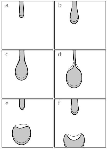
Figure 5: Close up of repeated blob formation. Shaded regions are up-state domains. Thick (thin) lines are $u=0$ ($v=0$) contours. The $v=0$ line always lags behind the $u=0$ line. The tip of a stripe segment (a) grows outward (b)-(c). A pinching dynamics begins (d) which leads to blob formation (e) traveling along the $y$ direction (f). The blob formation leaves a shortened stripe segment (e) whose tip grows outward again (f) and the process repeats. The parameters are the same as in Fig. 1.

In summary, stratified chaos relies on two main elements: (i) stationary or breathing domains vs traveling wave phenomena in orthogonal directions, and (ii) an angular dependence of front interactions that leads to blob formation. Without the second element stripe segments would merge to ever longer segments until a periodic stripe pattern is formed. These elements suggest the parameter regime where stratified chaos is expected to be found. The first element implies a regime along the front bifurcation such that there is stationary or breathing motion in the direction with faster activator diffusion and traveling waves in the other (slower diffusion) direction. The width of this regime increases with the anisotropy $d$. The second element implies that in the direction of breathing or stationary domains the system is close to the onset of breathing motion. Deviations from this direction which move the system toward the traveling wave regime then lead to front collapse. These expectations were verified numerically. Part of the work of U. T. was supported by grant D/98/14745 of the German Academic Exchange Board (DAAD). M. B. gratefully acknowledges the hospitality of Ben-Gurion University and support of the Max-Planck-Society (MPG) by an Otto-Hahn-Fellowship. Part of this research is supported by the Department of Energy, under contract W-7405-ENG-36.

References

- (1) M. C. Cross and P. C. Hohenberg, Rev. Mod. Phys. 65, 851 (1993).
- (2) L. Kramer and W. Pesch, Ann. Rev. Fluid. Mech. 27, 515 (1995).
- (3) R. Imbihl and G. Ertl, Chem. Rev. 95, 697 (1995).
- (4) M. Scheuring, L. Kramer and J. Peinke, Phys. Rev. E 58, 2018 (1998); G. D. Granzow and H. Riecke, Physica A 249, 27 (1998).
- (5) R. Faller and L. Kramer, Phys. Rev. E 57, 2649 (1998).
- (6) F. Mertens and R. Imbihl, Nature 370, 124 (1994); A. S. Mikhailov, Phys. Rev. E 49, 5875 (1994); N. Gottschalk, F. Mertens, M. Bär, M. Eiswirth and R. Imbihl, Phys. Rev. Lett. 73, 3483 (1994).
- (7) F. Mertens, N. Gottschalk, M. Bär, M. Eiswirth, A. Mikhailov and R. Imbihl, Phys. Rev. E 51, 5193 (1995).
- (8) A. T. Winfree, Int. J. Bif. Chaos 7, 784 (1997); J. Keener and J. Sneyd, Mathematical Physiology (Springer, New York, 1998).
- (9) K. J. Lee and H. L. Swinney, Phys. Rev. E 51, 1899 (1995); G. Li, Q. Ouyang and H. L. Swinney, J. Chem. Phys. 105, 10830 (1996).
- (10) A. Hagberg and E. Meron, Phys. Rev. Lett. 72, 2494 (1994); Chaos 4, 477 (1994).
- (11) A. Hagberg and E. Meron, Phys. Rev. Lett. 78, 1166 (1997); Physica D 123, 460 (1998).
- (12) H. Ikeda, M. Mimura and Y. Nishiura, Nonl. Anal. TMA 13, 507 (1989).
- (13) A. Hagberg and E. Meron, Nonlinearity 7, 805 (1994).