Renormalization study of two-dimensional convergent solutions of the porous medium equation

Abstract

In the focusing problem we study a solution of the porous medium equation $u_{t}=\Delta\left(u^{m}\right)$ whose initial distribution is positive in the exterior of a closed non-circular two dimensional region, and zero inside. We implement a numerical scheme that renormalizes the solution each time that the average size of the empty region reduces by a half. The initial condition is a function with circular level sets distorted with a small sinusoidal perturbation of wave number $k\geq 3$. We find that for nonlinearity exponents $m$ smaller than a critical value which depends on $k$, the solution tends to a self-similar regime, characterized by rounded polygonal interfaces and similarity exponents that depend on $m$ and on the discrete rotational symmetry number $k$. For $m$ greater than the critical value, the final form of the interface is circular.

1 Introduction

This work deals with solutions to the nonlinear diffusion equation

$$\frac{\partial u}{\partial t}=\Delta\left(u^{m}\right),$$ (1)

where $m>1$ is constant and $\Delta$ denotes the Laplace operator in $\mathbf{R}^{d}$. Equation (1) arises in various problems, such as the spreading of viscous gravity currents [13, 6], the diffusion of strong thermal waves [9], and the isentropic flow of an ideal gas in a homogeneous porous medium [4, 8]. In the latter application, $u$ represents the scaled density of the gas. For $m=1$ equation (1) is the classical heat conduction equation and there are other applications which involve values of $m<1$. One of the salient features of the “slow diffusion” case $m>1$ is the occurrence of interfaces moving with finite velocity, that separate empty regions where $u=0$ from regions where $u>0$. More detailed information about the properties of solutions to equation (1) can be found in [4].

In order to discuss the behavior of solutions to equation (1) it is convenient to replace the independent variable $u$ with

$$v=\frac{m}{m-1}u^{m-1}.$$

In the gas flow interpretation, $v$ represents the scaled pressure via the ideal gas law. If $u$ satisfies (1) then $v$ satisfies

$$\frac{\partial v}{\partial t}=(m-1)v\Delta v+\left|\nabla v\right|^{2},$$ (2)

where $\nabla$ is the gradient operator in $\mathbf{R}^{d}$.

Here we are interested in the focusing problem in which we solve equation (2) starting from an initial distribution which is positive in the exterior of a closed bounded region $D$ and zero inside $D$ (see Fig. 1). At some finite time $T>0$, called the focusing time, $v$ will for the first time be positive throughout the initially empty region $D$.

In [5] it is shown that for each $m\in\left(1,\infty\right)$ there is a unique similarity exponent $\beta(m,d)\in\left(\frac{1}{2},1\right)$ and a one-parameter family of functions $F_{c}$ such that the functions

$$v_{c}(x,t)=(T-t)^{2\beta-1}F_{c}\left(\frac{\left|x\right|}{(T-t)^{\beta}}\right).$$ (3)

with $\beta=\beta\left(m,d\right)$, are self-similar solutions to (2). Moreover, there exists a $\gamma(d,m)$ such that

$$F_{c}(\xi)\left\{\begin{tabular}[]{l}$=0$ for $0\leq\xi\leq\left(\frac{c}{\gamma}\right)^{\beta}$\\ $>0$ for $\xi>\left(\frac{c}{\gamma}\right)^{\beta}$\end{tabular}\right.,$$

where $\gamma=\gamma(d,m)$. Thus the $v_{c}(x,t)$ are focusing solutions to equation (2) with interfaces given by

$$\frac{\left|x\right|}{(T-t)^{\beta}}=\left(\frac{c}{\gamma}\right)^{\beta}.$$

The focusing problem is well studied in the radially symmetric case. In particular, it is proven in [1, 2] that some member of the Graveleau family (3) describes locally, to leading order, the focusing behavior of essentially any radially symmetric focusing solution to the pressure equation (2). The situation is much more complicated in the absence of radial symmetry. Physical experiments involving convergent gravity flows ($m=4,d=2$) followed by numerical experiments [7] indicate that both large and small deviations from rotational symmetry may be amplified as the flow tries to fill the hole. A formal linear stability analysis for general $m$ and $d$ (cf. [3] and Appendix 2) shows that the Graveleau solutions are indeed unstable, at least when $m$ is close to unity, and that the number of unstable modes increases as $m\searrow 1$. This suggests that a sequence of bifurcations occurs as $m$ decreases from $\infty$ to $1$. The existence of these bifurcations is proved in [3]. The bifurcating solutions are self-similar, but not axially symmetric. They are invariant with respect to the action of the group $O(d-1,\bf{R})$ of $(d-1)\times(d-1)$ real orthogonal matrices. In this paper we restrict our attention to the plane case $d=2$. In this case the results of [3] show that for any $\bar{m}\in(1,\infty)$ there exists an integer $k_{*}(\bar{m})\in(2,\infty)$ such that a symmetry breaking bifurcation from the radially symmetric Graveleau solutions occurs at some $m_{k}\in(1,\bar{m})$ for each $k>k_{*}(\bar{m})$. The bifurcating solutions are non-radial self-similar focusing solutions possessing $k$-fold symmetry, i.e., the symmetry of $\cos(k\theta)$. Numerical studies show that for each $k\geq 3$ the bifurcation point $m=m_{k}$ is unique so that the Graveleau solutions are linearly stable with respect to perturbations with $k$-fold symmetry for $m>m_{k}$ and unstable for $m_{k}>m>1$. Moreover, the $m_{k}$ are ordered

$$\infty>m_{3}>m_{4}>...>m_{k}>...\searrow 1.$$

Crude estimates for the first four $m_{k}$ are given in Table I (See also Table IV in Appendix 2).

k estimate

3 $$m_{3}\in(1.69,1.7)$$

4

5

6

Table I: Estimates of the values of $m_{k}$ for which the circular self-similar solution bifurcates into a non-circular solution.

The results in [3] give no information about stability with respect to perturbations with wave number $k=2$. The experimental and numerical results in [7] suggest instability. This is confirmed by numerical linear stability analysis which shows that the Graveleau interface is unstable with respect to perturbations with wave number 2 for all values of $m$. In particular, there appear to be no bifurcating branches of self-similar focusing solution with the 2-fold symmetry. We discuss this briefly in Section 5 of this paper and in more detail in reference [18].

In this paper we carry out detailed numerical studies of focusing solutions to equation (2) whose initial distributions have interfaces which are circles with small perturbations. Mainly, we deal with initial conditions whose interfaces are of the form

$$r=a\left(1+\varepsilon\cos(k\theta)\right)$$ (4)

with $\varepsilon\ll a$, although in Section 5 we will consider perturbations with mixed modes. By using a numerical renormalization technique inspired by the pioneering work of Chen and Goldenfeld [10, 11] we are able to follow the evolution of the interface to times very close to the focusing time. Thus we are able to obtain very detailed information about the asymptotic form of the solution as it focuses. As we shall see below, for single mode perturbations with $k$-fold symmetry, the numerical results indicate that the leading term in the focusing asymptotics is a self-similar solution of the form

$$v=(T-t)^{2\delta-1}V_{c}\left(\frac{r}{(T-t)^{\delta}},\theta\right)$$ (5)

where $c$ is a parameter, $\delta=\delta\left(k,m\right)$ is the similarity exponent, and $V_{c}$ satisfies

$$V_{c}(\zeta,\theta)=V_{c}(\zeta,\theta+\frac{2\pi n}{k})\mbox{ for }n=1,...,k-1.$$ (6)

Moreover, the focusing interface is asymptotically of the form

$$r=(T-t)^{\delta}A\left(\theta\right),$$

and $\delta\left(k,m_{k}\right)=\beta\left(2,m_{k}\right)$, where $\beta$ is the similarity exponent for the Graveleau solution and $m_{k}$ is the bifurcation point found in [3]. Therefore we conclude that the functions given by (5) are the bifurcating solutions found in [3].

2 Numerical scheme and renormalization procedure

In order to solve Eq. (2) numerically, we discretize a circular domain $D=[0,R]\times[0,2\pi/k]$ with a uniform polar grid of interval sizes $\delta r=R/N_{r}$ and $\delta\theta=2\pi/N_{\theta}$. The numerical solution is stored in a matrix as $v(r,\theta,t)=v_{ij}$ with $r=i\delta r$ and $\theta=j\delta\theta$. In order to integrate the PDE in time, we use an explicit Euler scheme

$$v_{ij}(t+\delta t)=v_{ij}(t)+\delta tH_{ij}$$ (7)

where $H_{ij}$ is a finite differences approximation of the derivatives of the right hand side of Eq. (2). We compute the derivatives of the term $\left|\nabla v\right|^{2}=v_{r}^{2}+v_{\theta}^{2}/r^{2}$ with a second order upwind ENO (essentialy non-oscillatory) scheme [14, 15] (see Appendix 1). This method guarantees that the numerical scheme will be able to describe accurately the discontinuities on the first derivative that spontaneously appear in the case $m=1$ (Hamilton-Jacobi limit) and at the interface. Due to the diffusive nature of the Laplacian term in Eq. (2), the corresponding derivatives are computed with standard centered second order approximations,

$$\Delta v=v_{rr}+\frac{v_{r}}{r}+\frac{v_{\theta\theta}}{r^{2}}\simeq$$ (8)

$$\simeq\frac{v_{i+1,j}-2v_{ij}+v_{i-1,j}}{\delta r^{2}}+\frac{v_{i+1,j}-v_{i-1,j}}{2\delta r\,r_{i}}+\frac{v_{i,j+1}-2v_{ij}+v_{i,j-1}}{\delta\theta^{2}r_{i}^{2}}.$$ (9)

Near the interface there is a discontinuity in the first derivative that may generate numerical errors when we compute the Laplacian with Eq. (9). Therefore, for the grid points $v_{ij}$ situated at a distance smaller than $2\delta r$ from the interface, the Laplacian is computed by linearly extrapolating in the variable $r$ the values of the Laplacian from the nodes of behind, which were previously computed with Eq. (9).

At the boundaries $\theta=\pm\pi/k$ we apply the boundary condition of periodicity $v(-\pi/k)=v(\pi/k)$. This is simply a convenience, since computations without this forced symmetry yield equivalent results. At the boundary $r=R$ we apply the boundary condition $v_{rr}=0$. This is equivalent to a first order linear extrapolation of the ghost points $v_{N_{r}+1,j}$ outside $R$, which are needed in order to compute the derivatives at $R$. Finally, at $r=0$ we set $v=0$.

We start the integration with a rather arbitrary initial condition,

$$v^{(0)}(r,\theta,t_{0})=r-a_{0}\left(1+\varepsilon\cos k\theta\right),\hskip 42.67912pt\varepsilon=0.1$$ (10)

which describes a function whose contour lines are perturbed circles, and which interface is given by Eq. (4). The exact form of the initial condition is not very critical, because the asymptotic solution only depends on $k$ (which determines the symmetry) and $m$, as was verified numerically.

We integrate the diffusion equation over a sequence of time intervals $(t_{n},t_{n+1})$ starting with $n=0$, and renormalize the solution at each right hand end point $t=t_{n+1}$ before continuing the integration. The renormalization times $t_{n+1}$ are taken to be the times when the average radius of the interface

$$\overline{a}(t)=\frac{1}{2\pi}\int_{0}^{2\pi}a(\theta,t)d\theta$$ (11)

reaches half of its initial value. The renormalized solution is defined to be

$$v^{(n+1)}(r,\theta,t_{n+1})=Z^{(n)}\cdot v^{(n)}(r/2,\theta,t_{n+1})$$ (12)

for $n=0,1,2,...$. This transformation is performed by linearly interpolating the values of the grid,

$$v_{ij}^{(n+1)}=Z^{(n)}\cdot v_{i/2,j}^{(n)}\hskip 28.45274pt\mbox{ for even }i$$

and

$$v_{ij}^{(n+1)}=Z^{(n)}\cdot(v_{i/2,j}^{(n)}+v_{i/2+1,j}^{(n)})/2\hskip 28.45274pt\mbox{ for odd }i.$$

The constant $Z^{(n)}$ is taken as the reciprocal of the maximum value of the function $v$ in the renormalized domain of integration

$$Z^{(n)}=\left(\max_{r\leq R/2}v^{(n)}(r,\theta,t_{n+1})\right)^{-1}.$$ (13)

The superscript $(n)$ indicates how many renormalizations we have made up to the time $t_{n+1}$. The errors introduced in the linear interpolation are of second order, the same as in the discretization of the derivatives. It is very important to determine the time $t_{n+1}$ accurately, and this is done by first detecting the exact time when the interface crosses half of its initial value at the previous renormalization, and then using this information to re-compute the time step $\delta t$ and the solution such that the interface reaches exactly the half of the initial value.

We summarize the procedure as follows:

1. Initialize $v^{(0)}(r,\theta,t_{0})$ with Eq. (10). Let $n=0$.

2. Starting from $t=t_{n}$ solve Eq. (2) with standard finite differences until the time $t=t_{n+1}$ where $\overline{a}(t_{n+1})=\overline{a}(t_{n})/2$. Here we have $v^{(n)}(r,\theta,t_{n+1})$.

3. Renormalize $v^{(n+1)}(r,\theta,t_{n+1})=Z^{(n)}\cdot v^{(n)}(r/2,\theta,t_{n+1}).$

4. While

   $$\varepsilon_{n}=\sqrt{\frac{1}{\pi(R/2)^{2}}{\int\int}_{r\leq R/2}\left|v^{(n+1)}(r,\theta,t_{n+1})-v^{(n)}(r,\theta,t_{n})\right|^{2}r\ dr\ d\theta}>\tau$$ (14)

   let $n=n+1$ and return to step 2.

where $\tau$ is a tolerance. In the experiments reported below, we have set $\tau=10^{-6}$.

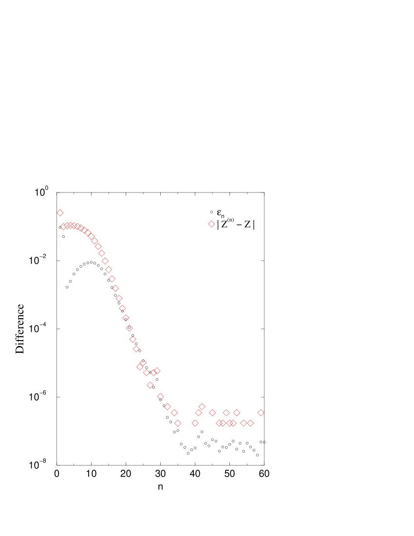
Figure 2: Convergence of the numerical solution: the difference between succesive approximations tend to zero and the renormalization constant $Z$ tends to a constant as the number of renormalizations $n$ increases. In this case $m=1.5$, $N_{r}=300$, $N_{\theta}=300$ and the initial shape is a perturbated circle with $k=3$.

We found that when we repeat this procedure $n$ times, the solution typically converges for $n\geq 50$. This convergence is a necesary condition for the existence of a self-similar solution. In Fig. (2) we show the convergence of the iterative procedure by plotting the difference of succesive approximations given by Eq. (14) and the departure of $Z^{(n)}$ from its asymptotic value.

In order to compute the exponent $\delta$ we note that once the scheme has converged,

$$v^{(n+1)}(r,\theta,t_{n+1})=v^{(n)}(r,\theta,t_{n})$$

and

$$Z^{(n+1)}=Z^{(n)}=Z$$

(here we are ignoring the numerical errors). Then, from Eq. (12),

$$v^{(n)}(r,\theta,t_{n})=Z\cdot v^{(n)}(r/2,\theta,t_{n+1}).$$ (15)

Thus, the solution at time $t_{n+1}$ is proportional to the solution at time $t_{n}$ with the distances scaled by a factor two.

By substituting $v$ from Eq. (5),

$$\left(-t_{n}\right)^{2\delta-1}V\left(\frac{r}{\left(-t_{n}\right)^{\delta}},\theta\right)=Z\left(-t_{n+1}\right)^{2\delta-1}V\left(\frac{r}{2\left(-t_{n+1}\right)^{\delta}},\theta\right)$$ (16)

(here we have put $T=0$) it is clear that

$$t_{n}=2^{1/\delta}t_{n+1}\hskip 28.45274pt\mbox{and }\hskip 28.45274pt\left(-t_{n}\right)^{2\delta-1}=Z\left(-t_{n+1}\right)^{2\delta-1}.$$ (17)

Solving these algebraic equations we find that the similarity exponent is given by

$$\delta^{-1}=\log_{2}\left(\frac{4}{Z}\right).$$ (18)

3 Validation

1. In order to show the accuracy of this numerical computation, we compare in Table II the numerical solution for the circularly symmetric case with the Graveleau solution, and we find a good agreement in the exponents ($\delta=\beta$ in this case, see Eqs. 3 and 5) .

   $$\begin{array}[]{ccc}m&Numeric&{}^{\prime}Exact^{\prime}\\ 1.0&1.00000&1\\ 1.1&0.976749&0.976744\\ 1.2&0.956533&0.956517\\ 1.3&0.938768&0.938756\\ 1.4&0.923066&0.923071\\ 1.5&0.909103&0.908983\\ 1.6&0.896595&0.896346\\ 1.7&0.885311&0.884940\\ 1.8&0.875052&0.874546\\ 1.9&0.865675&0.865052\\ 2.0&0.857052&0.856333\end{array}$$

   Table II: Exponents for the circular case, $R=1,N_{r}=300$

   This comparison checks the accuracy of the renormalization procedure and the temporal integration.

2. We also computed the solutions corresponding to the Hamilton-Jacobi case $m=1$, and we compared the numerical result with the exact solution. The interfaces of the exact solution are regular polygons of $k$ sides ($k\geq 3$), and the function $v$ is a set of $k$ planes of the form

   $$v(r,\theta,t)=c(x+a(t))=c(r\cos\theta+a(t))\hskip 28.45274pt-\pi/k\leq\theta<\pi/k$$ (19)

   $$v(r,\theta+2\pi n/k,t)=v(r,\theta,t)\qquad for\ n=1\,..\,k-1$$

   where $a(t)=ct$ and $c\$is a constant . The level lines are regular polygons and the similarity exponent is $\delta=1$. This solution exhibits a set of $k$ discontinuities in the derivatives at the apeses of the polygonal level sets. The level sets of the numerical solution are shown in Fig. 3 for $k=3,4,$ and $5$. The numerical solution gives the value of the exponent with an absolute error of the order of $10^{-5}$ when a discretization of $N_{r}=300$ and $N_{\theta}=300$ is used. The relative departure of the numerical solution from the theoretical solution is

   $$\Delta_{n}=\frac{1}{v_{max}}\sqrt{\frac{1}{\pi(R/2)^{2}}{\int\int}_{r\leq R/2}\left|v^{(n)}(r,\theta,t_{n})-v(r,\theta,t_{n})\right|^{2}r\ dr\ d\theta}$$ (20)

   where $v$ is computed with Eq. (19) and $v_{max}$ is the maximum value of the solution in the integration domain. The value of $c$ is obtained from the numerical solution, $c=v_{r}^{(n)}(a(0,t),0,t)$. This difference is shown in Fig. (4) as a function of the number of renormalizations $n$. Clearly, the numerical computation converges to the exact solution with relative errors smaller than $10^{-4}$.

   This comparison checks the accuracy of the two-dimensional evaluation of the $\left|\nabla v\right|^{2}$ term and the renormalization routine.

3. We also validated the code for the case of two colliding plane fronts ($d=1$), where the exact solution is

   $$v(x,t)=x+t.$$

   The exact value of the exponent is $1$ for all $m$. For $m=2$ the numerical exponent are close to $1.0024$, and the level lines depart from the straight theoretical lines in less than one part in $500$. In this case, the Laplacian term is zero, however, since the numerical code is written in polar coordinates, it serves as a test for the evaluation of the terms in the Laplacian.

4 Non-circular self-similar collapse

We summarize here the results for non-circular collapses, starting with the initial condition Eq. (10). The numerical solution shows that the final shape of the interfaces are rounded polygons. The shape of the interfaces may be characterized by the ratio between the maximum to minimum radii of the interface

$$I=\frac{\min a(\theta,t)}{\max a(\theta,t)}\qquad 0\leq\theta<2\pi.$$

For instance, for a polygon of $k$ sides, $I$ is equal to $\cos\pi/k$.

The computations were performed in a domain of radius $R=1$ with $a_{0}=0.1665$ and $\varepsilon=0.1$. The number of grid points in the $r$ direction was $N_{r}=300$ and the effective number of points in the $\theta$ interval $(0,2\pi)$, $N_{\theta}=300$. Table III shows the exponents that result from this computation. The value of $I$ is indicated in parentheses.

$$\begin{array}[]{cccc}m&k=3&k=4&k=5\\ 1.0&1.0000\ (0.5029)&1.0000\;(0.709)&1.0000\;(0.810)\\ 1.1&1.0000\ (0.5029)&1.0000\;(0.709)&0.9997\;(0.811)\\ 1.2&1.0000\;(0.5027)&0.9985\;(0.710)&-\\ 1.3&1.0000\ (0.5025)&0.9587\;(0.770)&-\\ 1.4&0.9996\;(0.5021)&-&-\\ 1.5&0.9964\;(0.5027)&-&-\\ 1.6&0.9839\ (0.5075)&-&-\end{array}$$

Table III: Exponents for the non-circular collapse

The dashes indicate that for this values of $k$ and $m$ the solution tends to the circular case (Graveleau solution). This result serves as another validation, since the solution becomes unstable for the values of $m$ reported in Appendix 2 (see also Table I). Note that for $m=1.3$ and $k=4$, the aspect ratio $I$ becomes closer to the circular case $(=1)$ because we are near the bifurcation. In Fig. (5) we plot the exponents for the radially symmetric case, and for the non-circular cases $k=3$, $4$, $5$ and $6$. Note the continuity of the curves at the stability limits. The case $k=2$ is not included because the corresponding evolution is not self-similar. In Fig. 6 we show typical asymptotic solutions for three different values of $k$.

We observe that the form of the asymptotic solutions only depend on the value of $k$ that determine the symmetry and $m$, even when the initial condition has a hole with a more complex shape than the described by Eq. (10).

5 Collapse without self-similarity

The computations shows that self-similar solutions are obtained when the initial condition has rotational k-fold symmetry, with $k>2$. When the initial condition does not satisfy this symmetry condition, then the collapse may not be self-similar. In [7] the experiments indicate that when the initial shape is elongated in one direction, then there is not a self-similar solution. Moreover, the dimensions of the mayor axis and the minor axis seem to follow different power laws.

In Fig. 7-a we consider the following example with initial condition

$$v^{(0)}(r,\theta,t_{0})=r-a_{0}\left(1-\varepsilon\cos 3\theta-\varepsilon\cos 5\theta\right),\qquad\varepsilon=0.05$$ (21)

Clearly, this shape does not have k-fold symmetry for any $k>2$. This combination of modes yields a slightly elongated figure. The evolution for $m=1.5$ leads to the intermediate shapes shown in Fig. 7(b)-(c). Initially the 3-fold component of the initial condition dominates and the shape is almost triangular, but, since the initial shape was slighty ellongated in the $x$ direction, the final shape becomes increasingly ellongated. As far as the computation shows, the solution does not reach a self-similar regime in this case. The shape of the hole becomes increasingly elongated, until the numerical grid cannot accurately resolve the shape of the interface. We can interpret this result in terms of the interaction of the modes: the new mode that accounts for the ellongation, namely $k=2$, is created from the non-linear interaction of the modes $3$ and $5$.

If instead of the modes $3$ and $5$ we start with the modes $3$ and $6$, the shape will have 3-fold symmetry, and a self-similar solution for the most dominant mode ($k=3$) is eventually reached. Further discussions of these cases will appear in ref. [18].

ACKNOWLEDGMENTS S. I. B. is grateful to the School of Mathematics of the University of Minnesota for a Visiting Position in 1999. We also thank to John Lowengrub for his help in the numerical implementation of the ENO method, Roberto Fernandez for bringing to our attention the reference [11] and its relationship with diffusion, and to Nigel Goldenfeld for the reference [10].

6 Appendix 1

In order to compute the $\left|\nabla v\right|^{2}$ term, we use the ENO scheme, which has been used very succesfully in the numerical solution of Hamilton-Jacobi equations[14, 15]. The ENO scheme is an adaptive stencil interpolation procedure which automatically obtains information from the locally smoothest region, and hence yields a uniform high essentially nonoscillatory approximation for piecewise smooth functions.

When computing the partial derivative respect to $r$ corresponding to $v_{jl}$ at discrete nodes $r_{j}=hj$, $j=0,\pm 1,\pm 2,...$ we first write the undivided differences

$$w(j,0)=v_{jl},\hskip 42.67912pt$$

$$w(j,k)=w(j+1,k-1)-w(j,k-1)\hskip 42.67912ptk=1,...,d+1$$

where $d$ is the order of the approximation ($d=2$ in our case). The ENO stencil-choosing procedure is optimally implemented by starting with $i(j)=j$ and performing

$$if\qquad\left|w(i(j),k)\right|>\left|w(i(j)-1,k)\right|\qquad then\qquad i(j)=i(j)-1$$

for $k=2,...,d$. Finally we compute the forward and the backward derivatives,

$$\left(\partial v/\partial r\right)^{+}=\frac{1}{h}\sum_{k=1}^{d}c(i(j)-j),k)w(i(j),k)$$

and

$$\left(\partial v/\partial r\right)^{-}=\frac{1}{h}\sum_{k=1}^{d}c(i(j-1)-j),k)w(i(j-1),k)$$

where

$$c(m,k)=\frac{1}{k!}{\sum_{s=m}^{m+k-1}}\prod_{l=m,l\neq s}^{m+k-1}(-l).$$

The same procedure is used to compute the derivatives in the $\theta$ direction. In order to compute the upwind approximation for $v_{r}^{2}$ we write

$$v_{r}^{2}=min\left(\left(\partial v/\partial r\right)^{-},0\right)^{2}+max\left(\left(\partial v/\partial r\right)^{+},0\right)^{2}.$$

Similar expressions are used to compute $v_{\theta}^{2}$. This scheme is very useful when there are discontinuities in the first derivatives, as in our case at the interface and for $m=1$.

7 Appendix 2

In this Appendix we describe the linearized stability analysis of the Graveleau interfaces in dimension $d=2$. Although the basic equations are derived and analyzed in [3], there remain several questions which, at least for the present, can only be answered by numerical studies. We describe these studies here, and for the convenience of the reader give a brief outline of the derivation of the relevant equations.

We begin by rewriting the porous medium pressure Eq. (2) in self-similar coordinates. Let $v({\bf x},t)$ be a solution of Eq. (2) and set

$$v({\bf x},t)=(T-t)^{2\beta-1}V({\bf y},\tau),$$

where

$${\bf y}=\frac{\bf x}{(T-t)^{\beta}}\hskip 28.45274pt\mbox{ and }\hskip 28.45274pt\tau=-\ln(T-t).$$

Then $V$ satisfies the equation

$$\frac{\partial V}{\partial\tau}=nV\Delta V+\left|\nabla V\right|^{2}-\beta{\bf y}\cdot\nabla V+(2\beta-1)V,$$ (22)

where $n=m-1$. Let $\rho=\left|{\bf y}\right|$ and write the Graveleau solution (Eq. (3)) normalized with $c=1$ in the form

$$v_{1}({\bf x},t)=(T-t)^{2\beta-1}\psi\left(\rho\right).$$

Note that $\psi$ is a steady state solution to Eq. (22), i.e.,

$$n\psi\left(\psi^{\prime\prime}+\frac{d-1}{\rho}\psi^{\prime}\right)+\left(\psi^{\prime}\right)^{2}-\beta\rho\psi^{\prime}+(2\beta-1)\psi=0.$$

Moreover,

$$\psi\left(\rho\right)\left\{\begin{tabular}[]{l}$=0$ for $0\leq\rho\leq\gamma^{-\beta}$\\ $>0$ for $\rho>\gamma^{-\beta}$\end{tabular}\right.,$$

and

$$\psi\left(\rho\right)\sim\rho^{2-\frac{1}{\beta}}\mbox{ as }\rho\rightarrow\infty$$

(cf. [5]). We now restrict our attention to flows in two dimensions and introduce polar coordinates

$${\bf y}=\rho\left(\cos\theta,\sin\theta\right),$$

where

$$\rho=\sqrt{y_{1}^{2}+y_{2}^{2}}\mbox{ and }\theta=\arctan\frac{y_{2}}{y_{1}}.$$

If we set $W(\rho,\theta,\tau)=V({\bf y},\tau)$ the $W$ satisfies

$$\frac{\partial W}{\partial\tau}=nW\left(\frac{\partial^{2}W}{\partial\rho^{2}}+\frac{1}{\rho}\frac{\partial W}{\partial\rho}+\frac{1}{\rho^{2}}\frac{\partial^{2}W}{\partial\theta^{2}}\right)+\left(\frac{\partial W}{\partial\rho}\right)^{2}+\left(\frac{1}{\rho}\frac{\partial W}{\partial\theta}\right)^{2}$$

$$-\beta\rho\frac{\partial W}{\partial\rho}+\left(2\beta-1\right)W.$$ (23)

For $p\geq 0$ the level curves of $W$ are given implicitly by

$$W(\rho,\theta,\tau)=p.$$

Assuming that $\frac{\partial W}{\partial\rho}\neq 0$ we can solve for $\rho$ to get

$$\rho=S(p,\theta,\tau).$$

All of the derivatives of $W$ which appear in equation (23) can be calculated from the relation

$$W(S(p,\theta,\tau),\theta,\tau)-p=0$$

(cf. [3] for details). Thus we derive the evolution equation for the level curves $\rho=S$:

$$\left(S\frac{\partial S}{\partial p}\right)^{2}\frac{\partial S}{\partial\tau}=np\left\{S^{2}\frac{\partial^{2}S}{\partial p^{2}}-S\left(\frac{\partial S}{\partial p}\right)^{2}+\frac{\partial^{2}S}{\partial p^{2}}\left(\frac{\partial S}{\partial\theta}\right)^{2}-2\frac{\partial S}{\partial p}\frac{\partial S}{\partial\theta}\frac{\partial^{2}S}{\partial p\partial\theta}\right.$$

$$\left.+\frac{\partial^{2}S}{\partial^{2}\theta}\left(\frac{\partial S}{\partial p}\right)^{2}\right\}+\beta S^{3}\left(\frac{\partial S}{\partial p}\right)^{2}-S^{2}\frac{\partial S}{\partial p}-\frac{\partial S}{\partial p}\left(\frac{\partial S}{\partial\theta}\right)^{2}-(2\beta-1)pS^{2}\left(\frac{\partial S}{\partial p}\right)^{3}.$$ (24)

The Graveleau function $\psi(\rho)$ is an increasing function for $\rho>\gamma^{-\beta}$ with range $[0,\infty)$. Thus we can invert to obtain $\rho=\Psi(p)$ which is an increasing function for $p\geq 0$ with range $[\gamma^{-\beta},\infty).$ Note that $\Psi$ is a steady state solution to Eq. (24) and satisfies

$$np\Psi\Psi^{\prime\prime}=np(\Psi^{\prime})^{2}-\beta(\Psi\Psi^{\prime})^{2}+\Psi\Psi^{\prime}+(2\beta-1)p\Psi(\Psi^{\prime})^{3},$$ (25)

where ${}^{\prime}=d/dp$. Set $S(p,\theta,\tau)=\Psi(p)+\xi(p,\theta,\tau)$, where we assume that $\left|\xi\right|\ll 1.$

To leading order $\xi$ satisfies the linear equation

$$(\Psi\Psi^{\prime})^{2}\frac{\partial\xi}{\partial\tau}=np\Psi^{2}\frac{\partial^{2}\xi}{\partial p^{2}}+np\left(\Psi^{\prime}\right)^{2}\frac{\partial^{2}\xi}{\partial\theta^{2}}$$

$$+\left\{2\beta\Psi^{3}\Psi^{\prime}-\Psi^{2}-2np\Psi\Psi^{\prime}-3(2\beta-1)p(\Psi\Psi^{\prime})^{2}\right\}\frac{\partial\xi}{\partial p}$$ (26)

$$+(np+\beta\Psi^{2})(\Psi^{\prime})^{2}\xi.$$

Since the coefficients in Eq. (26) depend only on $p$ there are solutions of the form

$$\xi(p,\theta,\tau)=A(p)\exp\left(ik\theta+\lambda\tau\right),$$

where $A$ satisfies the ordinary differential equation

$$np\Psi^{2}A^{\prime\prime}+\left\{2\beta\Psi^{\prime}\Psi^{3}-\Psi^{2}-2np\Psi\Psi^{\prime}-3(2\beta-1)p(\Psi\Psi^{\prime})^{2}\right\}A^{\prime}$$ (27)

$$+\left\{np(1-k^{2})+(\beta-\lambda)\Psi^{2}\right\}(\Psi^{\prime})^{2}A=0.$$

Here $k$ is the given wave number and $\lambda$ is an eigenvalue which must be determined. Since $\Psi(0)=\gamma^{-\beta}$ it follows from equation 24 that $\Psi^{\prime}(0)=\gamma^{\beta}/\beta$. Thus, to leading order for $p\ll 1$, equation 27 becomes

$$npA^{\prime\prime}+A^{\prime}+(\beta-\lambda)\gamma^{2\beta}A=0.$$

This equation has a regular singular point at $p=0$, and possesses a unique analytic solution determined by the initial conditions

$$A(0)=1\mbox{ and }A^{\prime}(0)=\frac{\lambda-\beta}{\beta}\gamma^{2\beta}.$$ (28)

For $p\gg 1$, we have

$$\Psi\sim p^{\frac{\beta}{2\beta-1}}\mbox{ and }\Psi^{\prime}\sim\frac{\beta}{2\beta-1}p^{\frac{1-\beta}{2\beta-1}}.$$

Thus, to leading order for $p\gg 1$, equation 27 becomes

$$np^{\frac{4\beta-3}{2\beta-1}}A^{\prime\prime}-\frac{\beta^{2}p}{2\beta-1}A^{\prime}+\frac{\beta^{2}(\beta-\lambda)}{(2\beta-1)^{2}}A=0.$$

Most solutions of this equation grow exponentially at infinity with

$$\ln A^{\prime}\sim\frac{\beta^{2}}{n}p^{\frac{1}{2\beta-1}},$$

but there are also solutions with algebraic growth

$$A=O\left(p^{\frac{\beta-\lambda}{2\beta-1}}\right).$$ (29)

The eigenvalues are those values of $\lambda$ for which the solution of Eq. (27) with initial values of Eq. (28) has the algebraic growth given by Eq. (29) at infinity. They are obtained numerically by a shooting technique.

The eigenvalues of equation (27) are analyzed in detail in reference [3], where it is shown that for each $m\in(1,\infty)$ they form a doubly infinite sequence $\lambda_{kj}(m)$. Here $k\geq 0$ is the wave number and $j\geq 0$ is the number of zeros of the corresponding eigenfunction. Moreover, $\lambda_{01}(m)=0$, $\lambda_{0j}(m)<0$ for $j\geq 2$, $\lambda_{kj}(m)<0$ for $k\geq 1$ and $j\geq 1$, and $\lambda_{k0}(m)>0$ for $k=0$ or $1$. Bifurcations occur for those values of $m$ where $\lambda_{kj}(m)$ changes sign, and this can only happen for $j=0$ and $k\geq 2$. In [3] it is shown that there are infinitely many bifurcations. Specifically, for every $m^{\prime}\in(1,\infty)$ there exists an integer $k_{*}(m^{\prime})\geq 2$ such that for each $k>k_{*}(m^{\prime})$ there is a bifurcation point $m_{k}\in(1,m^{\prime})$. The bifurcating solutions are not radially symmetric, but do possess the $k$-fold symmetry of $\cos(k\theta)$.

Numerical studies of the eigenvalues indicate that there are no bifurcations for wave number $k=2$ for any value of $m$, and that there is a unique bifurcation point $m_{k}$ for each $k\geq 3$. In particular,

$$\lambda_{k0}(m)\left\{\begin{tabular}[]{l}$>0$ for $m\in(1,m_{k})$\\ $<0$ for $m\in(m_{k},\infty)$\end{tabular}\right..$$

The $m_{k}$ are ordered with

$$\infty>m_{3}>m_{4}>\cdot\cdot\cdot>m_{k}>\cdot\cdot\cdot\searrow 1.$$

Table IV summarizes some of the numerical results for the sign of $\lambda_{k0}(m).$ A minus sign in the position $(k,m)$ indicates stability with respect to perturbations with wave number $k$ for the given value of $m$, while a plus sign indicates instability. The bifurcation points $m_{k}$ occur between adjacent $m$-values where the $\lambda_{k0}(m)$ have opposite signs. Thus, for example, $m_{4}\in(1.320,1.321)$.

$$m=$$

Table IV: Sign of $\lambda_{k0}(m)$. Negative values indicate that the circular self-similar solution is stable for the corresponding pair of $m$ and $k$.

Figure 1: Sketch of a noncircular convergent flow. The fluid lies outside the interface and flows inwards.

Figure 3: Polygonal contour lines of the asymptotic solutions for $m=1$ and $k=3$, $4$ and $5$. The innermost contour line is the interface.

Figure 4: Validation with the exact solutions for $m=1$: averaged differences between the numerical solution with the exact solution for $k=3$ as a function of the number of renormalizations $n$.

Figure 5: Exponents $\delta$ as a function of the nonlinear exponent $m$, for $k=3,$ $4$, $5$ and $6$ (dots and line). The line lowermost line represents the Graveleau exponents $\beta$ for the circular case.

Figure 6: Level sets of the self-similar non-circular solutions for $k=3$, $4$ and $5$ for $m=1.5$, $m=1.2$ and $m=1.1$, respectively. The innermost contour line is the interface.

Figure 7: Level sets of the initial condition (a) and an intermediate stage before the collapse, when the averaged radius decreased by a factor $2^{6}$ (b) and $2^{9}$ (c). This flow is not self-similar.

References

- [1] S. B. Angenent, D. G. Aronson, ”Intermediate asymptotics for convergent viscous gravity currents” Phys. Fluids 7, 223 (1995).
- [2] S. B. Angenent, D. G. Aronson, ”The focusing problem for the radially symmetric porous medium equation” Comm. P.D.E. 20, 1217 (1996).
- [3] S. B. Angenent and D. G. Aronson, ”Self-similar non-radial hole filling for the porous medium equation”, preprint (1999).
- [4] Aronson, D. G., ”The porous medium equation. In Some problems in Nonlinear Diffusion ” (eds. A. Fasano and M. Primicerio), Lecture Notes in Math. No. 1224, Sppringer-Verlag.
- [5] Aronson, D. G. and Graveleau J. ”A self-similar solution to the focusing problem for the porous medium equation”, Euro. Jnl. of Appl. Math. 4, 65 (1993).
- [6] Diez J., Gratton R., and Gratton J., ”Self-similar solution of the second kind for a convergent viscous gravity current”, Phys. of Fluids A 4 p. 1148 (1992)
- [7] J. Diez, L. P. Thomas, S. Betelú, R. Gratton, B. Marino, J. Gratton, D. G. Aronson, and S. B. Angenent, ”Noncircular converging flows in viscous gravity currents”, Phys. Rev. E 58 p. 6182 (1998).
- [8] Barenblatt, G. I. ”On some unsteady motions of fluids and gases in a porous medium”, Prikl. Mat. Mekh. 16, 67 (1952).
- [9] Barenblatt, G. I. (1979) ”Similarity, Self-Similarity and Intermediate Asymptotics”, New York Consultants Bureau.
- [10] Chen, L. Y. and Goldenfeld N., ”Numerical renormalization-group calculations for similarity solutions and travelling waves”, Phys. Rev. E, 51 p. 5577 (1995)
- [11] N. Goldenfeld, ”Lectures on phase transitions and the renormalization group”, Addison-Wesley Publishing Company, 1992, p. 326.
- [12] Gratton, J. and Minotti, F. (1990) ”Self-similar viscous gravity currents: phase-plane formalism ”, J. Fluid. Mech., 210, 155.
- [13] Huppert, H. E. (1982) ”The propagation of two dimensional viscous gravity currents over a rigid horizontal surface ”, J. Fluid Mech., 121, 43.
- [14] Osher A. and Shu C. W., ”High-order essentially nonoscillatory schemes for hamilton jacobi equations”, Siam J. Numer. Anal., 28, p. 907-922 (1991).
- [15] Shu C. W. and Osher S., ”Efficient implementation of essentially nonoscillatory shock capturing schemes”, II, J. Comp. Phys, 83 p. 32-78 (1988).
- [16] S. Osher and J. Sethian ”Fronts propagating with curvature dependent speed: algoritms based in Hamilton-Jacobi formulation”, J. Comput. Phys. 79, (1988) pp. 12-49
- [17] Chi-Wang Shu, preprint of the division of Applied Mathematics, Brown University.
- [18] S. Betelú, J. Lowengrub and D. Aronson, ”Focusing of an elongated cavity in the porous medium equation” preprint (1999).