Modelling the dynamics of turbulent floods

Abstract

Consider the dynamics of turbulent flow in rivers, estuaries and floods. Based on the widely used $k$-$\epsilon$ model for turbulence, we use the techniques of centre manifold theory to derive dynamical models for the evolution of the water depth and of vertically averaged flow velocity and turbulent parameters. This new model for the shallow water dynamics of turbulent flow: resolves the vertical structure of the flow and the turbulence; includes interaction between turbulence and long waves; and gives a rational alternative to classical models for turbulent environmental flows.

Keywords:

$k$-$\epsilon$ turbulence, water waves, floods, center manifold.

AMS subjects:

58F39, 76F20, 76B15.

Contents

1. 1 Introduction
2. 2 The $k$-$\epsilon$ model of turbulent flow
3. 3 Basis of the low-dimensional model
   1. 3.1 Vertical mixing
   2. 3.2 Approximating the centre manifold
4. 4 Constructing the low-dimensional model
   1. 4.1 The physical fields to low-order
   2. 4.2 Convergence in the artificial parameters
   3. 4.3 Dynamics of spatial structure
5. 5 Predictions of the new model
   1. 5.1 Decaying turbulence
   2. 5.2 Turbulence in balance with fluid flow
   3. 5.3 Simulate a dam breaking
6. A Comments on theory in this application
7. B Computer algebra

1 Introduction

Consider the dynamics of a turbulent flow over ground, as occurs in rivers, channels or floods. In such flows it is the large scale horizontal variations which are important; the vertical structure of velocity and turbulence may be expected to be determined by the local conditions of the horizontal flow. In this situation we may seek a model of the flow which only involves “coarse” depth-averaged quantities. Such models have been constructed before; for example, Fredsoe & Deigaard [14, pp37–39] depth-average the $k$-equation model of turbulent flow to model the dynamics of breakers on a beach, whereas depth-averaged $k$-$\epsilon$ equations have been used by Rastogi & Rodi [33] to model heat and mass transfer in open channels, and by Keller & Rodi [23] to investigate flood plain flows. The need for such sophisticated models was also indicated by: Peregrine [31, p97] commenting that an empirical friction law derived from channel flow underestimates the turbulence in breakers and surf; and Mei [26, p485] observing that eddy viscosities need to be different in and outside of the surf zone.

However, the recent development of centre manifold theory and related techniques presages a much deeper understanding of the process of modelling nonlinear dynamics and foresees the systematic reduction of many nonlinear problems to an underlying low-dimensional system. For example, the process of depth-averaging has been shown to be deficient as a modelling paradigm [39]. In the context of turbulent flow, we show in §3 how the mean motions may be determined by a few critical modes which have a non-trivial structure in the vertical, e.g. as a first approximation the horizontal velocity $u$ and turbulent energy density $k$ are taken to have a cube-root dependence. Moreover, the amplitude of these modes and their evolution may be expressed in terms of depth-averaged quantities. We derive the following coupled nonlinear set of equations to model the turbulent, large-scale flow of water over ground, see (35):

$$\frac{\partial\eta}{\partial t} \sim -\frac{\partial(\eta{\bar{u}})}{\partial x}\,,$$ (1a)

$$\frac{\partial{\bar{u}}}{\partial t} \sim -1.030\frac{\tilde{\nu}{\bar{u}}}{\eta^{2}}+(0.0504-0.243\,{\tilde{\lambda}})\frac{\tilde{\nu}{\bar{u}}^{3}}{\eta^{2}{\bar{k}}}$$ (1b)

$${}+0.961\,g\left(\theta-\frac{\partial\eta}{\partial x}\right)-1.105\,{\bar{u}}\frac{\partial{\bar{u}}}{\partial x}\,,$$

$$\frac{\partial{\bar{k}}}{\partial t} \sim -0.993\,{\bar{\epsilon}}-0.0927\frac{{\bar{k}}^{3}}{\eta^{2}{\bar{\epsilon}}}+(0.589+0.516\,{\tilde{\lambda}})\frac{\tilde{\nu}{\bar{u}}^{2}}{\eta^{2}}-1.106\,{\bar{u}}\frac{\partial{\bar{k}}}{\partial x}\,,$$ (1c)

$$\frac{\partial{\bar{\epsilon}}}{\partial t} \sim -2.101\frac{{\bar{\epsilon}}^{2}}{{\bar{k}}}+(1.552-3.215\,{\tilde{\lambda}})\frac{\tilde{\nu}{\bar{\epsilon}}{\bar{u}}^{2}}{{\bar{k}}\eta^{2}}$$ (1d)

$${}-0.173\,{\tilde{\lambda}}{\bar{\epsilon}}\frac{\partial{\bar{u}}}{\partial x}+0.533\,{\tilde{\lambda}}\frac{{\bar{\epsilon}}{\bar{u}}}{{\bar{k}}}\frac{\partial{\bar{k}}}{\partial x}-(1+0.735\,{\tilde{\lambda}}){\bar{u}}\frac{\partial{\bar{\epsilon}}}{\partial x}\,.$$

Here $\eta$ is the water depth and ${\bar{u}}$, ${\bar{k}}$ and ${\bar{\epsilon}}$ are depth averaged flow velocity, turbulent energy and turbulent dissipation, respectively. The other variables appearing are: $\tilde{\nu}=C_{\mu}{\bar{k}}^{2}/{\bar{\epsilon}}$ measuring the local eddy diffusivity, see (31); and ${\tilde{\lambda}}=\eta^{2}{\bar{\epsilon}}^{2}/{\bar{k}}^{3}$ being proportional to the ratio of the vertical mixing time to the turbulent eddy time, see (32). For example, in §§5.3 this model is used to predict the flow after a dam breaks. See in Figure 4 (p4) the formation of a turbulent bore rushing downstream from the dam. The turbulence in the bore is generally highest near the front and decays away behind as seen in Figure 5 (p5). This gives one example of the variations in spatial structure of the turbulence that underlies shallow water flows.

Modelling turbulent flow is one of the major challenges in fluid dynamics. While large eddies, which can be as large as the flow domain, extract energy from the mean flow and feed it into turbulent motion, the eddies also act as a vortex stretching mechanism and transfer the energy to the smallest scales where viscous dissipation takes place. It is the scale at which the dissipation occurs which determines the rate of energy dissipation. However, the inflow of energy into turbulent motion is a characteristic of only the large scale motion. In other words, the turbulent but small scale motion is often dominated and determined by the large scale motion and can be treated as a perturbation of the mean flow. The coupling of energy transportation and energy dissipation with the mean flow is adequately described by widely used second-order closure models. In particular, the most popular choice is the two equation $k$-$\epsilon$ model, see for example Launder et al [25], Hanjalić & Launder [18], Rodi [44], and Speziale [46] for reviews.

We base our analysis upon the $k$-$\epsilon$ model (§2) for the turbulence underlying the free surface of fluid in a channel, river or over a flood plain. The resultant model (1) is basically a model for the evolution of vertically averaged quantities; the model resolves large-scale, compared to the depth, dynamical structures in the horizontal. It is important to note the difference between models obtained by depth-averaged equations (which are known to be incorrect [39] for other similar long-wave dynamics), and our model which is, for convenience, written in terms of depth-averaged quantities.

In §4 we derive the “coarse” low-dimensional model (1) from the “fine” $k$-$\epsilon$ equations. Despite the well recognised limitations of the $k$-$\epsilon$ equations as a model of turbulence, we anticipate that the information retained in our coarse model is reasonably insensitive to deficiencies in the $k$-$\epsilon$ dynamics. Further modelling may be done via more sophisticated Reynolds stress models for channel flow such as that described by Gibson & Rodi [16]. One aspect to note is that the model we derive has no adjustable parameters—all constants are determined from values established for the $k$-$\epsilon$ turbulence model and its boundary conditions. Thus the model predictions are definitive. We describe some example solutions in §5 to illustrate the dynamical predictions of the model.

Finally, in Appendix A we comment on the status of the theory of centre manifolds in this development of a low-dimensional model of turbulent flow using centre manifold techniques.

2 The $k$-$\epsilon$ model of turbulent flow

Consider the two-dimensional inviscid $k$-$\epsilon$ model of turbulent flow over rough ground. Distance parallel to the ground’s slope is measured by $x$, while we denote $y$ as the direction normal to the slope. Molecular dissipation is neglected because we anticipate little direct effect for it in flood waves of a depth $h={\cal O}(\mbox{metre})$ over ground with roughness which may be many times the length-scale of viscous dissipation. Turbulent eddies are proposed to be the dominant mechanism for dispersion and dissipation. We denote the ensemble mean velocity components and pressure by $u$, $v$ and $p$ respectively, that is, for simplicity, we omit any distinguishing overbars (instead overbars will later be used to denote depth-averaged quantities). Then the incompressible $k$-$\epsilon$ model (with ensemble means) may be expressed as

$$\left[\begin{array}[]{c}0\\ \frac{\partial{\mbox{\boldmath$u$}}}{\partial{t}}\end{array}\right]=\left[\begin{array}[]{c}\frac{\partial{u}}{\partial{x}}+\frac{\partial{v}}{\partial{y}}\\ \mbox{\boldmath$F$}(p,\mbox{\boldmath$u$})\end{array}\right],$$ (2a)

where the vector $$\mbox{\boldmath$u$}=(u,v,\eta,k,\epsilon) u v y=\eta(x,t) k \epsilon u p$$ is formed from the velocities , in the horizontal and vertical directions, the height of the free surface , the turbulent energy density , and its dissipation rate . The nonlinear model governing the evolution of the unknowns and is

$$\mbox{\boldmath$F$}(p,\mbox{\boldmath$u$})=$$ (2b)

$$\left[\begin{array}[]{c}-u\frac{\partial{u}}{\partial{x}}-v\frac{\partial{u}}{\partial{y}}-\frac{\partial{p}}{\partial{x}}+g\sin\theta-\frac{2}{3}\frac{\partial{k}}{\partial{x}}+2\frac{\partial{~{}}}{\partial{x}}\left(\nu\frac{\partial{u}}{\partial{x}}\right)+\frac{\partial{~{}}}{\partial{y}}\left\{\nu\left(\frac{\partial{u}}{\partial{y}}+\frac{\partial{v}}{\partial{x}}\right)\right\}\cr-u\frac{\partial{v}}{\partial{x}}-v\frac{\partial{v}}{\partial{y}}-\frac{\partial{p}}{\partial{y}}-g\cos\theta-\frac{2}{3}\frac{\partial{k}}{\partial{y}}+2\frac{\partial{~{}}}{\partial{y}}\left(\nu\frac{\partial{v}}{\partial{y}}\right)+\frac{\partial{~{}}}{\partial{x}}\left\{\nu\left(\frac{\partial{u}}{\partial{y}}+\frac{\partial{v}}{\partial{x}}\right)\right\}\cr-u(x,\eta,t)\frac{\partial{\eta}}{\partial{x}}+v(x,\eta,t)\cr-u\frac{\partial{k}}{\partial{x}}-v\frac{\partial{k}}{\partial{y}}+\left\{\frac{\partial{~{}}}{\partial{x}}\left({\nu\over\sigma_{k}}\frac{\partial{k}}{\partial{x}}\right)+\frac{\partial{~{}}}{\partial{y}}\left({\nu\over\sigma_{k}}\frac{\partial{k}}{\partial{y}}\right)\right\}+P_{h}-\epsilon\cr-u\frac{\partial{\epsilon}}{\partial{x}}-v\frac{\partial{\epsilon}}{\partial{y}}+\left\{\frac{\partial{~{}}}{\partial{x}}\left({\nu\over\sigma_{\epsilon}}\frac{\partial{\epsilon}}{\partial{x}}\right)+\frac{\partial{~{}}}{\partial{y}}\left({\nu\over\sigma_{\epsilon}}\frac{\partial{\epsilon}}{\partial{y}}\right)\right\}+\frac{C_{\epsilon 1}}{T}P_{h}-{C_{\epsilon 2}}{\epsilon^{2}\over k}\end{array}\right].$$ (2h)

Here the eddy viscosity

$$\nu=C_{\mu}{k^{2}\over\epsilon}$$ (3)

is a result of the turbulent mixing and varies in space and time. Later we use the following approximate values of the constants

$$C_{\mu}=0.09\,,\quad\sigma_{k}=1\,,\quad\sigma_{\epsilon}=1.3\,,\quad{C_{\epsilon 1}}=1.44\,,\quad{C_{\epsilon 2}}=1.92\,,$$ (4)

in order to form definite models. Also

$$P_{h}=\nu\left[2\left(\frac{\partial{u}}{\partial{x}}\right)^{2}+2\left(\frac{\partial{v}}{\partial{y}}\right)^{2}+\left(\frac{\partial{u}}{\partial{y}}+\frac{\partial{v}}{\partial{x}}\right)^{2}\right]$$

describes the generation of turbulence through instabilities associated with mean-velocity gradients. $T$ is the time-scale of the turbulent eddies and is frequently defined to be

$$T=\max\left\{{k}/{\epsilon},C_{T}\sqrt{{\nu_{m}}/{\epsilon}}\right\}\,;$$

the cut-off at viscous time-scales $\sqrt{{\nu_{m}}/{\epsilon}}$ is to avoid a singularity in turbulent production at a wall, see [13, p470] for example. However, here we eschew the incorporation of direct viscous effects and so avoid this singularity by using $T={\bar{k}}/{\bar{\epsilon}}$ as the typical turbulent time-scale, where the overbars denote depth averages. The downward slope of the bottom $\theta$ is assumed to be small and to have negligible variation.

The boundary conditions on the bottom and the free surface are important in the details of the construction of the low-dimensional model. The following arguments lead to the given boundary conditions.

• The standard condition is that, in view of the extremely low density of air, the pressure of the air on the fluid surface is effectively constant which we take to be zero without loss of generality. Thus the normal stress of the fluid across the free surface should vanish

  $$p+\frac{2}{3}k-\frac{2\nu}{1+\eta_{x}^{2}}\left[\frac{\partial{v}}{\partial{y}}+\frac{\partial{u}}{\partial{x}}-\eta_{x}\left(\frac{\partial{v}}{\partial{x}}+\frac{\partial{u}}{\partial{y}}\right)\right]=0\quad\mbox{on $y=\eta$\,.}$$ (5)

  This is only approximately true—corrections should exist of the order of $\overline{p^{\prime}\eta^{\prime}}$, and similarly for other equations involving the free-surface. However, the time-scale of gravity waves, $\sqrt{\ell/(2\pi g)}$, associated with the turbulent length-scale, $\ell\propto k^{3/2}/\epsilon$, should be typically much shorter than the turbulent eddy turn-over time, $\ell/\sqrt{k}$ (true for the scaling introduced in §§3.2) and, as in [21, §§2.3], we expect there to be little interaction between the turbulent fluctuations and the free surface dynamics.

• In this work we assume that the horizontal extent of the flood waves is small enough so that wind stress is negligible. This is in contrast to large-scale geophysical simulations, such as that by Arnold & Noye [2], where the wind stress is very important. Thus the fluid surface is free of tangential stress:

  $$\left(1-\eta_{x}^{2}\right)\left(\frac{\partial{u}}{\partial{y}}+\frac{\partial{v}}{\partial{x}}\right)+2\eta_{x}\left(\frac{\partial{v}}{\partial{y}}-\frac{\partial{u}}{\partial{x}}\right)=0\quad\mbox{on $y=\eta$\,.}$$ (6)

  A wind stress could be incorporated into the model by appropriately replacing the zero right-hand side.

• Symmetry conditions for $k$ and $\epsilon$ on the free surface (see Arnold & Noye [3] or Fredsoe & Deigaard [14, p117] for examples) lead to

  $$\frac{\partial{k}}{\partial{n}} = 0\quad\mbox{on $y=\eta$}\,,$$ (7)

  $$\mbox{and}\quad\frac{\partial{\epsilon}}{\partial{n}} = 0\quad\mbox{on $y=\eta$}\,.$$ (8)

  These assert that the energy in turbulent eddies cannot be lost or gained by transport through the free surface, and similarly for the turbulent dissipation. More sophisticated models of the free-surface effect upon turbulence by Gibson & Rodi [16, p238] use these zero net flux boundary conditions. Spilling breakers on the water surface could perhaps be modelled by a turbulent production term on the right-hand side of these boundary conditions.

• At the ground, $y=0$, there must be no flow across the flat bottom:

  $$v(x,0,t)=0\,.$$ (9)

• Other boundary conditions on the ground are more arguable (compare our treatment with that of Arnold & Noye [3, 4]). We are only interested in the flow outside of any molecular boundary layer that may exist on the stream bed—we imagine that the structure of any ordered viscous layer will be broken up by the roughness. This is supported by recent experiments by Krogstad & Antonia [24] who show that roughness of a wall, even on a scale 1/100th the thickness of a turbulent boundary layer, tends to reduce the overall anisotropy of the turbulence. A major limitation of the $k$-$\epsilon$ model is the high level of anisotropy near a wall, so such a reduction in anisotropy due to roughness will favour the $k$-$\epsilon$ model. Note that we treat the ground as $y=0$ in the mathematical model even though we imagine it to be rough. In effect, ensemble means are also done over all realisations of a “rough” bed with mean slope $\theta$ and hence mean position $y=0$.

  We suppose that the bottom inhibits the turbulence in its immediate neighbourhood so that the turbulent energy falls to zero:

  $$k=0\quad\mbox{on $y=0$}\,.$$ (10)

  In using the $k$-$\epsilon$ model for near-wall turbulence, Durbin [11, 12] asserts that $\partial k/\partial y=0$ on the wall as well. However, Figure 1 by Durbin [11] shows this latter condition is only significant for the viscous boundary layer—a layer we ignore due to the roughness of the ground. Instead of this requirement, we place the fairly weak constraint on the turbulent dissipation:

  $$\nu\frac{\partial\epsilon}{\partial y}\to 0\quad\mbox{as $y\to 0$}\,.$$ (11)

  This is weak because $\nu\propto k^{2}\to 0$ as $y\to 0$. In essence, this condition asserts that the bed does not directly act as a source or sink of turbulent dissipation.

• Although $\nu\propto k^{2}\to 0$ as $y\to 0$, we suppose that $\nu$ approaches zero slowly enough so that turbulence is still an effective mixing mechanism near the bed. Thus, the ensemble mean horizontal velocity should also vanish on the bed:

  $$u=0\quad\mbox{on $y=0$}\,.$$ (12)

  These three boundary conditions on the bed are the same as those used by “low-Reynolds” $k$-$\epsilon$ turbulent models [30, p64]. The difference here is that we do not include the near wall dependence upon local Reynolds numbers $R_{t}=k^{2}/\epsilon\nu_{m}$ and $R_{y}=\sqrt{k}y/\nu_{m}$ because these involve molecular viscosity $\nu_{m}$.

  The boundary conditions are different to those we used in an earlier treatment of this problem [27]. The difference occurs because there we assumed that the stress $\partial u/\partial y$ is small near the bottom and is more appropriate to weakly turbulent flows. Here we seek the dynamics of flows with a strong level of turbulence leading to the boundary condition (12).

3 Basis of the low-dimensional model

In this paper we consider flows that vary “slowly” in the $x$ and $t$ directions. In this context, the meaning of “slow” is that the dynamics are slower relative to the vertical mixing time induced by the turbulence. In particular, the derivatives of the flow variables with respect to $x$ and $t$ are small quantities that can be collected with the “nonlinear” part of the equations and treated as perturbations. Hence we rewrite the equations as

$$\left[\matrix{0\cr\dot{u}\cr\dot{v}\cr\dot{\eta}\cr\dot{k}\cr\dot{\epsilon}}\right] = \left[\matrix{0&0&\frac{\partial{~{}}}{\partial{y}}&0&0&0\cr 0&\frac{\partial{~{}}}{\partial{y}}\left(\nu\frac{\partial{~{}}}{\partial{y}}\right)&0&0&0&0\cr-\frac{\partial{~{}}}{\partial{y}}&0&2\frac{\partial{~{}}}{\partial{y}}\left(\nu\frac{\partial{~{}}}{\partial{y}}\right)&0&-\frac{2}{3}\frac{\partial{~{}}}{\partial{y}}&0\cr 0&0&0&0&0&0\cr 0&0&0&0&{1\over\sigma_{k}}\frac{\partial{~{}}}{\partial{y}}\left(\nu\frac{\partial{~{}}}{\partial{y}}\right)&0\cr 0&0&0&0&0&{1\over\sigma_{\epsilon}}\frac{\partial{~{}}}{\partial{y}}\left(\nu\frac{\partial{~{}}}{\partial{y}}\right)}\right]\left[\matrix{p\cr u\cr v\cr\eta\cr k\cr\epsilon}\right]$$ (19)

$$+\left[\begin{array}[]{c}\frac{\partial{u}}{\partial{x}}\\ -u\frac{\partial{u}}{\partial{x}}-v\frac{\partial{u}}{\partial{y}}-\frac{\partial{p}}{\partial{x}}+g\sin\theta-\frac{2}{3}\frac{\partial{k}}{\partial{x}}+2\frac{\partial{}}{\partial{x}}\left(\nu\frac{\partial{u}}{\partial{x}}\right)+\frac{\partial{}}{\partial{y}}\left(\nu\frac{\partial{v}}{\partial{x}}\right)\\ -u\frac{\partial{v}}{\partial{x}}-v\frac{\partial{v}}{\partial{y}}-g\cos\theta+\frac{\partial{}}{\partial{x}}\left[\nu\left(\frac{\partial{u}}{\partial{y}}+\frac{\partial{v}}{\partial{x}}\right)\right]\\ -u(x,\eta,t)\frac{\partial{\eta}}{\partial{x}}+v(x,\eta,t)\\ -u\frac{\partial{k}}{\partial{x}}-v\frac{\partial{k}}{\partial{y}}+\frac{\partial{}}{\partial{x}}\left({\nu\over\sigma_{k}}\frac{\partial{k}}{\partial{x}}\right)+P_{h}-\lambda\epsilon\\ -u\frac{\partial{\epsilon}}{\partial{x}}-v\frac{\partial{\epsilon}}{\partial{y}}+\frac{\partial{}}{\partial{x}}\left({\nu\over\sigma_{\epsilon}}\frac{\partial{\epsilon}}{\partial{x}}\right)+\frac{C_{\epsilon 1}}{T}P_{h}-{C_{\epsilon 2}}\lambda{\epsilon^{2}\over k}\end{array}\right]$$

$$= {\cal L}(p,\mbox{\boldmath$u$})+{\cal F}(p,\mbox{\boldmath$u$},\lambda)\,.$$ (20)

Treating the time and horizontal-space variations and the “nonlinear” terms as small, one sees that ${\cal L}(p,\mbox{\boldmath$u$})$ comprises the leading term in the equation.

With a little adaptation, the operator ${\cal L}$ has a critical space of equilibrium points parametrised by the water depth $\eta$ and the mean fields ${\bar{u}}$, ${\bar{k}}$ and ${\bar{\epsilon}}$. To ensure that the turbulent energy and turbulent dissipation are critical modes of ${\cal L}$ and thus retained in our model of turbulent floods, we need $k$ and $\epsilon$ to be conserved to leading order. The parameter $\lambda\in[0,1]$ is an artificial parameter which we use to adjust the rate of decay of turbulent energy and its dissipation; by making $\lambda$ small we initially neglect the natural turbulent decay, but when $\lambda=1$ we recover the standard $k$-$\epsilon$ model. This is reasonable because the combined effect of $\dot{k}=-\epsilon$ and $\dot{\epsilon}=-C_{\epsilon 2}\epsilon^{2}/k$ is a slow algebraic decay that is appropriate for the long-term centre manifold dynamics.

3.1 Vertical mixing

The operator ${\cal L}$ can be considered as determining the dominant features of the evolution of the $k$-$\epsilon$ model (2). It in turn is primarily composed of the differential operator

$$\frac{\partial{~{}}}{\partial{y}}\left(\nu\frac{\partial{~{}}}{\partial{y}}\right)\,,$$

which represents vertical mixing by turbulent eddies. By identifying this as the dominant term in the equations we are physically supposing that turbulent mixing is stronger than the other processes that redistribute momentum and turbulent energy.

The boundary conditions on the bottom (10) and (11) in conjunction with the $k$ and $\epsilon$ components of ${\cal L}$ in (20) admit homogeneous solutions $k\propto{y^{1/3}}$ and $\epsilon$ constant. Such a cube-root profile in the vertical fits with arguments that the turbulence should be weaker near the bottom due to its constraining effects. Given such a profile, the turbulent diffusivity $\nu\propto y^{2/3}$ and so the horizontal velocity component of ${\cal L}$ also admits homogeneous solutions $u\propto{y^{1/3}}$. Although our long-wave model will be expressed in terms of depth-averaged quantities, we base the vertical structure that they measure to be these cube-root profiles.

Traditionally, many theoretical approaches have assumed constant or near constant vertical profiles (see [14, §§4.3.1] or [32, p670] for examples), as indeed we have also in an earlier treatment of this problem [27]. However, as seen in experiments the horizontal velocity profile is typically curved (see [45, Fig. 12] or [7]) as is the turbulent energy (see [14, Fig. 4.25]). A logarithmic profile is a well established approximation; here we work with the cube-root profile as it is compatible with the $k$-$\epsilon$ equations, is analytically tractable, and is a rough initial approximation to the logarithmic profile.

These cube-root profiles result in downwards turbulent transport of momentum and turbulent energy with constant flux and eventual removal from the fluid at the bed. In order to maintain flow at leading order we modify the conservative free-surface boundary conditions (6–7) to supply the requisite flux at leading order, and to remove the supply at higher order. We replace (6–7) with the boundary conditions that on $y=\eta$

$$(1-a\gamma)\left[\left(1-\eta_{x}^{2}\right)\left(\frac{\partial{u}}{\partial{y}}+\frac{\partial{v}}{\partial{x}}\right)+2\eta_{x}\left(\frac{\partial{v}}{\partial{y}}-\frac{\partial{u}}{\partial{x}}\right)\right] = \frac{1-\gamma}{3\eta}u\,,$$ (21)

$$(1-a\gamma)\left[\frac{\partial{k}}{\partial{y}}-\frac{\partial{\eta}}{\partial{x}}\frac{\partial{k}}{\partial{x}}\right] = \frac{1-\gamma}{3\eta}k\,.$$ (22)

where the artificial parameter $\gamma$, as for $\lambda$ introduced earlier, is small in the asymptotic scheme, but eventually will be set to $1$ to recover the desired boundary conditions (6–7). Such manipulation of the governing equations has worked well in developing models of the laminar viscous flow of a thin fluid layer [39, 42].

The centre manifold analysis forms a power series in $\gamma$ which needs to be summed for $\gamma=1$. The parameter $a\neq 1$ is free for us to choose. Initially we omitted $a$, equivalent to choosing $a=0$, but after 2 years of exploration we determined that an Euler transformation of the series’ in $\gamma$ greatly improves the convergence, e.g. see Hinch [20, Chapt. 8]. Introducing $a\neq 0$ is equivalent to such an Euler transformation. Another view of $a\neq 0$ is that of an over-relaxation parameter in an iterative scheme. In this problem it appears that $a\approx 1/2$ is a good compromise between conflicting influences and is used henceforth.

From the special structure of ${\cal L}$ with the modified boundary conditions we deduce that there are four critical modes of interest in the long-term dynamics. These modes correspond to the leading-order conservation, and hence long-life, of fluid mass, momentum, turbulent energy and turbulent dissipation. These modes span the space ${\cal M}_{0}$

$$(p,\mbox{\boldmath$u$})=\left(g(\eta-y),\,U{\textstyle\frac{4}{3}{\left(\frac{y}{\eta}\right)^{1/3}}},\,0,\,H,\,K{\textstyle\frac{4}{3}{\left(\frac{y}{\eta}\right)^{1/3}}},\,E\right)\,,$$ (23)

where $U$, $H$, $K$ and $E$ are arbitrary functions of $x$ and $t$. Note that the turbulent diffusivity, $\nu$, then also varies slowly in $x$ and $t$; to leading order it is

$$\nu_{0}=C_{\mu}{16K^{2}\over 9E}\left(\frac{y}{\eta}\right)^{2/3}\,.$$

As proven in Appendix A, the dominant operator ${\cal L}$, linearised about the space of equilibrium points, has eigenvalues which are all negative (due to the decaying dynamics of turbulent dispersion), except for the four zero eigenvalues corresponding to the four conserved modes. Since all other modes decay exponentially quickly, the long time behaviour of the flow is determined by the functions $U(x,t)$, $H(x,t)$, $K(x,t)$ and $E(x,t)$. Respectively, these represent the vertically averaged horizontal velocity, the surface elevation, the vertically averaged turbulent energy, and the vertically averaged turbulent dissipation. In essence, we construct a “vertically averaged” model, but in $u$ and $k$ there is structure in the vertical, roughly proportional to ${y^{1/3}}$, whose amplitude we measure by the vertical average.

3.2 Approximating the centre manifold

Centre manifold techniques systematically develop such a model in the vertically averaged quantities. Based on the relatively low-dimensional space of exponentially attractive equilibria ${\cal M}_{0}$, centre manifold theory [9] suggests that the nonlinear terms “bend” ${\cal M}_{0}$ to a nearby manifold ${\cal M}$ of slow evolution. Further, ${\cal M}$ will similarly attract exponentially quickly all solutions in its vicinity; in standard formulations ${\cal M}$ is called the centre manifold. Once on ${\cal M}$, solutions evolve slowly according to a low-dimensional system of evolution equations—these evolution equations form the simplified model of the original dynamics. This general approach to forming low-dimensional models of dynamical systems is reviewed by Roberts [40].

In this problem, ${\cal M}$ is parametrised by the four “amplitudes,” $U$, $H$, $K$ and $E$, which are functions of $x$ and evolve in time. Due to the difficult nature of the nonlinear terms in the $k$-$\epsilon$ model (2) we have to be very careful about these amplitudes and their derivatives. We introduce two independent small parameters: $\delta$, as an amplitude scale; and ${\vartheta}$ to scale spatial derivatives. Then we treat

$$u,k={\cal O}\left(\delta^{2}\right)\,,\quad\epsilon={\cal O}\left(\delta^{3}\right)\,,\quad\eta=h+{\cal O}\left(\delta^{2}\right)\,,\quad\mbox{and}\quad\frac{\partial{~{}}}{\partial{x}}={\cal O}\left(\delta{\vartheta}\right)\,.$$ (24)

Note that in this scaling, the turbulent length-scale $\ell\propto k^{3/2}/\epsilon={\cal O}\left(1\right)$. This ensures that the turbulent eddies modelled by $k$ and $\epsilon$ are not asymptotically larger than the water depth; large-scale horizontal eddies are resolved by variations in the amplitudes of the model. Also from these scalings, the turbulent diffusivity $\nu={\cal O}\left(k^{2}/\epsilon\right)={\cal O}\left(\delta\right)$ and thus the time-scale of vertical mixing is ${\cal O}\left(1/\delta\right)$. Consequently, we must consider horizontal scales larger than ${\cal O}\left(1/\delta\right)$, which accounts for requiring the product $\delta{\vartheta}$ in the scaling of horizontal derivatives. In standard applications of centre manifold theory, we are free to scale the amplitudes in any reasonable fashion or indeed to treat the amplitudes as independent; as discussed in [35] a change in the scaling just reorders the appearance of the same set of terms in the model. In this application of centre manifold techniques, physical considerations and the non-standard nonlinearities place the constraint on the scaling that $\frac{\partial{~{}}}{\partial{x}}={\cal O}\left(\delta{\vartheta}\right)$ and that $\theta={\cal O}\left(\delta^{3}{\vartheta}\right)$. Nonetheless, we exploit usefully some of the capability of centre manifold techniques to treat amplitudes as independent variables by the above introduction of two independent small parameters, $\delta$ and ${\vartheta}$.

Two other independent small parameters in this problem are: $\gamma$, the artificial forcing at the free surface; and $\lambda$, an artificial adjustment of turbulent interaction. We treat all four of these parameters as independently small.

In terms of the field variables, we define the four amplitudes $U$, $H$, $K$ and $E$ in terms of physical quantities such that

$${\bar{u}} = \delta^{2}U\,,$$ (25a)

$$\eta = h+\delta^{2}H\,,$$ (25b)

$${\bar{k}} = \delta^{2}K\,,$$ (25c)

$${\bar{\epsilon}} = \delta^{3}E\,,$$ (25d)

where the overbar denotes a vertical average over the whole fluid depth at any $x$ and $t$, for example:

$${\bar{u}}=\frac{1}{\eta}\int_{0}^{\eta}u\,dy\,.$$ (26)

Denoting the collective amplitudes by ${\mbox{\boldmath$s$}(x,t)}=(U,H,K,E)$, pose the low-dimensional assumption that the evolution of the physical variables may be expressed in terms of the evolution of the four amplitudes (effectively equivalent to the “slaving” principle of synergetics [17]):

$$(p,\mbox{\boldmath$u$})={\cal V}(y,\mbox{\boldmath$s$})\quad\mbox{such that}\quad\frac{\partial{\mbox{\boldmath$s$}}}{\partial{t}}={\cal G}(\mbox{\boldmath$s$})\,.$$ (27)

In general, we cannot find these functions ${\cal V}$ and ${\cal G}$ exactly as this would be tantamount to solving exactly the original equations. Instead we determine asymptotic approximations in the five small parameters.

It would be decidedly awkward to explicitly write out an asymptotic expansion in the five parameters. But it is also inappropriate to link their relative magnitudes into one parameter as we need to find relatively high-order in $\gamma$ but not in the others. Thus we apply an iterative algorithm in computer algebra to find the centre manifold and the evolution thereon which is based directly upon the Approximation Theorem 3 in [9, 41] and its variants, as explained in detail by Roberts [41]. An outline of the procedure follows.

The aim is to find the functional ${\cal V}$ and evolution ${\cal G}$ such that the pressure, velocity and turbulence fields described by (27) form actual solutions of the scaled turbulent equations—this ensures fidelity between our model and the fluid dynamics of the $k$-$\epsilon$ equations. Suppose that at some stage in an iterative scheme we have some approximation, $\tilde{{\cal V}}$ and $\tilde{{\cal G}}$. We then seek a correction, ${\cal V}^{\prime}$ and ${\cal G}^{\prime}$, to obtain a more accurate solution to the turbulence equations. Substituting

$$(p,\mbox{\boldmath$u$})=\tilde{\cal V}+{\cal V}^{\prime}\quad\mbox{such that}\quad\frac{\partial{\mbox{\boldmath$s$}}}{\partial{t}}=\tilde{\cal G}+{\cal G}^{\prime}$$

into the scaled turbulence equations then rearranging, dropping products of corrections, and using a leading-order approximation wherever factors multiply corrections (see [41] for details), we obtain a system of equations for the corrections which is of the form

$${\cal L}{\cal V}^{\prime}=\tilde{\mbox{\boldmath$R$}}+{\cal E}{\cal G}^{\prime}\,,$$ (28)

where ${\cal E}=\partial{\cal V}/\partial\mbox{\boldmath$s$}|_{\mbox{\boldmath$s$}=\mbox{\boldmath$0$}}$ is the basis for the linear subspace ${\cal M}_{0}$ in (23), and, most importantly, $\tilde{\mbox{\boldmath$R$}}$ is the residual of the scaled $k$-$\epsilon$ equations using the current approximation $\tilde{\cal V}$ and $\tilde{\cal G}$. This homological equation is solved by choosing corrections ${\cal G}^{\prime}$ to the evolution so that the right-hand side is in the range of ${\cal L}$, then the correction to the fields ${\cal V}^{\prime}$ is determined. The solution is made unique by requiring that the amplitudes $s$ have some specific physical meaning, here the vertical averages of the fields as in (25). Then the current approximation $\tilde{{\cal V}}$ and $\tilde{\cal G}$ is updated. The iteration is repeated until the residual of the governing equations, $\tilde{\mbox{\boldmath$R$}}$, becomes zero to some order of error, whence the centre manifold model will be accurate to the same order of error (by the Approximation Theorem 3 of Carr [9]).

A computer algebra program was written to perform all the necessary detailed algebra for this physical problem. A listing is given in Appendix B. The very important feature of this iteration scheme is that it is performed until the residuals of the actual governing equations are zero to some order of error. Thus the correctness of the results that we present here is based only upon the correct evaluation of the residuals and upon sufficient iterations to drive these to zero. The key to the correctness of the results produced by the computer program is the proper coding of the $k$-$\epsilon$ turbulence equations. These can be seen in the computed residuals within the iterative loop of the program.

4 Constructing the low-dimensional model

As a first step in constructing a dynamical model we discard any variation in $x$ and any influence of slope $\theta$. Thus we first examine the dynamics of a uniform layer of turbulent fluid, $k$ and $\epsilon\neq 0$, slowly decelerating, $u\neq 0$, due to turbulent drag on the bed.

4.1 The physical fields to low-order

As discussed in §§3.2 on the vertical mixing operator, the leading order approximation to the shape of the centre manifold is just the solutions to ${\cal L}{\cal V}=0$. We deduce

$$u\approx\delta^{2}U(x,t){\textstyle\frac{4}{3}{\left(\frac{y}{\eta}\right)^{1/3}}}\,,\quad v\approx 0\,,\quad k\approx\delta^{2}K(x,t){\textstyle\frac{4}{3}{\left(\frac{y}{\eta}\right)^{1/3}}}\,,\quad$$

$$\epsilon\approx\delta^{3}E(x,t)\,,\quad\mbox{and}\quad\nu\approx\delta C_{\mu}\frac{16K^{2}}{9E}\left(\frac{y}{\eta}\right)^{2/3}\,.$$

At higher orders in the small parameters $\delta$, ${\vartheta}$, $\lambda$ and $\gamma$ we construct more refined descriptions of the fluid flow and its dynamics through the evolution of the amplitudes. However, we leave the influence of spatial variations through non-zero ${\vartheta}$ and $\theta$ until the next section.

By iterations of the scheme outlined in the previous section we obtain a basic description of the turbulence production and decay. The nonlinear processes and boundary condition corrections modify the cube-root profile and simultaneously determine the slow evolution of the amplitudes.

It is useful to record the asymptotic expansions directly in terms of physical quantities $\eta$, ${\bar{u}}$, ${\bar{k}}$ and ${\bar{\epsilon}}$ rather than the corresponding artificially scaled quantities $H$, $U$, $K$ and $E$. We find the following expressions for the first significant modifications to the fields within the fluid, written in terms of a scaled vertical coordinate $\zeta=y/\eta$ which ranges from $\zeta=0$ at the bed to $\zeta=1$ at the fluid surface:

$$v \approx 0\,,$$ (29a)

$$u \approx \upsilon_{0}(\zeta){\bar{u}}+\left[C_{\epsilon 1}\sigma_{\epsilon}\upsilon_{1}(\zeta)-\sigma_{k}\upsilon_{2}(\zeta)\right]\frac{{\bar{u}}^{3}}{{\bar{k}}}$$ (29b)

$$\quad{}+\left(C_{\epsilon 2}\sigma_{\epsilon}-\sigma_{k}\right)\upsilon_{3}(\zeta)\frac{\lambda\eta^{2}{\bar{u}}{\bar{\epsilon}}}{\tilde{\nu}{\bar{k}}}\,,$$

$$k \approx \upsilon_{0}(\zeta){\bar{k}}+\left[C_{\epsilon 1}\sigma_{\epsilon}\upsilon_{1}(\zeta)+\sigma_{k}\upsilon_{2}(\zeta)\right]{\bar{u}}^{2}+\left(C_{\epsilon 2}\sigma_{\epsilon}+\sigma_{k}\right)\upsilon_{3}(\zeta)\frac{\lambda\eta^{2}{\bar{\epsilon}}}{\tilde{\nu}}\,,$$ (29c)

$$\epsilon \approx {\bar{\epsilon}}+C_{\epsilon 1}\sigma_{\epsilon}\epsilon_{p}(\zeta)\frac{{\bar{u}}^{2}{\bar{\epsilon}}}{{\bar{k}}}+C_{\epsilon 2}\sigma_{\epsilon}\epsilon_{d}(\zeta)\frac{\lambda\eta^{2}{\bar{\epsilon}}^{2}}{\tilde{\nu}{\bar{k}}}\,,$$ (29d)

$$\nu \approx \nu_{0}(\zeta)\frac{{\bar{k}}^{2}}{\bar{\epsilon}}+\left[-C_{\epsilon 1}\sigma_{\epsilon}\nu_{1}(\zeta)+\sigma_{k}\nu_{2}(\zeta)\right]\frac{{\bar{\epsilon}}\eta^{2}}{{\bar{k}}}$$ (29e)

$$\quad{}+\left[C_{\epsilon 2}\sigma_{\epsilon}\nu_{3}(\zeta)-\sigma_{k}\nu_{4}(\zeta)\right]\frac{{\bar{\epsilon}}^{3}\eta^{4}}{{\bar{k}}^{4}}\,.$$

These expressions are correct to errors ${\cal O}\left(\delta^{6}+\lambda^{3}+\gamma^{3},{\vartheta}\right)$ where, for example, a multinomial term

$$\delta^{a}\lambda^{b}\gamma^{c}{\vartheta}^{d}={\cal O}\left(\delta^{A}+\lambda^{B}+\gamma^{C},{\vartheta}^{D}\right)\quad\mbox{if}\quad\frac{a}{A}+\frac{b}{B}+\frac{c}{C}\geq 1\,,\ \mbox{and}\ d\geq D\,.$$

The vertical structure functions occurring in the expressions on the right-hand side of (29) are as follows.

• For the turbulent dissipation:

  $$\epsilon_{p}(\zeta) = \frac{4}{9}\zeta^{4/3}-\frac{8}{9}\zeta^{2/3}+\frac{12}{35}\,,$$

  $$\epsilon_{d}(\zeta) = -\frac{243}{512}\zeta^{4/3}+\frac{81}{128}\zeta-\frac{405}{3584}\,,$$

  as shown in Figure 1.

  

  Figure 1: the vertical structure of the turbulent dissipation field within the fluid as a function of the scaled vertical coordinate $\zeta=y/\eta$: –$\cdot$–$\cdot$–$\cdot$–, $\epsilon_{p}(\zeta)$; – – – –, $\epsilon_{d}(\zeta)$.

  See the effect of turbulent dissipation production, at a rate proportional to ${\bar{u}}^{2}$, through the velocity shear. Since velocity shear is largest near the bed, as seen in the shape of $\epsilon_{p}(\zeta)$ this enhances turbulent dissipation $\epsilon$ near the bed.

  However, the natural turbulent dissipation within the fluid causes a greater decay of turbulent dissipation near the bed, due to the smaller turbulent energy there, and so counters this enhancement. Being proportional to $1/\tilde{\nu}$, this effect on the $\epsilon$-profile is greatest in weakly turbulent flows.

• For the turbulent energy density:

  $$\upsilon_{0}(\zeta) = \frac{4}{3}\zeta^{1/3}+\gamma\left(\frac{1}{12}\zeta^{1/3}-\frac{1}{6}\zeta^{5/3}\right)\,,$$

  $$\upsilon_{1}(\zeta) = \frac{16}{135}\zeta^{5/3}-\frac{32}{135}\zeta+\frac{8}{81}\zeta^{1/3}\,,$$

  $$\upsilon_{2}(\zeta) = \frac{1}{9}\zeta^{5/3}-\frac{4}{9}\zeta^{2/3}+\frac{3}{10}\zeta^{1/3}\,,$$

  $$\upsilon_{3}(\zeta) = -\frac{27}{256}\zeta^{5/3}+\frac{9}{64}\zeta^{4/3}-\frac{99}{3584}\zeta^{1/3}\,,$$

  as shown in Figure 2.

  

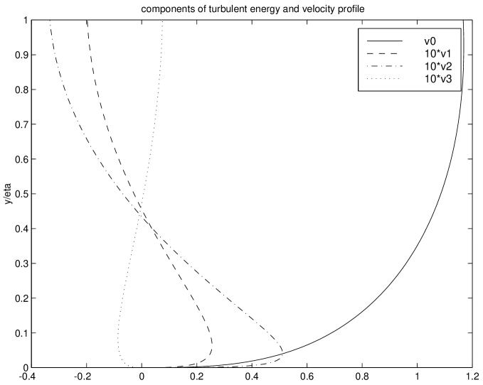
  Figure 2: the vertical structure functions for the turbulent energy density and horizontal velocity fields within the fluid as a function of the scaled vertical coordinate $\zeta=y/\eta$: ——–, $\upsilon_{0}(\zeta)$ (with $\gamma=1$); – – –, $10\times\upsilon_{1}(\zeta)$; –$\cdot$–$\cdot$–$\cdot$–, $10\times\upsilon_{2}(\zeta)$; $\cdot\cdot\cdot\cdot\cdot\cdot$, $10\times\upsilon_{3}(\zeta)$.

  Observe the cube-root structure in the vertical is modified to $\upsilon_{0}(\zeta)$. As shown in Figure 2, when $\gamma$ is set to $1$ to recover the original boundary conditions from (22), the cube-root dependence is maintained near the bed, but is effectively flattened near the fluid surface to closely approximate the absence of turbulent energy flux through the free surface. This correction is simultaneously determined with a corresponding decay term in the evolution equations, as seen below, due to the removal of the sustaining flux. We look even closer at the effects of modifying the free-surface boundary conditions in §§4.2.

  Also the effect of turbulent production, proportional to ${\bar{u}}^{2}$, through the velocity shear is largest near the bed; as seen in the shape of $\upsilon_{1}(\zeta)$ and $\upsilon_{2}(\zeta)$ this enhances turbulent energy $k$ near the bed.

  However, the natural turbulent dissipation within the fluid causes a relatively greater decay of turbulent energy near the bed as compared with the body of the fluid, as seen in $\upsilon_{3}(\zeta)$, and so counters this enhancement. Being proportional to $1/\tilde{\nu}$, this effect on the $k$-profile is greatest in weakly turbulent flows.

• The basic cube-root structure of the horizontal velocity is modified in exactly the same way and for the same reasons as for the basic turbulent energy $k$-profile.

  Modifications of the velocity profile due to the turbulent production and dissipation occur, but they occur primarily through the indirect effects of modifications to the turbulent diffusivity profile $\nu(\zeta)$. These are weak due to the subtractions in (29b).

• The corresponding vertical structure of the turbulent mixing coefficient $\nu$ is shown in Figure 3 where the five components are

  $$\nu_{0}(\zeta) = \frac{20}{9}\zeta^{2/3}-\frac{8}{9}\zeta^{2}\,,$$

  $$\nu_{1}(\zeta) = \frac{64}{135}\zeta^{2}-\frac{128}{135}\zeta^{4/3}+\frac{2944}{8505}\zeta^{2/3}\,,$$

  $$\nu_{2}(\zeta) = -\frac{32}{27}\zeta+\frac{4}{5}\zeta^{2/3}+\frac{8}{27}\zeta^{2}\,,$$

  $$\nu_{3}(\zeta) = \frac{57}{448}\zeta^{2/3}-\frac{3}{4}\zeta^{5/3}+\frac{9}{16}\zeta^{2}\,,$$

  $$\nu_{4}(\zeta) = \frac{33}{224}\zeta^{2/3}+\frac{9}{16}\zeta^{2}-\frac{3}{4}\zeta^{5/3}\,.$$

  

  Figure 3: the vertical structure functions for the turbulent mixing coefficient within the fluid as a function of the scaled vertical coordinate $\zeta=y/\eta$: ——– (right), $\nu_{0}(\zeta)$ (with $\gamma=1$); – – –, $10\times\nu_{1}(\zeta)$; –$\cdot$–$\cdot$–$\cdot$–, $10\times\nu_{2}(\zeta)$; $\cdot\cdot\cdot\cdot\cdot\cdot$, $10\times\nu_{3}(\zeta)$; ——– (left), $\nu_{4}(\zeta)$.

Simultaneously with the determination of the above fields, the solvability condition for the linear equations of the form (28) supplies terms in the asymptotic, low-dimensional evolution equations for the amplitudes of the four critical modes. Writing these in terms of physical variables we find, with errors ${\cal O}\left(\delta^{6}+\lambda^{3}+\gamma^{3},{\vartheta}\right)$:

$$\frac{\partial\eta}{\partial t} \sim 0\,,$$ (30a)

$$\frac{\partial{\bar{u}}}{\partial t} \sim -\frac{56\gamma\tilde{\nu}}{81\eta^{2}}{\bar{u}}-\frac{\lambda}{16}\left[C_{\epsilon 2}\sigma_{\epsilon}-\sigma_{k}\right]\frac{{\bar{\epsilon}}{\bar{u}}}{{\bar{k}}}+\frac{16}{81}\left[\frac{32}{45}C_{\epsilon 1}\sigma_{\epsilon}-\sigma_{k}\right]\frac{\tilde{\nu}{\bar{u}}^{3}}{\eta^{2}{\bar{k}}}\,,$$ (30b)

$$\frac{\partial{\bar{k}}}{\partial t} \sim -\lambda\left[\frac{7}{8}+\frac{C_{\epsilon 2}\sigma_{\epsilon}}{16\sigma_{k}}\right]{\bar{\epsilon}}-\frac{56\gamma\tilde{\nu}}{81\sigma_{k}\eta^{2}}{\bar{k}}+\frac{16}{243}\left[7+\frac{32C_{\epsilon 1}\sigma_{\epsilon}}{15\sigma_{k}}\right]\frac{\tilde{\nu}}{\eta^{2}}{\bar{u}}^{2}\,,$$ (30c)

$$\frac{\partial{\bar{\epsilon}}}{\partial t} \sim -\lambda\frac{9}{8}C_{\epsilon 2}\frac{{\bar{\epsilon}}^{2}}{{\bar{k}}}+\frac{256}{243}C_{\epsilon 1}\frac{\tilde{\nu}{\bar{\epsilon}}}{\eta^{2}{\bar{k}}}{\bar{u}}^{2}\,,$$ (30d)

where

$$\tilde{\nu}(x,t)=C_{\mu}\frac{{\bar{k}}^{2}}{{\bar{\epsilon}}}$$ (31)

is a measure of the local turbulent diffusivity. These form a crude approximation to the evolution equations for the four amplitudes of the model when there are no horizontal variations.

The two fifth-order evolution equations (30c–30d) summarise the turbulent production and decay processes. Setting the artificial parameters $\lambda=\gamma=1$ to approximate the dynamics of the original problem, observe: first, the natural decay of turbulent energy and dissipation in the body of the fluid; second, decay of turbulent energy with coefficient proportional to $\tilde{\nu}/\eta^{2}$ via turbulent mixing transporting energy to the bed; and third, the generation of turbulence energy and its dissipation through the shear in the vertical, proportional to $\tilde{\nu}{\bar{u}}^{2}/\eta^{2}$.

The horizontal velocity evolution (30b) similarly includes terms: $\tilde{\nu}{\bar{u}}/\eta^{2}$ which represents the effective drag of the bottom via turbulent mixing to the bed; and weak cubic, proportional to $\tilde{\nu}{\bar{u}}^{3}/(\eta^{2}{\bar{k}})$, and linear, proportional to ${{\bar{\epsilon}}{\bar{u}}}/{{\bar{k}}}$, modification of this drag through changes in the stress tensor in the momentum equations (note that the coefficients are the difference of two terms, and that with the usual values for the parameters (4) there is significant cancellation).

The free-surface stays horizontal, equation (30a), because there are no horizontal gradients until we look at order ${\vartheta}$ effects in a later subsection.

4.2 Convergence in the artificial parameters

One limitation on the accuracy of the above model is that even within the $k$-$\epsilon$ model of turbulence the coefficients are only approximate. This is due to both the modification of the free surface boundary conditions on $u$ and $k$ to (21–22); and the introduction of $\lambda$ in (20). Although setting $\gamma=1$ recovers the original boundary conditions (6–7) and $\lambda=1$ recovers the original $k$-$\epsilon$ model, there is no certainty that this will give a model which is a good approximation to the “true” system. In essence the coefficients in the model are multi-variable Taylor series in $\gamma$ and in $\lambda$. In this subsection we present evidence that these series converge for $\gamma=\lambda=1$ and so we can form a reasonable model.

Arbitrarily high order terms in the centre manifold expansion may be computed in principle. Our computer algebra program currently is limited by memory and time constraints to about 8th order in $\gamma$ and lower orders in other parameters. This is only attainable by the simplification of setting the $k$-$\epsilon$ parameters to the conventional numerical values in (4). By executing the reduce program and discarding terms ${\cal O}\left(\delta^{6},\gamma^{8},\lambda^{2},{\vartheta}\right)$, we discover more terms in the series in $\gamma$. Listed in Table 1 are the expansions of some of the coefficients appearing later in the models.

Table 1: terms in the series expansions in $\gamma$ of selected coefficients in the model for homogeneous turbulent decay. The last row is the sum of known terms at $\gamma=1$.

	in $\partial{\bar{u}}/\partial t$			in $\partial{\bar{k}}/\partial t$
	$-\tilde{\nu}{\bar{u}}/\eta^{2}$	$-\tilde{\nu}{\bar{u}}{\tilde{\lambda}}/\eta^{2}$	$\tilde{\nu}{\bar{u}}^{3}/\eta^{2}{\bar{k}}$	$\tilde{\nu}{\bar{u}}^{2}/\eta^{2}$	$-{\bar{\epsilon}}$
$1$	0	$+1.03889$	$+0.06542$	$+0.72385$	$+1.03100$
$\gamma$	$+0.69136$	$-0.86096$	$+0.01388$	$-0.13682$	$-0.05665$
$\gamma^{2}$	$+0.22783$	$+0.14923$	$-0.01564$	$-0.02193$	$+0.01602$
$\gamma^{3}$	$+0.07479$	$+0.02700$	$-0.00921$	$+0.00569$	$+0.00250$
$\gamma^{4}$	$+0.02448$	$+0.00462$	$-0.00333$	$+0.00814$	$+0.00027$
$\gamma^{5}$	$+0.00801$	$+0.00069$	$-0.00080$	$+0.00549$	$-0.00002$
$\gamma^{6}$	$+0.00262$	$+0.00006$	$-0.00003$	$+0.00300$	$-0.00003$
$\gamma^{7}$	$-0.00086$	$-0.00002$	$+0.00017$	$+0.00147$	$-0.00001$
$\sum$	$\phantom{+}1.02995$	$\phantom{+}0.35950$	$\phantom{+}0.05040$	$\phantom{+}0.58892$	$\phantom{+}0.99307$

Look down the columns in the table and see that the coefficients in each sequence generally decrease by at least a factor of two. This suggests that the radii of convergence of the series in $\gamma$ are roughly two or more. Thus simply evaluating the series’ at $\gamma=1$ is reasonably good—some are shown in the bottom line of the table.

The convergence in the parameter $\lambda$ is problematical because it seems to appear always in the combination $\lambda\eta^{2}{\bar{\epsilon}}/(\tilde{\nu}{\bar{k}})$, that is $\lambda\eta^{2}{\bar{\epsilon}}^{2}/{\bar{k}}^{3}$. Thus convergence depends upon the properties of the solution which is generally unknown beforehand. We suggest that truncating to linear terms in $\lambda$ forms an adequate approximation. It seems at least self-consistent to do this as later homogeneous solutions, namely (37–40), show a balance for the relatively small value $\eta^{2}{\bar{\epsilon}}^{2}/{\bar{k}}^{3}\approx 0.2$. Thus the nonlinear terms in $\lambda$ are generally expected to have a negligible influence in most flows of interest.

First, the series’ are summed for $\gamma=1$ as discussed in the previous subsection. Then introducing

$${\tilde{\lambda}}=\frac{\lambda\eta^{2}{\bar{\epsilon}}^{2}}{{\bar{k}}^{3}}=C_{\mu}\lambda\frac{\eta^{2}/\tilde{\nu}}{{\bar{k}}/{\bar{\epsilon}}}\propto\lambda\frac{\mbox{vertical mixing time}}{\mbox{turbulent eddy time}}\,,$$ (32)

for brevity we write the model of decay of homogeneous turbulent flow as follows, with errors ${\cal O}\left(\delta^{6},\lambda^{2},{\vartheta}\right)$,

$$\frac{\partial\eta}{\partial t} = 0\,,$$ (33a)

$$\frac{\partial{\bar{u}}}{\partial t} = -(1.030+0.359\,{\tilde{\lambda}})\frac{\tilde{\nu}{\bar{u}}}{\eta^{2}}+(0.0504-0.243\,{\tilde{\lambda}})\frac{\tilde{\nu}{\bar{u}}^{3}}{\eta^{2}{\bar{k}}}\,,$$ (33b)

$$\frac{\partial{\bar{k}}}{\partial t} = -(0.0927+0.993\,{\tilde{\lambda}})\frac{{\bar{k}}^{3}}{\eta^{2}{\bar{\epsilon}}}+(0.589+0.516\,{\tilde{\lambda}})\frac{\tilde{\nu}{\bar{u}}^{2}}{\eta^{2}}\,,$$ (33c)

$$\frac{\partial{\bar{\epsilon}}}{\partial t} = -2.101\,{\tilde{\lambda}}\frac{{\bar{k}}^{2}}{\eta^{2}}+(1.552-3.215\,{\tilde{\lambda}})\frac{\tilde{\nu}{\bar{\epsilon}}{\bar{u}}^{2}}{{\bar{k}}\eta^{2}}\,.$$ (33d)

Note that setting $\lambda=1$ to recover the original problem is just equivalent to using ${\tilde{\lambda}}={\eta^{2}{\bar{\epsilon}}^{2}}/{{\bar{k}}^{3}}$. Observe that the first terms on the right-hand sides of the above represent decay terms through, for example in the ${\bar{u}}$ and ${\bar{k}}$ equations, turbulent transport to the stream bed. The last terms in the ${\bar{k}}$ and ${\bar{\epsilon}}$ equations represent the production of turbulence through the velocity shear.

One feature of the model derived here is that it has no adjustable coefficients. All constants are derived from well known physical parameters and accepted constants of the $k$-$\epsilon$ equations. Despite its relative complexity, the model has been systematically derived and the constants which appear are well-defined. However, there are adjustable parameters, namely the order of truncation of the series expansions. The model (33), for example, contains just the low-order terms in expansions in $\delta$ and $\lambda$.

4.3 Dynamics of spatial structure

The leading order effect of horizontal gradients, such as due to a sloping free surface, is found by computing terms of order ${\vartheta}$ in the asymptotic expansions. We describe these in this subsection.

Dominantly, horizontal gradients affect the velocity and pressure fields. By computing terms to order $\delta^{3}{\vartheta}$ we find that the velocity fields (29a–29b) are modified to

$$v = -\zeta^{4/3}\eta\frac{\partial{{\bar{u}}}}{\partial{x}}+{\cal O}\left(\delta^{6}+\lambda^{3}+\gamma^{3}+{\vartheta}^{3}\right)\,,$$ (34a)

$$u = \cdots+3\upsilon_{3}(\zeta)\frac{g\eta^{2}}{\tilde{\nu}}\frac{\partial{\eta}}{\partial{x}}+{\cal O}\left(\delta^{6}+\lambda^{3}+\gamma^{3}+{\vartheta}^{3}\right)\,,$$ (34b)

where the $\cdots$ indicate the terms on the right-hand side of (29b), and where $\upsilon_{3}(\zeta)$ is drawn in Figure 2. The shape of $v$ is required by the continuity equation. The modification to $u$ asserts reasonably that at low levels of turbulence, large $1/\tilde{\nu}$, horizontal accelerations through decreasing depth, $\eta_{x}<0$, cause the fluid to respond with a flatter profile through a subtraction of $\upsilon_{3}(\zeta)$ from $\upsilon_{0}(\zeta)$ as seen in Figure 2.

The structure of the fields within the fluid rapidly become more complicated at higher order. We do not detail the fields any more.

By executing the computer algebra program and discarding generated terms ${\cal O}\left(\delta^{6},\gamma^{6},\lambda^{2},{\vartheta}^{2}\right)$, we discover first order effects of horizontal variations with sufficient terms in the series in $\gamma$ to sum them reliably for $\gamma=1$. We find the same production and decay terms identified in (33) and, in addition, extra terms in the horizontal gradients. Using the accepted values (4) for the constants of the $k$-$\epsilon$ equations, we obtain the following model with our best estimates of its coefficients:

$$\frac{\partial\eta}{\partial t} \sim -\frac{\partial(\eta{\bar{u}})}{\partial x}\,,$$ (35a)

$$\frac{\partial{\bar{u}}}{\partial t} \sim -(1.030+0.359\,{\tilde{\lambda}})\frac{\tilde{\nu}{\bar{u}}}{\eta^{2}}+(0.0504-0.243\,{\tilde{\lambda}})\frac{\tilde{\nu}{\bar{u}}^{3}}{\eta^{2}{\bar{k}}}$$ (35b)

$${}+\left[0.961-0.019\,{\tilde{\lambda}}-(0.019-0.087\,{\tilde{\lambda}})\frac{{\bar{u}}^{2}}{{\bar{k}}}\right]g\left(\theta-\frac{\partial\eta}{\partial x}\right)$$

$${}-(1.105+0.104\,{\tilde{\lambda}}){\bar{u}}\frac{\partial{\bar{u}}}{\partial x}-(0.032-0.056\,{\tilde{\lambda}})\frac{{\bar{u}}^{2}}{{\bar{k}}}\frac{\partial{\bar{k}}}{\partial x}$$

$$\quad{}+(0.025-0.041\,{\tilde{\lambda}})\frac{{\bar{u}}^{2}}{{\bar{\epsilon}}}\frac{\partial{\bar{\epsilon}}}{\partial x}\,,$$

$$\frac{\partial{\bar{k}}}{\partial t} \sim -0.0927\frac{{\bar{k}}^{3}}{\eta^{2}{\bar{\epsilon}}}-0.993\,{\bar{\epsilon}}+(0.589+0.516\,{\tilde{\lambda}})\frac{\tilde{\nu}{\bar{u}}^{2}}{\eta^{2}}$$ (35c)

$${}-(0.025+0.011\,{\tilde{\lambda}})g{\bar{u}}\left(\theta-\frac{\partial\eta}{\partial x}\right)$$

$${}-(1.106-0.065\,{\tilde{\lambda}}){\bar{u}}\frac{\partial{\bar{k}}}{\partial x}-(0.030+0.056\,{\tilde{\lambda}}){\bar{k}}\frac{\partial{\bar{u}}}{\partial x}$$

$$\quad{}+(0.025-0.060\,{\tilde{\lambda}})\frac{{\bar{u}}{\bar{k}}}{{\bar{\epsilon}}}\frac{\partial{\bar{\epsilon}}}{\partial x}\,,$$

$$\frac{\partial{\bar{\epsilon}}}{\partial t} \sim -2.101\frac{{\bar{\epsilon}}^{2}}{{\bar{k}}}+(1.552-3.215\,{\tilde{\lambda}})\frac{\tilde{\nu}{\bar{\epsilon}}{\bar{u}}^{2}}{{\bar{k}}\eta^{2}}$$ (35d)

$${}+\left(-0.006+0.562\,{\tilde{\lambda}}\right)g\frac{{\bar{u}}{\bar{\epsilon}}}{{\bar{k}}}\left(\theta-\frac{\partial\eta}{\partial x}\right)$$

$${}-0.173\,{\tilde{\lambda}}{\bar{\epsilon}}\frac{\partial{\bar{u}}}{\partial x}+0.533\,{\tilde{\lambda}}\frac{{\bar{\epsilon}}{\bar{u}}}{{\bar{k}}}\frac{\partial{\bar{k}}}{\partial x}-(1+0.735\,{\tilde{\lambda}}){\bar{u}}\frac{\partial{\bar{\epsilon}}}{\partial x}\,.$$

We expect that the coefficients in the above equations, when considered as a model of the $k$-$\epsilon$ equations given in Section 2, are accurate as shown. Except for the surface equation (35a), the first line in each equation is the same as in the horizontally homogeneous model (30); subsequent lines detail the additional terms needed to begin modelling long waves. A simpler version of the above model, obtained by omitting terms with small coefficients, is recorded in the Introduction as the model (1).

Equation (35a) is an exact statement of the conservation of water and is not modified by any higher-order effects. To $\delta^{3}{\vartheta}$, it may be written

$$\frac{\partial\eta}{\partial t}+h\frac{\partial{\bar{u}}}{\partial x}=0\,,$$ (36a)

which is a linear description of the conservation of water. Similarly, with $$\theta=0 \tilde{\nu}\approx 0 \delta^{3}{\vartheta}$$ and in very low levels of turbulence () the horizontal momentum equation (35b) may be written to as

$$\frac{\partial{\bar{u}}}{\partial t}=-0.961\,g\frac{\partial\eta}{\partial x}\,.$$ (36b)

This describes the horizontal acceleration due to slope of the fluid surface. These last two coupled equations form a standard description of linear wave dynamics except for one remarkable feature: the effect of gravity is reduced by the factor $0.961$. For example, this would predict that even low levels of turbulence reduces the phase speed of waves by about two percent. As in thin films of viscous fluid [39], the phenomenon is due to the response of the fluid, approximately $v_{0}(\zeta)$ shown in Figure 2, being at an angle to the forcing $1$ (either due to gravity or horizontal pressure gradients) when considered in the space of functions on $[0,\eta]$. Consequently, the forcing is less effective. Such a depression in phase speed may be observable in the propagation of long-waves on turbulent flow.

Returning to the order $\delta^{5}$ momentum equation (35b) we note several interesting effects.

• The first line contains the turbulent drag terms identified in the previous subsection.

• The second lines describe the effects of surface and bed slope. Within the square brackets:

  • the first term gives the depression of wave speed discussed above;

  • the second term very weakly enhances the phase speed correction in turbulent flow;

  • whereas it is difficult to ascribe one definite cause to the last term, coefficient modifications of the form ${\bar{u}}^{2}/{\bar{k}}$ are common in this model and reflect the relative importance of the turbulence on the mean flow.

• The third and fourth lines are dominated by the nonlinear advection term ${\bar{u}}{\bar{u}}_{x}$, with coefficient approximately $1.1$. This coefficient is larger than 1 because of the shear: the maximum $u(y)>{\bar{u}}$ advects itself faster than ${\bar{u}}$. This third line also shows small “cross-talk” effects in the advection through the ${\bar{u}}^{2}\left(\log{\bar{k}}\right)_{x}$ and ${\bar{u}}^{2}\left(\log{\bar{\epsilon}}\right)_{x}$ terms.

The dynamics of $k$ and $\epsilon$ averages are given by equations (35c–35d).

• The first lines of each equation are the same turbulent production and decay terms identified in the previous subsection.

• The next line in each equation may arise from the modification of the turbulent production through the change of the velocity profile, seen in (34b), due to horizontal acceleration.

• The remaining terms simply represent horizontal advection by the fluid velocity. Note that different properties are advected at different effective speeds as indicated by the different coefficients of the ${\bar{u}}\partial/\partial x$ terms: $1.1$ for ${\bar{u}}$ and ${\bar{k}}$, and $1$ for ${\bar{\epsilon}}$.

The model (1) reported in the introduction is a simplified version of (35). The solutions described in the next section show that the terms neglected from (35) in writing (1) are relatively small, contributing at most a few percent in the numerical balance of the terms, and so may be neglected at least for initial exploration.

5 Predictions of the new model

In this section we investigate some of the predictions the newly derived model (35) might make. We look at decaying turbulence, uniform flow on slopes, approximation to the St Venant equations, and a dam break simulation.

5.1 Decaying turbulence

Homogeneous turbulence decays algebraically. If there is no slope ($\theta=0$), no variations in $x$, no mean flow (${\bar{u}}=0$) and no surface waves ($\eta=\mbox{const}$), then it is consistent to seek solutions of the model (35) in the form ${\bar{k}}\propto t^{-2}$ and ${\bar{\epsilon}}\propto t^{-3}$. Substituting and solving for the constants of proportionality the model (35) predicts the turbulence decays according to

$${\bar{k}}\sim 8.97\,\eta^{2}t^{-2}\,,\quad{\bar{\epsilon}}\sim 12.8\,\eta^{2}t^{-3}\,,\quad\tilde{\nu}\sim 0.565\,\eta^{2}t^{-1}\,,\quad{\tilde{\lambda}}\sim 0.227\,.$$ (37)

for large time $t$. The turbulence ultimately decays with the balance ${\bar{\epsilon}}\sim 0.48\,{\bar{k}}^{3/2}/\eta$.

However, the transients towards this large time behaviour may be long. There are two regimes of interest characterised by large and small ${\tilde{\lambda}}$ compared to $0.227$ (recall from (32) that ${\tilde{\lambda}}$ is the ratio of the vertical mixing time to the turbulent eddy mixing time).

• For small ${\tilde{\lambda}}$, high turbulence ${\bar{k}}$ and low dissipation ${\bar{\epsilon}}$, the dissipation is roughly constant, actually

  $${\bar{\epsilon}}\approx\frac{1}{\sqrt{{\bar{\epsilon}}^{-2}_{\infty}+15.1/k^{3}}}\,,$$

  as the turbulence decays to (37) on a time scale of approximately $2(\eta^{2}/{\bar{\epsilon}})^{1/3}$.

• For large ${\tilde{\lambda}}$ the vertical mixing time is relatively rapid and the turbulence decays with a different power law for some time. We find that ${\bar{\epsilon}}\propto{\bar{k}}^{2.11}$ which is only a little different from (37). The rate of decay towards (37) is relatively slow,

  $$({\bar{k}},{\bar{\epsilon}})\approx A\left(t^{-0.90},0.90\,t^{-1.90}\right)\,,$$

  and forms a long lasting transient.

The above results are for stationary water. Instead, if the water is moving with uniform velocity on a horizontal bed then the characteristics of the decaying bulk motion and turbulence are different in detail. We seek solutions of the model (35) in the form ${\bar{k}}\propto t^{-2}$ and ${\bar{\epsilon}}\propto t^{-3}$, as before, but now with ${\bar{u}}\propto t^{-1}$. Substituting and solving for the constants of proportionality the model (35) may be rewritten as a generalised eigenvalue problem for ${\tilde{\lambda}}$. It is then straightforward to determine the only positive solution is

$${\bar{u}}\sim 5.52\,\eta t^{-1}\,,\quad{\bar{k}}\sim 20.4\,\eta^{2}t^{-2}\,,\quad{\bar{\epsilon}}\sim 41.1\,\eta^{2}t^{-3}\,,\quad$$

$$\tilde{\nu}\sim 0.91\,\eta^{2}t^{-1}\,,\quad{\tilde{\lambda}}\sim 0.199\,.$$ (38)

Numerical solutions show that there are long lasting transients of a similar nature to those mentioned above for stationary water. We do not elaborate further as this class of solutions are less likely to be of interest in applications.

5.2 Turbulence in balance with fluid flow

Water flowing down a slope generates turbulence that provides the drag to balance the gravitational forcing. Let the downward bed slope be $\theta\neq 0$, but as in the previous subsection assume are no variations in $x$, that is, just a mean flow (${\bar{u}}\neq 0$) with no surface waves ($\eta=\mbox{const}$). Then it is consistent to seek solutions of the model (35) in the form ${\bar{u}}\propto\eta^{1/2}\theta^{3/2}$, ${\bar{k}}\propto\eta\theta$ and ${\bar{\epsilon}}\propto\eta^{1/2}\theta^{3/2}$. Substituting and solving for the constants of proportionality leads to a nonlinearly perturbed eigenvalue problem for ${\tilde{\lambda}}$ which is solved iteratively to give

$${\bar{u}}\approx 3.16\,\eta^{1/2}(g\theta)^{1/2}\,,\quad{\bar{k}}\approx 1.95\,\eta g\theta\,,\quad{\bar{\epsilon}}\approx 1.27\,\eta^{1/2}(g\theta)^{3/2}\,,\quad$$

$$\tilde{\nu}\approx 0.270\,\eta^{3/2}(g\theta)^{1/2}\,,\quad{\tilde{\lambda}}\approx 0.217\,.$$ (39)

We expect this flow to be established on a time scale of the vertical mixing which is

$$T_{\mbox{\scriptsize mix}}=\frac{\eta^{2}}{\tilde{\nu}}\approx 4\sqrt{\frac{\eta}{g\theta}}\,.$$

Another interesting balance occurs when we assume that the production of turbulence parameters, ${\bar{k}}$ and ${\bar{\epsilon}}$, equals their dissipation through natural dissipation and bed drag. This leads to a reduced model in the form of St Venant’s equation used in open channel flow. Assume that at all times the production and dissipation of ${\bar{k}}$ and ${\bar{\epsilon}}$ in the first lines on the right-hand sides of (35c) and (35d). That is, assume the bed slope is small enough and the flow is evolving slowly enough that spatial and temporal gradients are negligible. Then seek a balance with ${\bar{k}}\propto{\bar{u}}^{2}$ and ${\bar{\epsilon}}\propto{\bar{u}}^{3}$ to find

$${\bar{k}}\approx 0.224\,{\bar{u}}^{2}\,,\quad{\bar{\epsilon}}\approx 0.0453\,{\bar{u}}^{3}/\eta\,,\quad\tilde{\nu}\approx 0.0992\,\eta{\bar{u}}\,,\quad{\tilde{\lambda}}\approx 0.184\,.$$ (40)

With this balance the momentum equation (35b) becomes

$$\frac{\partial{\bar{u}}}{\partial t}=-0.111\frac{{\bar{u}}^{2}}{\eta}+0.94\,g\left(\theta-\frac{\partial\eta}{\partial x}\right)-1.12\,{\bar{u}}\frac{\partial{\bar{u}}}{\partial x}-0.018\frac{{\bar{u}}^{2}}{\eta}\frac{\partial\eta}{\partial x}\,,$$ (41)

which has exactly the same form as St Venant’s equation for open channel flow except for the small term ${\bar{u}}^{2}\eta_{x}/\eta$. The three significant coefficients are worthy of comment: the self-advection coefficient of $1.12$ accounts for the vertical nonuniformity of the velocity profile with mean ${\bar{u}}$; the influence of gravity is reduced to $0.94\,g$ because, as explained earlier for (36b), the response of the fluid flow is not constant in the vertical so some of gravitational forcing is not used; and lastly the bed drag ${\bar{u}}^{2}/\eta$ has coefficient $0.111$ which is larger than typical values. However, note that such drag coefficients have to vary depending upon the roughness of the channel bottom as often expressed by different roughness coefficients in Manning’s law [6, p246,e.g.] or [22, p137,e.g.]. We surmise that the flows we describe with model (35) have strong mixing in the vertical due to strong turbulence generated by a rough channel bed or other extremely turbulent flows such as breaking waves or dam spillways.

5.3 Simulate a dam breaking

One of the canonical flows of shallow water occurs after a dam breaks. Here we simulate such a flow and resolve the water slumping downstream and becoming extremely turbulent as it does so. For simplicity we use the model (1) reported in the introduction.

Imagine a dam at $x=0$ initially holding back water of non-dimensional depth $\eta=1$. At time $t=0$ the dam breaks and releases the water to rush downstream. To avoid overly poor conditioning in the numerics we let the water in front of the dam be of depth $\eta=0.2$ (all quantities will no be non-dimensional so that in effect $g=1$). Also to smooth the initial few time steps we actually set $\eta$ to a tanh profile that smoothly varied between these extremes such that the water slope was a maximum of $2$ (rather large under the slowly varying assumption) at the dam. The water is assumed initially quiescent, ${\bar{u}}=0$ throughout, and has a low level of turbulence, somewhat arbitrarily chosen to be ${\bar{k}}=0.001$. Turbulent dissipation is initially set to ${\tilde{\lambda}}=0.227$ so that the balance of decaying turbulence (37) holds throughout.

The model (1) is simply discretised on a regular grid in space-time with a time step of $\Delta t=1/10$ and space step of $\Delta x=1/6$. The equations are discretised using a six point stencil, 3 wide in space and 2 in time, and using second order accurate centred differencing in both space and time. This leads to a sparse set of nonlinear implicit equations for the variables at the new time given their values at any given time. The nonlinear equations are solved by a few Newton’s iterations requiring that the maximum norm of the residuals be less than $10^{-4}$. The model (1) is purely hyperbolic, so a small amount of spatial diffusion is incorporated to help stabilise the simulation. It was physically appealing to incorporate the turbulent diffusion $(\tilde{\nu}{\bar{u}}_{x})_{x}$ into the ${\bar{u}}$ equation and similarly for for ${\bar{k}}$ and ${\bar{\epsilon}}$. Such diffusion made hardly any difference to the simulations as a whole yet usefully avoided the generation of unphysical and ruinous spikes in the numerical solution. The domain of simulation extended from six dam heights to the left behind the dam to six dam heights downstream. We integrated for over a time $t=7$ which is long enough for the disturbance to reach the ends of the computational domain (linear waves on the dammed water having speed 1).

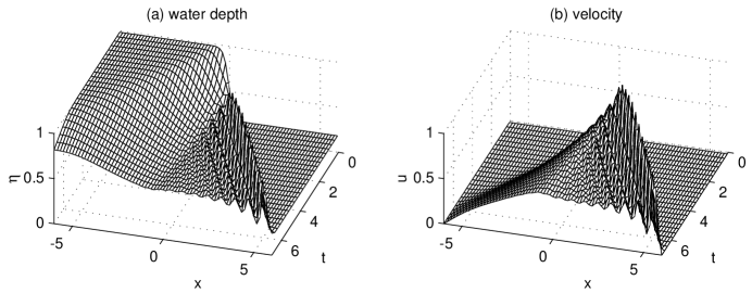
Figure 4: simulation of dam breaking showing (a) the water depth $\eta$ and (b) the mean downstream velocity ${\bar{u}}$. Observe the formation of a bore with superposed waves.

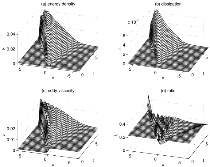
Figure 5: simulation of dam breaking showing the time evolution of the turbulence parameters (note the view point is rotated from Figure 4): (a) the turbulent energy density ${\bar{k}}$ is highest just a little behind the bore and then tails away; (b) the turbulent dissipation ${\bar{\epsilon}}$ behaves similarly; (c) the turbulent eddy viscosity $\tilde{\nu}$ is greatest at the front of the bore; and (d) the parameter ${\tilde{\lambda}}$, apart from a peak at he front of the bore, is generally depressed from the decaying balance value of $0.227$.

The results of this simulation are shown in Figures 4 and 5. Observe that when the dam breaks, the water slumps down and rushes downstream in a turbulent bore. The bore appears undular but may be evolving towards a series of solitary waves—they cannot be differentiated on this time-scale. The turbulent structure shown in Figure 5 has interesting features. Apparently the energy density peaks a little behind the bore, then decays approximately linearly with distance. It appears that up to time $t=7$ the generation of turbulence is still significantly greater than its decay as the peak is still growing. The turbulent dissipation and eddy viscosity behave similarly, though the eddy viscosity appears to peak much closer to the front of the turbulent bore. The parameter ${\tilde{\lambda}}$ plotted in Figure 5(d) reaffirms that relatively small values appear relevant to flows of interest. The peak of ${\tilde{\lambda}}$ at the front of the bore predicts that there is a lot of vertical mixing at the front, but less so behind the bore where ${\tilde{\lambda}}$ is smaller. All of the above seem physically reasonable.

This model that we have derived and solved in some cases of interest explicitly accounts for the spatio-temporal variations of the intensity and broad nature of the turbulence underlying the flow of shallow water.

Acknowledgement

This research was supported by a grant from the University of Southern Queensland, by the Australian Research Council, and by the Volkswagen Foundation, Germany, I/69449.

Appendix A Comments on theory in this application

This appendix addresses the connection to the rigorous theory of centre manifolds in this application.

It must be emphasised that throughout this paper we describe the application of centre manifold techniques and not the application of the rigorous centre manifold theory. There are two main reasons for this which we elaborate on below.

Firstly, here we construct an infinite dimensional centre manifold. At each point in $x$ there are four degrees of freedom, parametrised by $\eta$, $\bar{u}$, $\bar{k}$ and $\bar{\epsilon}$; but there are an infinitude of $x$ positions and so there is an infinite number of degrees of freedom in the mathematical model. However, there is currently very little theory on infinite dimensional centre manifolds appearing via slowly-varying approximations [15, e.g.], and what there is does not rigorously apply here, nor does it apply to many other physically interesting models such as dispersion in pipes [29], laminar long-wave, thin-film flows [39], and the dynamics in flow reactors [5]. Instead we use the formal techniques of constructing complete low-dimensional models [10, 34, 35, 36, 37], techniques suggested and developed by standard applications of the theory. We expect that eventually theory will be developed which supports the application of centre manifold concepts to slowly-varying approximations.

But there is a second obstacle to supporting this model with theory. In standard applications of centre manifold theory the nonlinear terms in the original problem are required to be smooth in the neighbourhood of the equilibrium under consideration (here the origin, a state of no flow and no turbulence). However, here many nonlinear terms are definitely not smooth; for example, turbulent dispersion terms such as $\frac{\partial{~{}}}{\partial{x}}\left(C_{\mu}\frac{k^{2}}{\epsilon}\frac{\partial{u}}{\partial{x}}\right)$ and interaction terms such as $C_{\epsilon 2}{\epsilon^{2}\over k}$ are unbounded as $(u,k,\epsilon)\to\mbox{\boldmath$0$}$. In rigorous applications of centre manifold theory, one may choose the various critical modes and parameters to have any set of relative orders of magnitude. The resulting asymptotic expressions are the same [34], it is only the sequence in which the terms appear that changes with a change in relative orders of magnitude. Indeed, this reflects a very desirable property of a modelling procedure, namely that the results are essentially independent of arbitrary human-made assumptions (such as order of magnitude) in the analysis. However, in this application the highly nonsmooth nature of the original equations means that in order to apply the centre manifold techniques we need to choose carefully the various orders of magnitudes of the variables and parameters, via (24). The aim, as in all asymptotic analyses, is to obtain a tractable and physically relevant leading order problem. The techniques of centre manifold theory are then applied, it is just that the current centre manifold theorems cannot give rigorous justification.

Notwithstanding these theoretical limitations we consider the systematic techniques are applicable because of the attractivity of the manifold of equilibria, ${\cal M}_{0}$, of the linear operator ${\cal L}$. In the spirit of centre manifold theory, we claim that the “small nonlinear” terms on the right-hand side of (20) just perturb the shape of ${\cal M}_{0}$ to a nearby manifold ${\cal M}$ and perturb the evolution thereon. Thus our last task, and the one fulfilled in this Appendix, is to prove the exponential decay to ${\cal M}_{0}$.

Linearising the $k$-$\epsilon$ equations (20) about ${\cal M}_{0}$

$$(p_{0},\mbox{\boldmath$u$}_{0})=\left(g(h-y),{\textstyle\frac{4}{3}{\left(\frac{y}{h}\right)^{1/3}}}U(x,t),0,H(x,t),{\textstyle\frac{4}{3}{\left(\frac{y}{h}\right)^{1/3}}}K(x,t),E(x,t)\right)\,,$$ (42)

we obtain $(0,\partial\mbox{\boldmath$u$}/\partial t)={\cal L}(p,\mbox{\boldmath$u$})$ where the linear operator ${\cal L}$ is

$$\left[\matrix{0&0&\frac{\partial{\cdot}}{\partial{y}}&0&0&0\cr 0&\frac{\partial{~{}}}{\partial{y}}\left(\nu_{0}\frac{\partial{\cdot}}{\partial{y}}\right)&0&0&C_{\mu}\frac{\partial{~{}}}{\partial{y}}\left(\frac{\partial{u_{0}}}{\partial{y}}{2k_{0}\over\epsilon_{0}}\cdot\right)&-C_{\mu}\frac{\partial{~{}}}{\partial{y}}\left(\frac{\partial{u_{0}}}{\partial{y}}{k_{0}^{2}\over\epsilon_{0}^{2}}\cdot\right)\cr-\frac{\partial{\cdot}}{\partial{y}}&0&2\frac{\partial{~{}}}{\partial{y}}\left(\nu_{0}\frac{\partial{\cdot}}{\partial{y}}\right)&0&-\frac{2}{3}\frac{\partial{\cdot}}{\partial{y}}&0\cr 0&0&0&0&0&0\cr 0&0&0&0&{C_{\mu}\over\sigma_{k}}\frac{\partial{~{}}}{\partial{y}}\left({k_{0}^{2}\over\epsilon_{0}}\frac{\partial{\cdot}}{\partial{y}}+{2k_{0}\over\epsilon_{0}}\frac{\partial{k_{0}}}{\partial{y}}\cdot\right)&-\frac{C_{\mu}}{\sigma_{k}}\frac{\partial{~{}}}{\partial{y}}\left(\frac{\partial{k_{0}}}{\partial{y}}{k_{0}^{2}\over\epsilon_{0}^{2}}\cdot\right)\cr 0&0&0&0&0&{C_{\mu}\over\sigma_{\epsilon}}\frac{\partial{~{}}}{\partial{y}}\left({k_{0}^{2}\over\epsilon_{0}}\frac{\partial{\cdot}}{\partial{y}}\right)}\right],$$

subject to boundary conditions

$$p+\frac{2}{3}k = 0\quad\mbox{on $y=h$\,,}$$ (43)

$$u = 0\quad\mbox{on $y=0$\,,}$$ (44)

$$\frac{\partial u}{\partial y}-\frac{u}{3h} = 0\quad\mbox{on $y=h$\,,}$$ (45)

$$v = 0\quad\mbox{on $y=0$\,,}$$ (46)

$$k = 0\quad\mbox{on $y=0$\,,}$$ (47)

$$\frac{\partial k}{\partial y}-\frac{k}{3h} = 0\quad\mbox{on $y=h$\,,}$$ (48)

$$y^{2/3}\frac{\partial\epsilon}{\partial y} \to 0\quad\mbox{as $y\to 0$\,,}$$ (49)

$$\frac{\partial\epsilon}{\partial y} = 0\quad\mbox{on $y=h$\,.}$$ (50)

We seek solutions proportional to $\exp(\lambda t)$. The first thing to note is that we address a generalised eigen-problem

$${\cal L}\left[\begin{array}[]{c}p_{0}\\ \mbox{\boldmath$u$}\end{array}\right]=\left[\begin{array}[]{c}0\\ \lambda\mbox{\boldmath$u$}\end{array}\right]$$

as the first row of ${\cal L}$ comes from the continuity equation.

Thus the first row, with the boundary condition (46), gives $v=0$ for any eigenvalue $\lambda$. Furthermore, the third row, from the vertical momentum equation with the pressure boundary condition (43), then gives that $p=-\frac{2}{3}k$ for any $\lambda$. These considerations give no constraint on the eigenvalue $\lambda$. Ignoring the $p$ and $v$ components of the eigen-problem then lead to a standard eigen-problem; one where the operator is in block, upper-triangular form. Thus consider the components in turn, starting from the last, and we show that all eigenvalues must be non-positive and thus ${\cal M}_{0}$ is attractive.

• For any eigen-function $u$, if turbulent dissipation $\epsilon\neq 0$, then

  $$\frac{h^{4/3}}{T\sigma_{\epsilon}}\frac{\partial{~{}}}{\partial{y}}\left(y^{2/3}\frac{\partial{\epsilon}}{\partial{y}}\right) = \lambda\epsilon\,,$$ (51)

  where

  $$T=\frac{9h^{2}}{16\tilde{\nu}}\,,$$

  is the time-scale of cross-depth turbulent diffusion. Multiplying (51) by $\epsilon$, $\int_{0}^{h}\cdots dy$, and integrating by parts we deduce

  $$\lambda=-\frac{h^{4/3}}{T\sigma_{\epsilon}}\frac{\int_{0}^{h}y^{2/3}\left(\frac{\partial{\epsilon}}{\partial{y}}\right)^{2}dy}{\int_{0}^{h}\epsilon^{2}dy}\leq 0\,,$$

  provided that the boundary conditions (50) (assuming $\epsilon\not\to\infty$ for $y\to h$) and

  $$\epsilon\frac{\partial\epsilon}{\partial y}=o\left(y^{-2/3}\right)\quad\mbox{as $y\to 0$,}$$ (52)

  are satisfied. The equality $\lambda=0$ holds if and only if $\frac{\partial\epsilon}{\partial y}\equiv 0$, which leads to

  $$\epsilon=E(x,t)\,,$$

  a function independent of $y$. Since equation (51) indicates nontrivial solutions near $y=0$ are of the form $\epsilon\sim A+By^{1/3}$, then the condition (52) is effectively equivalent to (49).

  Further, apply Sturm-Liouville theory to (51) under boundary conditions (50) and (49). Changing the vertical variable from $y=hz^{3}$ to $z$, the eigenvalue problem becomes

  $$\frac{\partial{{}^{2}\epsilon}}{\partial{z^{2}}}=9T\sigma_{\epsilon}\lambda z^{2}\epsilon\,,$$

  (a form of Bessel’s equation [1, Eq.9.1.51]) with the following normal separate boundary conditions

  $$\frac{\partial\epsilon}{\partial z}=0\quad\mbox{on $y=0$ and $y=h$.}$$

  Applying standard Sturm-Liouville theory, see for example Birkhoff & Rota [8, pp. 296] or Hartman [19, pp. 337ff], we see that the eigenvalues are discrete and must tend to infinity,

  $$0=\lambda_{1}>\lambda_{2}>\cdots\to-\infty\,.$$

  Thus, linearly, solutions in the neighbourhood of the manifold ${\cal M}_{0}$ are attracted exponentially quickly to it (at a rate at least as fast as $\exp(\lambda_{2}t)$).

  Sturm-Liouville theory may be also applied directly for the $u$ and $k$ components to show that any eigenvalues associated primarily with them are discrete. We do not record the details in the following.

• Similarly, for any eigen-function $u$, if turbulent dissipation $\epsilon=0$ but the turbulent energy $k\neq 0$, then

  $$\frac{h^{4/3}}{T\sigma_{k}}\frac{\partial{~{}}}{\partial{y}}\left(y^{2/3}\frac{\partial{k}}{\partial{y}}+\frac{2k}{3y^{1/3}}\right) = \lambda k\,.$$ (53)

  Multiplying this by $y^{2/3}$ we rewrite it as

  $$\frac{h^{4/3}}{T\sigma_{k}}y^{-1/3}\frac{\partial{~{}}}{\partial{y}}\left[y^{2}\frac{\partial{~{}}}{\partial{y}}\left(y^{-1/3}k\right)\right]=\lambda y^{2/3}k\,.$$

  Multiplying by $k$, $\int_{0}^{h}\cdots dy$ and integrating by parts we deduce

  $$\lambda=-\frac{h^{4/3}}{T\sigma_{k}}\frac{\int_{0}^{h}y^{2}\left[\frac{\partial{~{}}}{\partial{y}}\left(y^{-1/3}k\right)\right]^{2}dy}{\int_{0}^{h}y^{2/3}k^{2}dy}\leq 0\,,$$

  provided (48) and

  $$k=o\left(y^{1/12}\right)\quad\mbox{as $y\to 0$\,,}$$ (54)

  are satisfied. The equality $\lambda=0$ holds here if and only if $\frac{\partial{~{}}}{\partial{y}}\left(y^{-1/3}k\right)\equiv 0$, which together with boundary condition (47) implies

  $$k=K(x,t){\textstyle\frac{4}{3}{\left(\frac{y}{h}\right)^{1/3}}}$$

  with a function $K(x,t)$ independent of $y$. Since the indicial equation of (53) indicates nontrivial solutions near $y=0$ are of the form $k\sim Ay^{-2/3}+By^{1/3}$, then the boundary condition (54) is equivalent to (47).

• The only possible eigenvalue associated with non-zero $\eta$ is $0$.

• Lastly, for any eigen-function $u$, if $\epsilon=k=\eta=0$ but the horizontal velocity $u\neq 0$, then

  $$\frac{h^{4/3}}{T}\frac{\partial{~{}}}{\partial{y}}\left(y^{2/3}\frac{\partial{u}}{\partial{y}}\right) = \lambda u\,,$$ (55)

  and we rewrite this as

  $$\frac{h^{4/3}}{T}y^{-1/3}\frac{\partial{~{}}}{\partial{y}}\left[y^{4/3}\frac{\partial{~{}}}{\partial{y}}\left(y^{-1/3}u\right)\right]=\lambda u\,.$$

  Multiplying by $u$, $\int_{0}^{h}\cdots dy$ and integrating by parts we deduce

  $$\lambda=-\frac{h^{4/3}}{T}\frac{\int_{0}^{h}y^{4/3}\left[\frac{\partial{~{}}}{\partial{y}}\left(y^{-1/3}u\right)\right]^{2}dy}{\int_{0}^{h}u^{2}dy}\leq 0\,,$$

  provided (45) and

  $$u=o\left(y^{1/6}\right)\quad\mbox{as $y\to 0$\,,}$$ (56)

  are satisfied. Similarly to the $\epsilon$ and $k$ equations, the equality $\lambda=0$ holds here if and only if $\frac{\partial{~{}}}{\partial{y}}\left(y^{-1/3}u\right)\equiv 0$. This and the boundary condition (47) yields a unique solution

  $$u=U(x,t){\textstyle\frac{4}{3}{\left(\frac{y}{h}\right)^{1/3}}}$$

  with $U(x,t)$ independent of $y$. Since the indicial equation of (55) indicates nontrivial solutions near $y=0$ are of the form $u\sim A+By^{1/3}$, then the boundary condition (56) is effectively equivalent to (44).

We have proven: if the boundary conditions (43–50) are satisfied, then, except for the four-fold eigenvalue zero whose eigenfunctions span ${\cal M}_{0}$, the eigenvalues of ${\cal L}$ are negative and bounded away from $0$. Thus we expect the manifold (42) is locally attractive. Further, the time-scale of this attraction is the cross-depth turbulent diffusion time-scale $T$.

Appendix B Computer algebra

Here we list the reduce computer algebra program used to derive the long-wave models of turbulent flow.

The algorithm is the iterative algorithm described in [41, 43] adapted to this difficult asymptotic problem. The program refines the description of the centre manifold and the evolution thereon until the residual of the governing differential equations are driven to zero, to some asymptotic error. The key to the correctness of the results is then in the correct coding of the residuals—see inside the iterative loop.

Note that because the thickness of the film is continuously varying in space and time, and because of the cube-root structure in the vertical, it is convenient to work with equations in terms of a scaled vertical coordinate $z=\sqrt[3]{y/\eta}$ so that the free surface of the film is always $z=1$. However, the turbulence equations are not explicitly rewritten in this new coordinate because the computer handles all the necessary details of the transformation.

COMMENT Constructs a model of turbulent 2D flow of shallow water flow
on a flat slope based on the k-epsilon turbulence dynamical equations.
Calculates the centre manifold & reduced dynamic system on it for the
k-\epsilon model with the following boundary conditions for u, v, p, k
and \epsilon: u=v=k=deps/dy=0 at y=0, dk/dn=deps/dn=0 on y=eta. Fiddle
the free-surface BC to linearly force u & k at the surface. This gives
roughly cube-root profile in the vertical structure of u & k, whereas
eps is roughly constant.  Write results in terms of z=(y/eta)^(1/3).
Here scale derivatives as ddx*del for better control.
Created 11/11/94, last modified 8/6/99;
% improve output appearance
on div; off allfac; on list; on revpri;
factor es,ks,eta,us,del,ddx,df,g;
% maximum order of calculation in del: linear=3; non-trivial=5
o:=5;
% truncate in parameters: d/dx; BC kludge; k-eps fudge
let { ddx^2=>0, gamm^4=>0, lamb^2=>0};
% let ddx=>0; gamm:=del^2*gam; lamb:=lam*del^2; % for initial results
cgam:=(1-gamm*1/2); % equivalent to an Euler transform of gam series
theta:=del^3*ddx*thet;
% turbulence constants---remove to get general formulae
C_m:=9/100; C_e2:=192/100; C_e1:=144/100; s_k:=1; s_e:=13/10;
% FOR ALL q SUCH THAT  q>o LET del^q=0$
procedure ignore_order_gt(o); begin
IF o=3 THEN LET del^4=0;
IF o=4 THEN LET del^5=0;
IF o=5 THEN LET del^6=0;
IF o=6 THEN LET del^7=0;
IF o=7 THEN LET del^8=0;
IF o=8 THEN LET del^9=0;
IF o=9 THEN LET del^10=0;
IF o=10 THEN LET del^11=0;
IF o>=11 THEN LET del^12=0;
end;
% amplitudes and their dependences  ( eta=h+hs )
depend us,x,t;
depend ks,x,t;
depend es,x,t;
depend hs,x,t;
let {df(us,t) => gu,
     df(hs,t) => gh,
     df(ks,t) => gk,
     df(es,t) => ge
     };
% since z=(y/eta)^1/3 we need the following for d/dx, d/dt & d/dy
etax:=del^2*del*ddx*df(hs,x);
procedure dfdx(a);
begin scalar aa,bb;
      aa:=a*del^3*ddx; bb:=a*del*ddx;
      return df(bb,x) +( df(aa,eta) -z/3/eta*df(aa,z) )*df(hs,x);
end;
procedure dfdt(a);
begin scalar aa,ugh;
      aa:=a*del^2*del*ddx; ugh:=if gh=0 then 0 else gh/(del*ddx);
      return df(a,t) +( df(aa,eta) -z/3/eta*df(aa,z) )*ugh ;
end;
depend z,y;
let df(z,y) => 1/(3*eta*z^2);
fs:={z=1}$
% procedures to solve for cross-stream structures
operator iav;  linear iav;
operator ise;  linear ise;
operator isk;  linear isk;
operator isu;  linear isu;
operator isp;  linear isp;
operator isv;  linear isv;
let {iav(z^~p,z) => 1/(p+1)
    ,ise(z^~p,z) => ( z^(p+2) -3/(p+5) )/(p+1)/(p+2)
    ,isk(z^~p,z) => ( z^(p+2) -z*4/(p+5) )/(p+1)/(p+4)
    ,isu(z^~p,z) => ( z^(p+2) -z*4/(p+5) )/(p+1)/(p+2)
    ,isp(z^~p,z) => ( z^(p+1) -1 )/(p+1)
    ,isv(z^~p,z) => ( z^(p+1) )/(p+1)
    ,iav(z,z) => 1/2
    ,ise(z,z) => ( z^3 -1/2 )/6
    ,isk(z,z) => ( z^3 -z*2/3 )/10
    ,isu(z,z) => ( z^3 -z*2/3 )/6
    ,isp(z,z) => ( z^2 -1 )/2
    ,isv(z,z) => ( z^2 )/2
    ,iav(1,z) => 1
    ,ise(1,z) => ( z^2 -3/5 )/2
    ,isk(1,z) => ( z^2 -z*4/5 )/4
    ,isu(1,z) => ( z^2 -z*4/5 )/2
    ,isp(1,z) => ( z -1 )
    ,isv(1,z) => ( z )
    };
procedure mean(a);   3*iav(a*z^2,z);
procedure solv_e(a); 9/16*9*eta^2*s_e/anu*ise(z^2*a,z);
procedure solv_k(a); 9/16*9*eta^2*s_k/anu*isk(z^2*a,z);
procedure solv_u(a); 9/16*9*eta^2/anu*isu(z^2*a,z);
procedure solv_p(a); 3*eta*isp(z^2*a,z);
procedure solv_v(a); 3*eta*isv(z^2*a,z);
%%%%%%%%%%%%%%%%%%%%%%%%%%%%%%%%%%%%%%%%%%%%%%%%%%%%%%%%%%%%%%%%%%%%%%
% initial approximation for the iteration
cbrt:=(4/3)*z$
vu:=del^2*cbrt*us;
vv:=0;
vp:=g*eta*(1-z^3) +del^2*8/9*ks*(-z);
vk:=del^2*cbrt*ks;
ve:=del^3*es;
vnu:=c_m*vk^2/ve;;
vmu:=c_e2*ve^2/vk;
vph:=0;
gu:=0;
gh:=0;
gk:=0;
ge:=0;
%%%%%%%%%%%%%%%%%%%%%%%%%%%%%%%%%%%%%%%%%%%%%%%%%%%%%%%%%%%%%%%%%%%%%%
% iterate
anu:=c_m*ks^2/es$ % scaled typical diffusion
sinth:=theta-theta^3/6+theta^5/120-theta^7/5040$
costh:=1-theta^2/2+theta^4/24-theta^6/720$
repeat begin
write "
 NEXT ITERATION
----------------";
begin scalar Eqc;
ignore_order_gt(o);
% continuity equation for v
Eqc:=dfdx(vu)+df(vv,y);
ok:=if Eqc=0 then 1 else 0;
vv:=vv-solv_v(Eqc);
end;
% kinematic equation for eta
gh:=SUB(fs, vv-vu*etax )/del^2;
% mu equation for mu of sufficient order
begin scalar Eqmu;
ignore_order_gt(o+3);
Eqmu:=(vmu*vk-C_e2*ve^2)$
ok:=if ok and(Eqmu=0) then 1 else 0;
vmu:=vmu-Eqmu/(del^2*cbrt*ks);
end;
% ph production equation of order m-1
begin scalar Eqph;
ignore_order_gt(o-1);
Eqph:=(vph-(df(vu,y)+dfdx(vv))^2-2*df(vv,y)^2-2*dfdx(vu)^2)$
ok:=if ok and(Eqph=0) then 1 else 0;
vph:=vph-Eqph;
end;
% epsilon equation of order m+1 & BC of order m
begin scalar Eqeps,BCe0,BCeh,gep;
ignore_order_gt(o+1);
Eqeps:= -dfdt(ve) -lamb*vmu +C_e1*(del*es/ks)*vnu*vph
       +1/s_e*df(vnu*df(ve,y),y) -vu*dfdx(ve)-vv*df(ve,y)
       +1/s_e*dfdx(vnu*dfdx(ve))$
BCe0:=del*sub(z=0,z^2*df(ve,y))$
BCeh:=del*sub(fs, df(ve,y)-etax*dfdx(ve) )$
ok:=if ok and(Eqeps=0)and(BCe0=0)and(BCeh=0) then 1 else 0;
gep:=+mean(Eqeps)-160/117*anu/eta*BCeh;
ve:=ve-solv_e( Eqeps-gep )/del
      +27*eta*es/(32*ks^2*C_m*del)*BCe0*((1-z)^2-1/10);
ge:=ge+gep/del^3;
end;
% nu equation of order m+1
begin scalar Eqnu;
ignore_order_gt(o+1);
Eqnu:=vnu*ve-C_m*vk^2$
vnu:=vnu-Eqnu/(del^3*es);
end;
% k equation & (BC of order m-1)
begin scalar Eqk,BCk0,BCkh,gkp;
ignore_order_gt(o);
Eqk:= -dfdt(vk) -lamb*ve +vnu*vph +1/s_k*df(vnu*df(vk,y),y)
       -vu*dfdx(vk)-vv*df(vk,y) +1/s_k*dfdx(vnu*dfdx(vk))$
BCk0:=del*sub(z=0, vk )$
BCkh:=del*sub(fs, (df(vk,y)-etax*dfdx(vk))*cgam -(1-gamm)*vk/3/eta )$
ok:=if ok and(Eqk=0)and(BCk0=0)and(BCkh=0) then 1 else 0;
gkp:=7/4*mean(z^3*Eqk) -28/9*anu/s_k/eta*BCkh;
vk:=vk+solv_k( -Eqk+cbrt*gkp )/del;
gk:=gk+gkp/del^2;
end;
% patch up nu again because of significant changes
% nu equation of order m+1
begin scalar Eqnu;
ignore_order_gt(o+1);
Eqnu:=vnu*ve-C_m*vk^2$
ok:=if ok and(Eqnu=0) then 1 else 0;
vnu:=vnu-Eqnu/(del^3*es);
end;
% v equation of order m-1 for p
begin scalar Eqv,BCph;
ignore_order_gt(o);
Eqv:=del*( -dfdt(vv) -df(vp,y) -g*costh -2/3*df(vk,y)
           -vu*dfdx(vv)-vv*df(vv,y) +dfdx( vnu*(df(vu,y)+dfdx(vv)) )
           +2*df(vnu*df(vv,y),y) )$
BCph:=del*sub(fs, (vp+2/3*vk)*(1+etax^2)
             -2*vnu*(df(vv,y)+dfdx(vu)-etax*(dfdx(vv)+df(vu,y)))
             )$
ok:=if ok and(Eqv=0)and(BCph=0) then 1 else 0;
vp:=vp+(solv_p(Eqv) -BCph)/del;
end;
% u equation for u  (& BC of order m-1)
begin scalar Equ,BCu0,BCuh,gup;
Equ:= -dfdt(vu) +g*sinth -dfdx(vp) -2/3*dfdx(vk)
     -vu*dfdx(vu)-vv*df(vu,y) +2*dfdx(vnu*dfdx(vu))
     +df(vnu*(df(vu,y)+dfdx(vv)),y)$
BCu0:=del*sub(z=0, vu )$
BCuh:=del*sub(fs, -(1-gamm)*vu/3/eta
              +cgam*((df(vu,y)+dfdx(vv))*(1-etax^2)
              +2*etax*(df(vv,y)-dfdx(vu))) )$
ok:=if ok and(Equ=0)and(BCu0=0)and(BCuh=0) then 1 else 0;
gup:=5/4*mean(z*Equ) -20/9*anu/eta*BCuh;
vu:=vu+solv_u( -Equ+gup*cbrt )/del;
gu:=gu+gup/del^2;
end;
showtime;
end until ok;
end;

References

- [1] M. Abramowitz and I.A. Stegun, editors. Handbook of mathematical functions. Dover, 1965.
- [2] R. Arnold and J. Noye. Numerical modelling of long waves. In J. Noye, editor, Numerical Solutions of Partial Differential Equations, pages 437–453. North-Holland, 1982.
- [3] R. Arnold and J. Noye. On the performance of turbulent energy closure schemes of wind driven flows in shallow seas. In J. Noye, editor, Computational Techniques and Applications: CTAC-83, pages 425–437. North-Holland, 1984.
- [4] R. Arnold and J. Noye. Open boundary conditions for a tidal and storm surge model of bass strait. In J. Noye, editor, Computational Techniques and Applications: CTAC-85, pages 503–518. North-Holland, 1986.
- [5] V. Balakotaiah and H.C. Chang. Dispersion of chemical solutes in chromatographs and reactors. Phil Trans R Soc Lond A, 351:39–75, 1995.
- [6] P.B. Bedient and W.C. Huber. Hydrology and floodplain analysis. Addison-Wesley, 1988.
- [7] J.R. Bertschy, R.W. Chin, and F.H. Abernathy. High-strain-rate free-surface boundary-layer flows. J. Fluid Mech., 126:443–461, 1983.
- [8] G. Birkhoff and G.-C. Rota. Ordinary Differential Equations. Xerox College Publishing, 1969.
- [9] J. Carr. Applications of centre manifold theory, volume 35 of Applied Math Sci. Springer-Verlag, 1981.
- [10] P.H. Coullet and E.A. Spiegel. Amplitude equations for systems with competing instabilities. SIAM J. Appl. Math., 43:776–821, 1983.
- [11] P.A. Durbin. Near-wall turbulence closure modeling without “damping functions”. Theoret. Comput. Fluid Dynamics, 3:1–13, 1991.
- [12] P.A. Durbin. Application of a near-wall turbulence model to boundary layers and heat transfer. Int. J. Heat and Fluid Flow, 14(4):316–323, 1993.
- [13] P.A. Durbin. A reynolds stress model for near-wall turbulence. J. Fluid Mech., 249:465–498, 1993.
- [14] J. Fredsoe and R. Deigaard. Mechanics of coastal sediment transport, volume 3 of Adv. Series on Ocean Eng. World Sci., 1992.
- [15] Th. Gallay. A center-stable manifold theorem for differential equations in banach spaces. Commun. Math. Phys, 152:249–268, 1993.
- [16] M.M. Gibson and W. Rodi. Simulation of free surface effects on turbulence with a Reynolds stress model. J. Hydraulic Res., 27:233–244, 1989.
- [17] H. Haken. Synergetics, An introduction. Springer, Berlin, 1983.
- [18] K. Hanjalić and B.E. Launder. A reynolds stress model of turbulence and its applications to thin shear flows. J. Fluid Mech., 52:609–638, 1972.
- [19] P. Hartman. Ordinary Differential Equations (2nd Edition). Birkhäuser, 1982.
- [20] E.J. Hinch. Perturbation methods. Cambridge texts in Applied Mathematics. CUP, 1991.
- [21] B.R. Hodges and R.L. Street. On simulation of turbulent nonlinear free-surface flows. J. Computational Physics, 151:425—457, 1999.
- [22] M. Kay. Practical hydraulics. E. & F.N. Spon, 1998.
- [23] R.J. Keller and W. Rodi. Prediction of flow characteristics in main channel/flood plain flows. J Hydraulic Res, 26(4):425–442, 1988.
- [24] P.-A. Krogstad and R.A. Antonia. Structure of turbulent boundary layers on smooth and rough walls. J. Fluid Mech., 277:1–21, 1994.
- [25] B.E. Launder, G.J. Reece, and W. Rodi. Progress in the development of a reynolds-stress turbulence closure. J. Fluid Mech., 68:537–566, 1975.
- [26] C.C. Mei. The applied dynamics of ocean surface waves, volume 1 of Advanced series on ocean engineering. World Scientific, 1989. 2nd printing.
- [27] Z. Mei and A.J. Roberts. Equations for turbulent flood waves. In A. Mielke and K. Kirchgässner, editors, Structure and dynamics of nonlinear waves in fluids, pages 342–352. World Sci, 1995.
- [28] G.N. Mercer and A.J. Roberts. A centre manifold description of contaminant dispersion in channels with varying flow properties. SIAM J. Appl. Math., 50:1547–1565, 1990.
- [29] G.N. Mercer and A.J. Roberts. A complete model of shear dispersion in pipes. Jap. J. Indust. Appl. Math., 11:499–521, 1994.
- [30] B. Mohammadi and O. Pironneau. Analysis of the - turbulence model. 1994.
- [31] D.H. Peregrine. Equations for water waves and the approximations behind them. In R.E. Meyer, editor, Waves On Beaches And Resulting Sediment, pages 95–121. Academic Press, 1972.
- [32] Th. Prokopiou, M. Cheng, and H.C. Chang. Long waves on inclined films at high Reynolds number. J. Fluid Mech., 222:665–691, 1991.
- [33] A.K. Rastogi and W. Rodi. Prediction of heat and mass transfer in open channels. J Hydraulics Div, 104:397–419, 1978.
- [34] A.J. Roberts. Simple examples of the derivation of amplitude equations for systems of equations possessing bifurcations. J. Austral. Math. Soc. B, 27:48–65, 1985.
- [35] A.J. Roberts. The application of centre manifold theory to the evolution of systems which vary slowly in space. J. Austral. Math. Soc. B, 29:480–500, 1988.
- [36] A.J. Roberts. Appropriate initial conditions for asymptotic descriptions of the long term evolution of dynamical systems. J. Austral. Math. Soc. B, 31:48–75, 1989.
- [37] A.J. Roberts. Boundary conditions for approximate differential equations. J. Austral. Math. Soc. B, 34:54–80, 1992.
- [38] A.J. Roberts. The invariant manifold of beam deformations. part 1:the simple circular rod. J. Elas., 30:1–54, 1993.
- [39] A.J. Roberts. Low-dimensional models of thin film fluid dynamics. Phys. Letts. A, 212:63–72, 1996.
- [40] A.J. Roberts. Low-dimensional modelling of dynamical systems. Technical report, [http://xxx.lanl.gov/abs/chao-dyn/9705010], 1997.
- [41] A.J. Roberts. Low-dimensional modelling of dynamics via computer algebra. Comput. Phys. Comm., 100:215–230, 1997.
- [42] A.J. Roberts. An accurate model of thin 2d fluid flows with inertia on curved surfaces. In P.A. Tyvand, editor, Free-surface flows with viscosity, volume 16 of Advances in Fluid Mechanics Series, chapter 3, pages 69–88. Comput Mech Pub, 1998.
- [43] A.J. Roberts. Computer algebra derives correct initial conditions for low-dimensional dynamical models. Submitted to Comput. Phys. Comm., February 1999.
- [44] W. Rodi. Turbulence Models and Their Applications in Hydraulics. International Association of Hydraulic Research, 1980.
- [45] K. Shiono and D.W. Knight. Turbulent open-channel flows with variable depth across the channel. J. Fluid Mech., 222:617–646, 1991.
- [46] C.G. Speziale. Analytical methods for the development of reynolds-stress closures in turbulence. Annu Rev Fluid Mech, 23:107–157, 1991.
- [47] S.D. Watt and A.J. Roberts. The accurate dynamic modelling of contaminant dispersion in channels. SIAM J Appl Math, 55(4):1016–1038, 1995.