Impurity-induced stabilization of solitons in arrays of
parametrically driven nonlinear oscillators

Abstract

Chains of parametrically driven, damped pendula are known to support soliton-like clusters of in-phase motion which become unstable and seed spatiotemporal chaos for sufficiently large driving amplitudes. We show that the pinning of the soliton on a “long” impurity (a longer pendulum) expands dramatically its stability region whereas “short” defects simply repel solitons producing effective partition of the chain. We also show that defects may spontaneously nucleate solitons.

One of the most exciting developments in studies of collective synchronization of arrays of coupled nonlinear oscillators was the discovery of a dramatic increase of the degree of synchronization achieved by disordering the array [4, 5, 6]. This raised hopes of the possibility of “taming spatiotemporal chaos with disorder”. In an attempt to understand the nature of this phenomenon, a numerical study of the effect of a single impurity on an otherwise homogeneous chain was carried out [7]. Surprisingly, it turned out that a single impurity can produce simple spatiotemporal patterns in place of complex chaotic behaviour for very long chains of oscillators.

The system simulated in Ref.[7] (see also [5]) consisted of a chain of pendula coupled to their nearest neighbours and driven by a periodic torque. All individual pendula in the array were in their chaotic parameter regime while the natural frequency of the central pendulum (the impurity) was out of the chaotic range. Consequently, the suggested mechanism of stabilization was the formation of a nonchaotic cluster around the defect which would subsequently pull the whole chain out of chaos [5, 7].

In the present note we study the effect of an impurity on a damped driven system by considering it from the viewpoint of nonlinear waves; that is, we explore collective stabilization mechanisms. As in Ref.[7] we study a chain of pendula but unlike [7], we focus on the regime where all individual pendula are nonchaotic. (In spite of this fact the array as a whole may fall into the state of spatiotemporal chaos.) Another distinction from Ref.[7] is that our chain is driven parametrically not externally; the reason is the availability of explicit solutions.

We assume that our pendula are strongly coupled. As a result, they tend to form soliton-like clusters of coherent behaviour. Similarly to externally driven systems, stationary solitons in parametrically driven chains are known to be stable for small driving strengths but lose their stability to oscillating solitons as the driver’s amplitude is increased [8, 9, 10]. Increasing the driving amplitude still further, a spatiotemporal chaotic state sets in — with or without a series of intermediate bifurcations [9].

We will demonstrate that “long” impurities may act as centers of spontaneous nucleation of solitons and hence in chains with impurities solitons are even more generic structures than in homogeneous arrays. We will prove that pinning of a stationary soliton on a “long” impurity expands its region of stability. In particular, by choosing a sufficiently long impurity pendulum, the soliton can be stabilized in the parameter region where in the absence of the inhomogeneity it would set off the spatiotemporal chaos. Finally, although solitons pinned on “short” impurities will turn out to be more exposed to oscillatory instabilities, we will show that such a pinning is an unlikely occurrence due to the repulsion between solitons and the short defects.

The angle of the $n$-th pendulum in our chain satisfies

$$ml_{n}^{2}{\ddot{\theta}_{n}}+\alpha l_{n}{\dot{\theta}_{n}}-k(\theta_{n+1}-2\theta_{n}+\theta_{n-1})=$$ (1)

$$=-ml_{n}\left(g+4\omega^{2}\rho\cos{2\omega t}\right)\sin{\theta_{n}},$$ (2)

where $k$ is the torsion-spring constant, $\alpha$ the friction in the pivots, $\rho$ and $\omega$ are the amplitude and frequency of the driver, and the length $l_{n}=1$ for all $n\neq 0$. In what follows we set $g=m=1$. Defining the spacing between the pendula by $a=1/\sqrt{k}$, the continuous limit of eq.(1) is given by the damped-driven sine-Gordon equation:

$$[1+{\tilde{p}}\delta(z)]\theta_{\tau\tau}-\theta_{zz}+[1+{\tilde{q}}\delta(z)]\times$$ (3)

$$\times\ [\alpha\theta_{\tau}+(1+4\omega^{2}\rho\cos{2\omega\tau})\sin{\theta}]=0.$$ (4)

Here $\delta(z)$ is Dirac’s $\delta$; ${\tilde{p}}=a(l_{0}^{2}-1)$ and ${\tilde{q}}=a(l_{0}-1)$. Choosing the length of the central pendulum to be $l_{0}=1\pm b\varepsilon$ with $\varepsilon\ll 1$, gives ${\tilde{p}}=2{\tilde{q}}=4q\varepsilon$, where $q=\pm\frac{1}{2}ab$.

If the driving frequency is just below the edge of the continuous spectrum of linear waves: $\omega^{2}=1-\varepsilon^{2}$, and assuming that $\alpha$ and $\rho$ are small: $\alpha=\varepsilon^{2}\gamma,\quad 4\omega^{2}\rho=2h\varepsilon^{2}$, Eq.(4) has small-amplitude solutions of the form

$\displaystyle\theta=2\varepsilon\psi(T,X)e^{-i\omega\tau}+c.c.+{\rm O}(\varepsilon^{3}),$

where $T=\varepsilon^{2}\tau/2$, $X=\varepsilon z$ and $\psi$ satisfies the parametrically driven damped nonlinear Schrödinger equation

$$i\psi_{T}+\psi_{XX}+2|\psi|^{2}\psi-\psi+2q\delta(X)\psi=h\psi^{*}-i\gamma\psi.$$ (5)

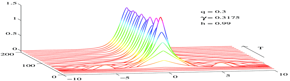
FIG. 1.: A stable pinned soliton spontaneously created from a small-amplitude random spatial distribution.

This nonlinear Schrödinger (NLS) equation was previously used to model the nonlinear Faraday resonance in a long narrow water trough [11]. The inhomogeneous term $2q\delta(X)\psi$ represents a local widening (for $q>0$) or narrowing ($q<0$) of the trough. The same equation describes an easy-plane ferromagnet with a combination of a static and hf field in the easy plane [12, 8] and a biaxial ferromagnet; in both cases the inhomogeneous term accounts for an impurity spin. Equation (5) was also used in studies of the effect of phase-sensitive parametric amplifiers on solitons in optical fibers [13].

As in the spatially homogeneous case $(q=0)$ [8], for $h>\sqrt{1+\gamma^{2}}$ the zero solution $\psi=0$ is unstable against continuous spectrum excitations. “Long” impurities ($q>0$) harbour a discrete mode (here $\epsilon\ll 1$):

$\displaystyle\delta\psi=\epsilon\left(\cos\Omega T-i\frac{1+h-q^{2}}{\Omega}\sin\Omega T\right)e^{-\gamma T-q|X|},$

$\Omega^{2}=(1-q^{2})^{2}-h^{2}$. When $h>{\mathfrak{h}}_{q,\gamma}=\sqrt{(1-q^{2})^{2}+\gamma^{2}}$, this localized mode also produces instability. For positive $q<\sqrt{2}$, in which case ${\mathfrak{h}}_{q,\gamma}$ lies below $\sqrt{1+\gamma^{2}}$, the nonlinear development of this instability leads to the formation of solitons (fig.1), stable or unstable.

Equation (5) exhibits two stationary soliton solutions, each having a cusp at the origin:

$$\psi_{\pm}(X)=A_{\pm}{\rm sech}\left(A_{\pm}|X|+{\tilde{x}}\right)e^{-i\theta_{\pm}},$$ (6)

where $\cos{2\theta_{\pm}}=\pm\sqrt{1-\gamma^{2}/h^{2}}$, $A_{\pm}^{2}=1\pm\sqrt{h^{2}-\gamma^{2}}$, ${\tilde{x}}={\rm arctanh}\left({q/A_{\pm}}\right)$. For weak impurities, $|q|<1$, the $\psi_{+}$ soliton exists for any $h$ and $\gamma$ satisfying $h>\gamma$, whereas the $\psi_{-}$ requires, in addition, that $h<{\mathfrak{h}}_{q,\gamma}$. Strong impurities ($|q|>1$) do not support the $\psi_{-}$ soliton at all whereas the $\psi_{+}$ exists only if $h>{\mathfrak{h}}_{q,\gamma}$.

First we demonstrate that the soliton $\psi_{-}$ is unstable and can always be disregarded. Taking the linear perturbation in the form $\delta\psi_{\pm}=A_{\pm}(f+ig)e^{-i\theta_{\pm}-\gamma T}$ gives

$$-g_{t}-\Gamma g=L_{1}f,\quad f_{t}-\Gamma f=L_{0}g,$$ (7)

where $\Gamma=\gamma/A_{\pm}^{2}$, $t=A_{\pm}^{2}T$, and the operators

$$L_{1}=-\partial_{x}^{2}+1-6{\rm sech}^{2}(|x|+{\tilde{x}})-2Q\delta(x),$$ (8)

$$L_{0}=-\partial_{x}^{2}+1\mp 2H-2{\rm sech}^{2}(|x|+{\tilde{x}})-2Q\delta(x),$$ (9)

with $Q=q/A_{\pm}=q\sqrt{1\mp H}$, $H=\sqrt{h^{2}-\gamma^{2}}/A_{\pm}^{2}$, and $x=A_{\pm}X$. The minimum eigenvalue of the operator $L_{0}$ associated with a nodeless eigenfunction ${\rm sech\/}(|x|+{\tilde{x}})$, is $\nu_{0}=\mp 2H$. Consequently, in the case of the $\psi_{-}$ soliton $L_{0}$ is positive definite and Eqs.(7) can be rewritten as

$$L_{0}^{-1}f_{tt}=\Gamma^{2}L_{0}^{-1}f-L_{1}f.$$ (10)

The maximum exponential growth rate $\lambda$ of solutions to Eq.(10) is given by [14]

$$\lambda^{2}=\Gamma^{2}+\sup_{f}\frac{<f(x)|-L_{1}|f(x)>}{<f(x)|L_{0}^{-1}|f(x)>}.$$ (11)

For any $Q$ the operator $L_{1}$ has a negative eigenvalue $\mu_{0}=1-\kappa^{2}$ associated with an even eigenfunction

$$y_{0}(x)=e^{-\kappa\xi}(3\tanh^{2}\xi+3\kappa\tanh\xi+\kappa^{2}-1),$$ (12)

where $\xi=|x|+{\tilde{x}}$ and $\kappa>1$ is a root of $\kappa^{3}+2\kappa^{2}Q+\kappa(3Q^{2}-5Q-4)+3Q^{3}=0$. Thus the supremum in (11) is positive, $\lambda$ is $>\Gamma$ and the soliton $\psi_{-}$ is unstable against a symmetric nonoscillatory mode for all $q$, $h$ and $\gamma$.

A similar argument can be used to detect the disengagement instability of the other soliton, $\psi_{+}$, arising for “short” impurities ($q<0$). We simply notice that the second lowest eigenvalue of $L_{0}$ which is associated with an odd eigenfunction

$\displaystyle w_{1}(x)=\mbox{sgn}(x)e^{Q(|x|+{\tilde{x}})}\left\{\mbox{tanh}(|x|+{\tilde{x}})-Q\right\},$

is equal to $\nu_{1}=1-2H-Q^{2}$. For $2H<1-Q^{2}$ or equivalently for $h<{\mathfrak{h}}_{q,\gamma}$, the operator $L_{0}$ is positive definite on the subspace of odd functions. On the other hand, for $Q<0$ the operator $L_{1}$ has a negative eigenvalue $\mu_{1}=1-\kappa^{2}$ associated with an odd eigenfunction $y_{1}(x)={\rm sgn\/}x\ y_{0}(x)$, with $y_{0}$ as in (12) and $\kappa>1$ a root of $\kappa^{2}+3\kappa Q+3Q^{2}-1=0$. Hence the variational principle (11) is still applicable, $\lambda$ is $>\Gamma$ and the $\psi_{+}$ is unstable. The interpretation of this instability is straightforward if one notices that in the conservative case ($\gamma=0$) the inhomogeneous term $-2q\delta(X)|\psi|^{2}$ produces a local decrease respectively increase of energy for $q>0$ respectively $q<0$. Consequently, in the conservative and weakly dissipative cases, the “long” impurity will attract and the “short” one repel small-amplitude tails of distant solitons. On the other hand, the energy of the pinned soliton is $E_{Q}=\frac{4}{3}A^{3}(1-3Q+2Q^{3})$. For $Q>0$ ($Q<0$) this is smaller (greater) than the energy $E_{0}$ of the infinitely remote soliton. These two facts indicate that $Q>0$-impurities should attract and trap solitons (cf.[15]). In the $Q<0$ case, conversely, distant solitons will be repelled while an initially pinned soliton will depin and move away from the impurity regaining its cusp-free shape.

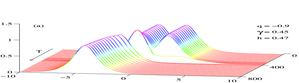
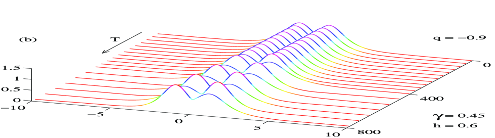
FIG. 2.: The effect of the $q<0$ impurity. For $h<{\mathfrak{h}}_{q,\gamma}$, the growth of the asymmetric instability leads to the soliton’s depinning and repulsion from the impurity (a), while for $h>{\mathfrak{h}}_{q,\gamma}$, the asymmetric Hopf instability evolves into a two-humped soliton staggering in a seesaw fashion (b).

This was indeed confirmed by simulations of Eq.(5) (fig.2(a)). It is fitting to note that the depinning instability is not connected with overdriving the chain; it occurs already in the undriven NLS [15].

In the region $h>{\mathfrak{h}}_{q,\gamma}$ (as well as in the case of symmetric instabilities, and for long impurities $q>0$) the variational principle (11) is not applicable. Here we let $f(x,t)=u(x)e^{i\Omega t}$ and $g(x,t)=-\frac{\omega}{\Gamma+i\Omega}v(x)e^{i\Omega t}$, where $\Omega^{2}=\omega^{2}-\Gamma^{2}$. Eq.(7) reduces to an eigenvalue problem

$$L_{1}u=\omega v,\quad L_{0}v=\omega u,$$ (13)

which we solved numerically. Notice that we have reduced a three- to two-parametric problem. Having found $\omega=\omega(q,H)$, one immediately recovers the instability growth rate $|{\rm Im}\,\Omega(q,H)|-\Gamma$ for all $q$, $h$, and $\gamma$.

For small $h<{\mathfrak{h}}_{q,\gamma}$ there is only one unstable pair of imaginary eigenvalues $\pm\omega_{1}$, with the associated $u$ and $v$ being odd. As $h$ is increased beyond ${\mathfrak{h}}_{q,\gamma}$, the imaginary eigenvalues move onto the real axis (i.e. the soliton restabilizes) while another real doublet $\pm\omega_{2}$ detaches from the continuous spectrum. The two collide and emerge as a complex quadruplet after which the real and imaginary parts grow until an asymmetic instability sets in. This is now not a disengagement instability; the stationary soliton is replaced by a two-humped structure (still pinned

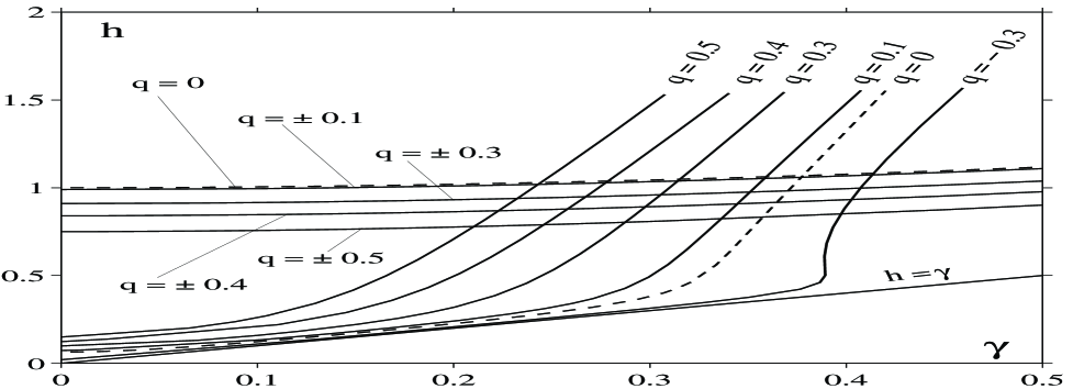
FIG. 3.: Atlas of stability charts on the $(\gamma,h)$-plane. Above the dashed “horizontal” curve, $h=\sqrt{1+\gamma^{2}}$, all localized solutions are unstable w.r.t. continuous spectrum waves. Solid “horizontal” curves are $h={\mathfrak{h}}_{q,\gamma}$. Below their corresponding ${\mathfrak{h}}_{q,\gamma}$-curves impurities with $q<0$ repel solitons. The family of “parabolas” depict the onset of (symmetric) instability of the pinned soliton; the greater is $q$ the larger is the stability domain. Finally, in the region between $\sqrt{1+\gamma^{2}}$ and ${\mathfrak{h}}_{q,\gamma}$ a $q>0$-impurity will spontaneously nucleate solitons.

on the impurity) whose left and right wings oscillate $180^{\circ}$ out of phase (fig.2(b)).

When $q>0$, the motion of eigenvalues $\omega$ on the complex plane is similar to the homogeneous case [8]. The soliton $\psi_{+}$ is stable for $h$ close to $\gamma$ but loses its stability to a symmetric oscillating soliton as $h$ is increased. Fig.3 shows the Hopf bifurcation curves $h=h_{q}(\gamma)$ obtained from the relation $|{\rm Im}\,\Omega(q,H)|=\Gamma$ for $q=0.1,\,0.3,\,0.4,\,0.5$ and $-0.3$. For $q>0$ the stability domain is wider than without an impurity. For example, in a chain with the coupling $k=0.5$ driven at $\omega\approx 0.98$, lengthening the central pendulum by 15% (which gives $q=0.5$) is sufficient to double the size of the soliton’s stability domain. If the same chain is driven at $\omega\approx 0.999$, the $q=0.5$ and hence the same effect is produced just by a 3% elongation of the central pendulum. On the contrary, the $q<0$ impurity narrows the stability domain.

Thus, long impurities exert a strong influence on solitons’ dynamics. For $h<{\mathfrak{h}}_{q,\gamma}$ they attract and trap solitons; for $h>{\mathfrak{h}}_{q,\gamma}$ pinned solitons are spontaneously formed around the $q>0$ defects. On the other hand, the soliton with $h$ and $\gamma$ such that it would ignite spatiotemporal chaos in the homogeneous case [9], is stabilized when pinned on a sufficiently long impurity (fig.4). Therefore the $q>0$ defects should have a stabilizing effect on the chain. One should keep in mind, however, that spatiotemporal chaotic states are not localized and

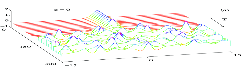
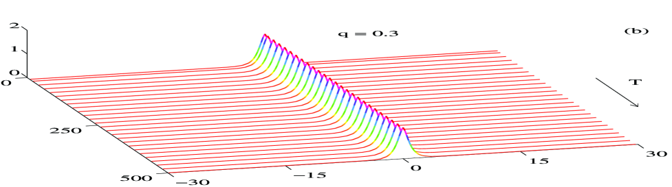
FIG. 4.: In the homogeneous chain with $\gamma=0.315,h=0.95$ the unstable soliton seeds spatiotemporal chaos (a). Introducing the impurity with $q=0.3$ is sufficient to stabilize it (b).

a single stable soliton will clearly be insufficient to suppress chaos in a long chain. The chaos can always be triggered by choosing the initial condition far enough from the soliton. In order to suppress chaos in a larger phase volume multiple impurities should be introduced; one is therefore led to the necessity of examining stability of solitons and periodic waves on finite intervals.

Next, the fact that short impurities enhance the symmetric instability should not play a destabilizing role since solitons tend to avoid “short” defects. On the contrary, these repulsive inhomogeneities will effectively partition the chain into smaller intervals and this will generally have a stabilizing effect since long-wavelength instabilities will not fit in [16].

The analysis of the effect of multiple impurities (as well as the related case of finite intervals) is beyond the scope of this work. Here we only mention that introducing more than one impurity can result in more complicated (though still regular) patterns. We illustrate this by simulating the case of two impurities. As one could expect, when two stable stationary solitons are pinned very far from each other, they do not interact and remain time-independent. However, if the separation is smaller than a certain critical distance, they start exchanging weak radiation waves and develope spontaneous oscillations which subsequently synchronize (fig.5.)

This research was supported by the FRD of South Africa, Max-Planck-Gesellschaft and FORTH of Greece.

FIG. 5.: Two $q>0$ impurities placed in the middle and at the end of the periodic interval, respectively.

REFERENCES

- [1] On leave from Department of Mathematics, University of Cape Town, Private Bag Rondebosch 7701, South Africa.
- [2] Email: nora,igor@mpipks-dresden.mpg.de
- [3] Email: gts@physics.uch.gr
- [4] Y. Braiman, W.L. Ditto, K. Wiesenfeld, and M.L. Spano, Phys. Lett. A 206, 54 (1995)
- [5] Y. Braiman, J.F. Lindner and W.L. Ditto, Nature (London) 378, 465 (1995)
- [6] G.V. Osipov and M.M. Sushchik, IEEE Trans. Circuits Syst., I: Fundam. Theory Appl. 44, 1006 (1997)
- [7] A. Gavrielides, T. Kottos, V. Kovanis and G. P. Tsironis, Phys. Rev. E 58, 5529 (1998)
- [8] I.V. Barashenkov, M.M. Bogdan, and V.I. Korobov, Europhys. Lett. 15, 113 (1991).
- [9] M. Bondila, I.V. Barashenkov, and M.M. Bogdan, Physica D 87, 314 (1995)
- [10] N.V. Alexeeva, I.V. Barashenkov and D.E. Pelinovsky, Nonlinearity 12, 103 (1999).
- [11] J.W. Miles, J. Fluid Mech. 148, 451 (1984); M. Umeki, J. Phys. Soc. Jpn. 60, 146 (1991); J. Fluid Mech. 227, 161 (1991); X. Wang and R. Wei, Phys. Rev. Lett. 78, 2744 (1997)
- [12] V.E. Zakharov, V.S. L’vov and S.S. Starobinets, Sov. Phys. Uspekhi 17, 896 (1975); M.M. Bogdan, A.M. Kosevich and I.V. Manzhos, Sov. J. Low Temp. Phys. 11, 547 (1985); H. Yamazaki and M. Mino, Prog. Theor. Phys. Suppl. 98, 400 (1989)
- [13] I.H. Deutsch and I. Abram, J. Opt. Soc. Am. B11, 2303 (1994); A. Mecozzi, L. Kath, P. Kumar, and C.G. Goedde, Opt.Lett. 19, 2050 (1994); S. Longhi, Opt.Lett. 20, 695 (1995); Phys. Rev. E 55, 1060 (1997).
- [14] G. Laval, C. Mercier and R. Pellat, Nucl. Fusion 5, 156 (1965); E.M. Barston, Phys. Fluids 12, 2162 (1969); J. Fluid Mech. 42, 97 (1970)
- [15] M.M. Bogdan, A.S. Kovalev, and I.V. Gerasimchuk, Low Temp. Phys. 23, 145 (1997)
- [16] An example of the soliton stabilization through the interval shortening is discussed in I.V. Barashenkov and Yu.S. Smirnov, Phys. Rev. E 54, 5707 (1996)