Stability of Multi-hump Optical Solitons

Abstract

We demonstrate that, in contrast with what was previously believed, multi-hump solitary waves can be stable. By means of linear stability analysis and numerical simulations, we investigate the stability of two- and three-hump solitary waves governed by incoherent beam interaction in a saturable medium, providing a theoretical background for the experimental results reported by M. Mitchell, M. Segev, and D. Christodoulides [Phys. Rev. Lett. 80, 4657 (1998)].

Self-guided optical beams, or spatial optical solitons, are the building blocks of all-optical switching devices where light itself guides and steers light without fabricated waveguides [1]. In the simplest case, a spatial soliton is created by one beam of a certain polarization and frequency, and it can be viewed as a self-trapped mode of an effective waveguide it induces in a medium [2]. When a spatial soliton is composed of two (or more) modes of the induced waveguide [3], its structure becomes rather complicated, and the soliton intensity profile may display several peaks. Such solitary waves are usually referred to as multi-hump solitons; they have been found for various nonlinear models of coupled fields [4].

In realistic (nonintegrable) physical models, solitary waves can become unstable demonstrating self-focusing, decay, or a nonlinearity-driven transition to a stable state, if the latter exists [5]. All these scenarios of soliton evolution are initiated by exponentially growing perturbations and they are attributed to linear instability. It is usually believed that all types of multi-hump solitary waves are linearly unstable, except for the special case of neutrally stable solitons in the integrable Manakov model [6]. On the contrary, recent experimental results [7] indicate the possibility of observing stationary structures resembling multi-hump solitary waves. This naturally poses a question: Were those observations only possible because of short propagation distance and a small instability growth rate? Definitely, the experimental results challenge the conventional view on multi-hump solitary waves in different models of nonlinear physics.

The purpose of this Letter is twofold. First, we study the origin of multi-hump solitons supported by incoherent interaction of two optical beams in a photorefractive medium. We find that multi-hump solitons appear via bifurcations of one-component solitons and due to the process of hump multiplication, when the intensity profile of a composite soliton changes from single- to multi-humped with increasing power. Second, we perform numerical stability analysis of two- and three-hump solitary waves and also find analytically the instability threshold for two-hump solitons. We reveal that two-hump solitary waves are linearly stable in a wide region of their existence, whereas all three-hump solitons are linearly unstable, and that even linearly stable multi-hump solitons may not survive collisions.

In the experiments [7], spatial multi-hump solitary waves were generated by incoherent interaction of two optical beams in a biased photorefractive crystal. The corresponding model has been derived by Christodoulides et al. [8], and it is described by a system of two coupled nonlinear equations for the normalized beam envelopes, $u(x,z)$ and $w(x,z)$, which for the purpose of our current analysis can be written in the following form [9]:

$$\begin{array}[]{l}{\displaystyle i\frac{\partial u}{\partial z}+\frac{1}{2}\frac{\partial^{2}u}{\partial x^{2}}+\frac{u(|u|^{2}+|w|^{2})}{1+s(|u|^{2}+|w|^{2})}-u=0,}\\[9.0pt] {\displaystyle i\frac{\partial w}{\partial z}+\frac{1}{2}\frac{\partial^{2}w}{\partial x^{2}}+\frac{w(|u|^{2}+|w|^{2})}{1+s(|u|^{2}+|w|^{2})}-\lambda w=0,}\end{array}$$ (1)

where the transverse, $x$, and propagation, $z$, coordinates are measured in the units of $(L_{d}/k)^{1/2}$ and $L_{d}$, respectively, $L_{d}$ is a diffraction length, and $k$ is the wavevector in the medium. The parameter $\lambda$ is a ratio of the nonlinear propagation constants, and $s$ is an effective saturation parameter. For $s\rightarrow 0$, the system (1) reduces to the integrable Manakov equations [6].

We look for stationary, $z$-independent, solutions of Eqs. (1) with both components $u(x)$ and $w(x)$ real and vanishing as $|x|\rightarrow\infty$. Different types of such two-component localized solutions, existing for $0<\{\lambda,s\}<1$, can be characterized by the total power, $P(\lambda,s)=P_{u}+P_{w}$, where the partial powers, $P_{u}=\int_{-\infty}^{\infty}|u|^{2}dx$ and $P_{w}=\int_{-\infty}^{\infty}|w|^{2}dx$, are integrals of motion. If one of the components is small, i.e. $w/u\sim\varepsilon$, Eqs. (1) become decoupled and, in the leading order, the equation for the $u$-component has a solution $u_{0}(x)$ in the form of a fundamental, $sech$-like, soliton with no nodes. The second equation can then be considered as an eigenvalue problem for the “modes” $w_{n}(x)$ of a waveguide created by the soliton $u_{0}(x)$ with the effective refractive index profile $u^{2}_{0}(x)/[1+su^{2}_{0}(x)]$. Parameter $s$ determines the total number of guided modes and the cut-off value for each mode, $\lambda_{n}(s)$. Therefore, a two-component vector soliton $(u_{0},w_{n})$ consists of a fundamental soliton and an $n$th-order mode of the waveguide it induces in the medium. Henceforward we denote such a composite solitary wave by its “state vector”: $|0,n\rangle$.

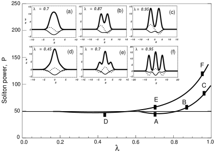
FIG. 1.: Soliton bifurcation diagram for $s=0.8$. Horizontal line - branch of the fundamental $u-$soliton. A-B-C - branch of $|0,1\rangle$ solitons. D-E-F - branch of $|0,2\rangle$ solitons. Inset: Transverse profiles of $u$- (thin), $w$- (dashed) fields, and total intensity (thick), shown for marked points.

On the $P(\lambda)$ diagram (for fixed $s$), continuous branches representing $|0,n\rangle$ solitons emerge at the points of bifurcations $\lambda_{n}(s)$ of one-component solitons (see Fig. 1). It is noteworthy that the first-order mode is in fact the lowest possible mode of the waveguide induced by the fundamental soliton $u_{0}(x)$. This is because the state $|0,0\rangle$, node-less in both components, can exist only in the degenerate case $\lambda=1$, when Eqs. (1) have a family of equal-width solutions $u_{0}=A(x)\sin\theta$ and $w_{0}=A(x)\cos\theta$, with arbitrary $\theta$, and amplitude $A$ satisfying the scalar equation, $dA/dx=\pm s^{-1}[\log(1+sA^{2})-s(1-s)A^{2}]^{1/2}$.

Additionally, indefinitely many families of vector solitons $|m,n\rangle$, where $m\neq n\neq 0$, can be formed as bound states of phase-locked $|0,n\rangle$ solitons [10, 11]. Although such states do contribute to the rich variety of the multi-hump solitons existing in our model, we exclude them from our present consideration.

Families of vector solitons can be found by numerical relaxation technique. Some results of our calculations are presented in Fig. 1, for $|0,1\rangle$ and $|0,2\rangle$ solitons found at $s=0.8$. Observing the modification of soliton profiles with changing $\lambda$ (see inset in Fig. 1), one can see that the modal description of two-component solitons is valid only near bifurcation points. For $\lambda\gg\lambda_{n}$, the amplitude of an initially small $w$-component grows and the soliton-induced waveguide deforms. It is this purely nonlinear effect that gives rise to the existence of multi-hump solitons. In particular, two- and three-hump solitons are members of the soliton families $|0,1\rangle$ (branch A-B-C) and $|0,2\rangle$ (branch D-E-F) originating at different bifurcation points. At $\lambda\sim\lambda_{n}(s)$, while the $w$-component remains small, all $|0,n\rangle$ solitons are single-humped, as shown in Figs. 1(a,d). As the amplitude of $w$ grows with increasing $\lambda$, the total intensity profile, $I(x)=u^{2}_{0}(x)+w^{2}_{n}(x)$, develops $(n+1)$ humps [see Figs. 1(b,e)], and at sufficiently large $\lambda$ the $u$-component itself becomes multi-humped [Figs. 1(c,f)]. The separation distance between the soliton humps tends to infinity as $\lambda\rightarrow 1$.

To analyze the linear stability of multi-hump solitons, we seek solutions of Eqs. (1) in the form of weakly perturbed solitary waves: $u(x,z)=u_{0}(x)+\varepsilon[F_{u}(x,z)+iG_{u}(x,z)]$ and $w(x,z)=w_{n}(x)+\varepsilon[F_{w}(x,z)+iG_{w}(x,z)]$, where $\varepsilon\ll 1$. Setting $F_{u,w}\sim f_{u,w}(x)e^{\beta z}$, $G_{u,w}\sim g_{u,w}(x)e^{\beta z}$, one can obtain the following eigenvalue problem (EVP)

$$\hat{\mathcal{L}}_{1}\hat{\mathcal{L}}_{0}\vec{g}=-\Lambda\vec{g},$$ (2)

$$\hat{\mathcal{L}}_{0}\hat{\mathcal{L}}_{1}\vec{f}=-\Lambda\vec{f}.$$ (3)

Here $\vec{g}\equiv(g_{u},g_{w})^{T}$, $\vec{f}\equiv(f_{u},f_{w})^{T}$, $\Lambda=\beta^{2}$, and

$\displaystyle\hat{\mathcal{L}}_{0,1}=\left(\begin{array}[]{cc}-\frac{1}{2}\frac{d^{2}}{dx^{2}}+1-a_{0,1}&b_{0,1}\\ b_{0,1}&-\frac{1}{2}\frac{d^{2}}{dx^{2}}+\lambda-c_{0,1}\end{array}\right),$

where $a_{0}=c_{0}=I/(1+sI)$, $b_{0}=0$, $a_{1}=a_{0}+2u_{0}^{2}/(1+sI)^{2}$, $c_{1}=c_{0}+2w_{n}^{2}/(1+sI)^{2}$, and $b_{1}=-2u_{0}w_{n}/(1+sI)^{2}$.

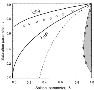
FIG. 2.: Existence and stability domains for two- and three-hump solitons. Shown are the existence thresholds $\lambda_{1}(s)$ and $\lambda_{2}(s)$ for the $|0,1\rangle$ and $|0,2\rangle$ soliton families. Dashed - the line where $|0,1\rangle$ solitons become two-humped. Shaded - analytically obtained instability domain for two-hump solitons. Squares and circles- numerically obtained instability thresholds for $|0,1\rangle$ and $|0,2\rangle$ solitons, respectively.

Because $\hat{\mathcal{L}}_{1}\hat{\mathcal{L}}_{0}$ and $\hat{\mathcal{L}}_{0}\hat{\mathcal{L}}_{1}$ are adjoint operators with identical spectra, we can consider the spectrum of only one of these operators, e.g. $\hat{\mathcal{L}}_{1}\hat{\mathcal{L}}_{0}$. Considering the complex $\Lambda$-plane, it is straightforward to show that $\Lambda\in(-\infty,-\lambda^{2})$ is a continuum part of the spectrum with unbounded eigenfunctions. Stable bounded eigenmodes of the discrete spectrum (the so-called soliton internal modes [12]) can have eigenvalues only inside the gap, $-\lambda^{2}<\Lambda<0$. The presence of either positive or complex $\Lambda$ implies soliton instability, because in this case there always exists at least one eigenvalue of the soliton spectrum with ${\rm Re}\beta>0$.

Numerical solution of the EVP (2) shows that both $|0,1\rangle$ and $|0,2\rangle$ types of solitary wave solutions can be stable in a certain region of their existence domain, see Fig. 2. In the case of $|0,1\rangle$ solitons, the appearance of the instability is related to the fact that close to the curve where the total intensity $I$ becomes two-humped [dashed line in Fig. 2], a pair of internal modes split from the continuum into the gap. As $\lambda$ grows, the corresponding, purely imaginary, eigenvalues $\beta=\pm i{\sqrt{|\Lambda(\lambda)|}}$ tend to zero, and at a certain critical value $\lambda=\lambda_{\rm cr}(s)$, they coincide at $\beta=0$. At this point, an eigenmode with positive eigenvalue $\Lambda$ emerges, thus generating linear instability (see Fig. 3) with the instability growth rate $\beta=\sqrt{\Lambda(\lambda)}$. For $|0,2\rangle$ solutions, the dynamics of internal modes can not be related in any obvious way with a change in the spatial solitary profiles, nevertheless the scenario of the instability development is similar to that for two-hump solitons. The dependence of $\beta$ on $\lambda$, for $|0,1\rangle$ and $|0,2\rangle$ soliton families giving rise to two- and three-hump solitary waves, is shown in Fig. 3 for $s=0.3$ and $s=0.8$, respectively. A decline in the instability growth rate as $\lambda\rightarrow 1$ (see Fig. 3) is caused by the fact that, in this limit, all multi-hump solitons decompose into a number of the neutrally stable $|0,0\rangle$ solitons separated by infinitely growing distance. Numerical analysis in the close vicinity of this limit is unfeasible due to lack of computational accuracy.

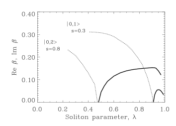
FIG. 3.: Instability eigenvalues vs. $\lambda$ for $|0,1\rangle$ and $|0,2\rangle$ solitons; dashed line - ${\rm Im}\beta$, bold line - ${\rm Re}\beta$.

Note that, within the gap of the continuous spectrum, there exist several soliton internal modes not participating in the development of the linear instability. Analysis of their origin and influence on the soliton dynamics is beyond the scope of the present Letter.

With the aid of analytical asymptotic technique [13], it is possible to show that a perturbation mode with small but positive eigenvalue, and therefore the linear instability of a general localized solution $(u,w)$, appears if the functional $J(u,w),$ defined as

$$J=\frac{P_{u}}{2s}\frac{\partial P_{w}}{\partial\lambda}-\frac{P_{w}}{2s}\frac{\partial P_{u}}{\partial\lambda}+\frac{\partial P_{u}}{\partial s}\frac{\partial P_{w}}{\partial\lambda}-\frac{\partial P_{w}}{\partial s}\frac{\partial P_{u}}{\partial\lambda},$$ (4)

changes its sign. The threshold condition $J=0$ is, in fact, the Vakhitov-Kolokolov stability criterion [14], generalized for the case of two-parameter vector solitons. In this case, it does not necessarily give a threshold of leading instability [15]. Therefore, the presence of other instabilities (which are not associated with the condition $J=0$ and can have stronger growth rates) is still possible, as in some other cases [16].

For two-hump solitons, we have been able to locate the critical curve in $(\lambda,s)$-plane corresponding to the condition $J=0$. Superimposing this curve onto the numerically calculated values $\lambda_{\rm cr}(s)$, we have found a remarkable agreement between the numerical and analytical instability thresholds, as shown in Fig. 2. This gives us the first example of the generalized Vakhitov-Kolokolov criterion for the instability threshold of vector multi-hump solitary waves. For the whole family of $|0,2\rangle$ solutions, including three-hump solitons, it appears that $J\neq 0$ throughout the entire existence region. Thus, appearance of instability of three-hump solutions is not associated with the change of the sign of the functional $J$.

To analyze long-term evolution of multi-hump solitary waves, we perform numerical simulations of the beam propagation for $|0,n\rangle$ solitons within the existence domain $\lambda_{n}<\lambda<1$, at fixed $s$. First, we use no perturbation so that the soliton instability can only develop from numerical noise. As long as the soliton maintains its single-humped shape [see corresponding profiles in Fig. 1(a,d)], it remains almost insensitive to numerical noise. Moreover, while the $|0,1\rangle$ solitons do become two-humped at $\lambda<\lambda_{\rm cr}$, they still remain stable in a wide domain of their parameters until the linear instability threshold is reached. On the contrary, $|0,2\rangle$ solitons remain single-humped up to the instability threshold value $\lambda=\lambda_{\rm cr}$, so that all three-hump solitons are indeed unstable. Above the instability threshold (i.e. for $\lambda_{\rm cr}<\lambda<1$), a two-hump soliton splits into two independent single-humped beams as a result of the instability developed from noise [see Fig. 4(a)], whereas a three-hump soliton exhibits a more complex symmetry-breaking instability, as shown in Fig. 4(b).

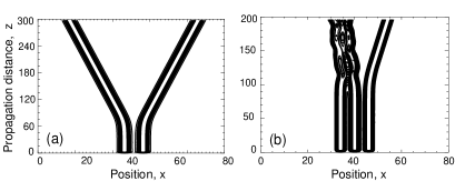
FIG. 4.: Noise-induced splitting of (a) two-hump soliton [Fig.1(c)] and (b) three-hump soliton [Fig. 1(f)].

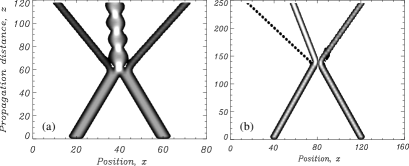
FIG. 5.: Collisions of (a) linearly stable $|0,1\rangle$ solitons at $s=0.8$, $\lambda=0.72$ with the relative transverse velocity $v=0.05$, and (b) linearly stable $|0,2\rangle$ solitons at $s=0.8$, $\lambda=0.35$, with $v=0.09$.

Next, we propagate two-hump (at $s=0.3$) and three-hump (at $s=0.8$) solitons perturbed by an eigenmode with the largest instability growth rates, i.e. $\beta_{\rm max}\approx 0.055$ and $\beta_{\rm max}\approx 0.153$, respectively. We find that in the presence of $\sim 6\%$ amplitude perturbation, the diffraction-induced decay of a soliton can be stabilized by the nonlinearity, whereas its splitting is significantly speeded up by the perturbation, compared with splitting due to a numerical noise.

To make a link between our stability analysis and experiment, we note that for the experiment [7] the diffraction length is defined as $L_{d}=2/sb$ and nonlinearity of the medium (SBN:60 crystal) is characterised by the parameter $b=kr_{\rm eff}n_{b}^{2}E_{0}$, where $r_{\rm eff}$ is the effective electro-optic coefficient ($=280$ pm/V), $n_{b}$ is the background refractive index $(=2.3)$, and $E_{0}$ is the applied electric field ($\approx 2$x$10^{5}$ V/m). For strong saturation we have $s\sim 1$ and $L_{d}\approx 0.2$mm. Now, the characteristic instability length $z_{\rm cr}$ can be defined through the maximum growth rate $\beta_{\rm max}$ and, as a result, for two-hump solitons at $s=0.3$ we obtain $z_{\rm cr}\approx 12.18$ mm. These estimates indicate that the instability, if it exists, could be detected for two-hump solitons within the experimental setup of Ref. [7] and therefore stable two-hump solitons have been indeed observed.

Importantly, three-hump solitons so far generated in the experiment belong to a different class of vector solitons which, in our notation, can be identified as $|1,2\rangle$ states. The extensive numerical analysis of soliton states $|1,2\rangle$ [11] shows that all such solitons are linearly unstable. However, the observation of this instability is beyond the experimental parameters of Ref. [7].

The complex structure of multi-hump solitons and nonintegrability of the model (1) result in a variety of collision scenarios, which are quite dissimilar to the collisions of multi-hump solitons of the exactly integrable Manakov system [6]. For instance, even linearly stable vector solitons do not necessarily survive soliton collisions. In Figs. 5(a,b) we show two examples of non-elastic interaction of linearly stable $|0,1\rangle$ and $|0,2\rangle$ solitons.

In conclusion, we have analyzed, analytically and numerically, the stability of multi-hump optical solitons in a saturable nonlinear medium. We have found that multi-hump solitons are members of an extended class of vector solitons which can be linearly stable in a wide region of their existence, although they may be destroyed in collisions. We believe that this is an important physical result that calls for a revision of our understanding of the structure and stability of many types of multi-hump solitary waves in nonintegrable multi-component models, usually omitted in the analysis because of their a priori assumed instability.

We thank M. Segev, D. Christodoulides, M. Mitchell, and A. Buryak for useful discussions. Yu.K. and E.O. are members of the Australian Photonics Cooperative Research Centre. D.S. acknowledges support from the Royal Society of Edinburgh and British Petroleum.

REFERENCES

- [1] M. Segev and G.I. Stegeman, Phys. Today 51, 42 (1998).
- [2] R.Y. Chiao, E. Garmire, and C.H. Townes, Phys. Rev. Lett. 13, 479 (1964).
- [3] A.W. Snyder, S.J. Hewlett, and D.J. Mitchell, Phys. Rev. Lett. 72, 1012 (1994).
- [4] See, e.g, I. A. Kol’chugina et al., JETP Lett. 31, 6 (1980); M. Haelterman and A.P. Sheppard, Phys. Rev. E 49, 3376 (1994); J.M. Soto-Crespo et al., Phys. Rev. E 51, 3547 (1995); A. Boardman et al., Phys. Rev. A 52, 4099 (1995); D. Michalache et al., Opt. Eng. 35, 1616 (1996); H. He et al., Phys. Rev. E 54, 896 (1996).
- [5] See, e.g., D.E. Pelinovsky, V.V. Afanasjev, and Yu. S. Kivshar, Phys. Rev. E 53, 1940 (1996).
- [6] S.V. Manakov, Sov. Phys. JETP 38, 248 (1974); see also V. Kutuzov et. al., Phys. Rev. E 57, 6056 (1998); N. Akhmediev, W. Krolikowski, and A.W. Snyder, Phys. Rev. Lett. 81, 4632 (1998).
- [7] M. Mitchell, M. Segev, and D.N. Christodoulides, Phys. Rev. Lett. 80, 4657 (1998).
- [8] D.N. Christodoulides et al., Appl. Phys. Lett. 68, 1763 (1996).
- [9] E.A. Ostrovskaya and Yu.S. Kivshar, Opt. Lett. 23, 1268 (1998).
- [10] E.A. Ostrovskaya and Yu.S. Kivshar, J. Opt. B: Quantum Semiclass. Opt. 1, 77, (1999).
- [11] E.A. Ostrovskaya, PhD Thesis, The Australian National University, (1999).
- [12] Yu.S. Kivshar et al., Phys. Rev. Lett. 80, 5032 (1998).
- [13] A.V. Buryak, Yu.S. Kivshar, and S. Trillo, Phys. Rev. Lett. 77, 5210 (1996).
- [14] M.G. Vakhitov and A.A. Kolokolov, Sov. Radiophys. 16, 783 (1973).
- [15] V.G. Makhankov, Y.P. Rybakov, and V.I. Sanyuk, Physics-Uspekhi 37, 113 (1994).
- [16] D.V. Skryabin and W.J. Firth, Phys. Rev. E 58, R1252 (1998); P. Lundquist, D. R. Andersen, and Yu. S. Kivshar, Phys. Rev. E 57, 3551 (1998); D. Mihalache, D. Mazilu, and L. Torner, Phys. Rev. Lett. 81, 4353 (1998).