[

On-off Intermittency in Stochastically Driven Electrohydrodynamic Convection in Nematics

Abstract

We report on-off intermittency in electroconvection of nematic liquid crystals driven by a dichotomous stochastic electric voltage. With increasing voltage amplitude we observe laminar phases of undistorted director state interrupted by shorter bursts of spatially regular stripes. Near a critical value of the amplitude the distribution of the duration of laminar phases is governed over several decades by a power law with exponent $-3/2$. The experimental findings agree with simulations of the linearized electrohydrodynamic equations near the sample stability threshold.

]

Systems at a threshold of stability driven by a stochastic or chaotic process coupling multiplicatively to the system variables may exhibit on-off intermittency characterized by specific statistical properties of the intermittent signal. Quiescent (or laminar) periods (off-states) are interrupted by bursts of large variation (on-states); the duration of laminar periods is governed by power laws with exponents universal over a broad class of different systems. Early theoretical studies considered systems with few degrees of freedom modeled by differential equations [1] and mappings [2]. There is increasing interest in systems with many degrees of freedom [3], described by random map lattices [4], larger systems of coupled nonlinear elements [5], and partial differential equations [5, 6]. Experimental results are available mainly for nonlinear electric circuits [7]; on-off intermittency was also observed in a spin wave experiment [8], in optical feedback [9], and a gas discharge plasma system [10]. Here we first report about on-off intermittency in a spatially extended dissipative system, viz. electroconvection (EC) in nematic liquid crystals driven by a stochastic voltage.

EC in planarly aligned nematics is a standard system for pattern formation, for recent reviews see, e.g. [11]. In the presence of an electric field $E$ a spontaneous fluctuation of the director leads due to the anisotropic conductivity to a formation of space charges which tend to destabilize the homogeneously ordered state. With increasing strength of the driving field one observes a hierarchy of convection patterns of increasing complexity. The patterns depend on external parameters such as amplitude, frequency and wave form of the driving voltage which are conveniently adjustable in the experiment. The hydrodynamic flow induces a modulation of the director field and thus of the effective indices of refraction which leads to transmission patterns easily observed with a microscope.

In previous experiments, the superposition of a deterministic AC field with a stochastic field, $E=E^{det}(t)+E^{stoch}(t)$, was studied. A variety of noise induced phenomena including stabilization or destabilization of the homogeneous state, and a change from continuous to discontinuous behaviour of the threshold as a function of the noise strength was observed [12, 13, 14, 15, 16] and has stimulated theoretical work [17, 18].

As long as the characteristic time of the noise $\tau_{\text{stoch}}$ is small compared with characteristic times of the system the threshold towards pattern formation appears sharp as for deterministic driving. It is however typical for EC in nematics that one of the systems characteristic times decreases both with increasing strength of the threshold voltage and with increasing wave number of the pattern and may reach the order of $\tau_{\text{stoch}}$ [18]. In this case, one observes intermittent bursts of a regular spatial stripe pattern which makes a naïve experimental determination of the stochastic threshold difficult [16]. A similar phenomenon was noticed in a highly doped nematic material for very high strength of the noise [13] where a direct transition towards chaos occurs via intermittent bursts of spatially incoherent structures embedded in a homogeneous background.

In this paper, we consider the simplest case of pure stochastic excitation, $E=E^{stoch}(t)$. To achieve a statistical characterization we have determined experimentally the distribution of the duration $\tau$ of laminar, i.e. undistorted phases (off-states) which are interrupted by bursts of a stripe pattern (on-states). Approaching a critical voltage from below, this distribution is governed by a power law $\tau^{-3/2}$ over several orders of $\tau$ as it is typical for on-off-intermittency. This result is confirmed by simulations of the linearized electrohydrodynamic equations at the sample stability threshold [18].

We use the standard experimental set-up with a commercial cell (Linkam) providing planar anchoring of the director by antiparallely rubbed polyimide coatings, two transparent ITO electrodes of 5$\times$5mm² and a cell gap of $d=50\mu$m. The nematic material is a mixture of four disubstituted phenylbenzoates [16] which has a nematic range from below room temperature to 70.5^∘C. The cell temperature is controlled at $30^{\circ}$C by a Linkam heating stage. Images are recorded using a Jenapol-d polarizing microscope and a Hamamatsu B/W camera with controller C2400. The transmission images of light polarized along the director easy axis $\vec{n}_{0}$ are recorded digitally. We resolve the images in 500$\times$400 (330$\times$250) pixels with 8 bits greyscale and calculate standard deviations in real time at a rate of 1/7 (1/20) s in the conductive (dielectric) regime.

As driving process we use the dichotomous Markov process (DMP) which is easily generated and faciliates the theoretical analysis. The DMP $E_{t}^{\text{DMP}}$ jumps randomly between $\pm E$ with average rate $\alpha$. The distribution of times $\tilde{\tau}$ between two consecutive jumps is $\alpha\exp{(-\alpha\tilde{\tau})}$; the autocorrelation decays exponentially, $<E_{t}^{\text{DMP}}E_{t^{\prime}}^{\text{DMP}}>=E^{2}\exp[-2\alpha(t-t^{\prime})]{}$, i.e. $\tau_{\text{stoch}}=1/2\alpha$. We will refer to $\nu=\alpha/2$ as the mean frequency and to $E$ as the amplitude of the noise. Both in experiment and simulation, sequences of the DMP are generated by the same algorithm; technically $\tilde{\tau}$ is limited to vary between $10^{-4}$s and $10^{4}$s.

For excitation by a periodic square wave, one finds a typical frequency dependent threshold voltage $U_{c}$ ($U=Ed$) for the stability against formation of normal rolls, cf. Fig. 1. There is a sharp transition at $\nu_{c}=38$ Hz between the conductive regime (oscillating space charges) characterized by a wavenumber $k_{x}\approx\pi/d$ and the dielectric regime (oscillating director deflections), where $k_{x}$ is an order of magnitude larger, cf. Fig. 1.

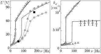
FIG. 1.: Threshold voltages and wave numbers for driving with periodic and stochastic square waves of (mean) frequency $\nu$. Experimental data (diamonds: periodic case; circles, triangles, and full squares: stochastic case, see text; dashed lines guide the eyes) are compared with results from the two-dimensional theory (full line: periodic case; dotted line: stochastic case).

For stochastic driving, we have observed bursts of stripe pattern uniform across the system already below the onset threshold for a periodic voltage of the same frequency. The stochastic voltage has a broad frequency spectrum which contains low frequency contributions. Occasional bursts of convective pattern can be expected at voltages above the DC threshold ($\nu=0$ in Fig. 1a). With increasing voltage the frequency of the bursts increases. In Fig. 1a we have plotted the voltages which correspond to a ratio of 75% (circles) and 25% (triangles) of laminar phases, respectively. The full squares at $\nu=60$ Hz and 180 Hz indicate the voltages for which the experimentally determined distribution of laminar periods $\tau$ is best described by a $\tau^{-3/2}$ law (see below). The theoretical results obtained from the sample stability criterion explained below agree very well with the experimental data. (Both in the periodic and the stochastic case we have used the same material parameters.)

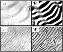
FIG. 2.: Snapshots of the bursts of roll patterns (a, b) in the conductive regime ($\nu=60$ Hz, $k_{x}=1.2\times 10^{3}$ cm^-1, area size 200$\times 164\,\mu$m²) and (c, d) in the dielectric regime ($\nu=180$ Hz, $k_{x}=7.2\times 10^{3}$cm^-1, area size 134$\times 102\,\mu$m²) at different times. (a, c) show the patterns just at the threshold of the on-state ($\sigma_{\text{rel}}=0.1$) whereas in (b, d) the rolls are fully developed ($\sigma_{\text{rel}}=0.8$).

The set of images in Fig. 2 shows the stripe pattern at different times of a burst just at the threshold of the on-state and the fully developed pattern in both the dielectric and the conductive regime. We characterize the intensity modulation of these patterns by $\sigma_{\text{rel}}=(\sigma-\sigma_{0})/(1-\sigma_{0})$ where $\sigma$ is the normalized standard deviation from the average intensities taken over all pixels of the image at a given instant, and $\sigma_{0}$ is the value of $\sigma$ for zero voltage. This procedure allows a real time characterization of the patterns. It is justified since the largest Fourier coefficient dominates the intensity modulation , and both quantities have nearly equivalent traces. Although the relation between $\sigma_{\text{rel}}$ and the director deflections is nonlinear, the approach used here is sufficient if we are interested only in the frequency and duration of the bursts and not primarily in their amplitudes.

In Fig. 3 we present trajectories of $\sigma_{\text{rel}}(t)$ observed in the experiment for different noise amplitudes but the same seed of the driving DMP. As laminar phase we define the period in which $\sigma_{\text{rel}}(t)$ is below a threshold $\sigma_{\text{lam}}=0.1$ where the choice of $\sigma_{\text{lam}}$ is not crucial. The laminar periods are interrupted by bursts of the convection structures, the frequency of which increases with the applied voltage amplitude $U$.

In Figs. 4 and 5 we compare the experimentally determined distributions $p(\tau)$ for the occurence of laminar phases of duration $\tau$ with those obtained in simulations in the conductive and the dielectric regime, respectively.

FIG. 3.: Bursts of the intensity modulation $\sigma_{\text{rel}}(t)$ in the conductive regime (a) just at the threshold and (b) 0.3 V above threshold for identical trajectories of the DMP which makes about $9\times 10^{4}$ jumps in the period shown ($\nu=60$ Hz). The dashed lines indicate $\sigma_{lam}$ above which the system is in the on-state and else in the off-state.

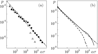
FIG. 4.: Normalized distribution $p(\tau)$ in the conductive regime ($\nu$ = 60 Hz) just at the stability threshold and slightly above. Shown are results (a) from experiment for $U=14.6$ V (squares) and $15.3$ V (triangles), and (b) from simulations for $U=U_{c}=18.2$ V (full line) and $U=19.0$ V (dashed line). Mode selection gives a wave number $k_{x}=1484$ cm^-1 used in the simulation. The dash-dotted lines indicate a power law $\tau^{-3/2}$.

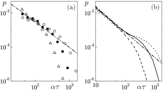
FIG. 5.: Normalized distribution $p(\tau)$ in the dielectric regime ($\nu$ = 180 Hz) slightly below $U_{c}$, just at $U_{c}$, and slightly above. Shown are (a) experimental results for $U=76.0$ V (circles), 79.5 V (squares), and 83.0 V (triangles), and (b) simulations for $U=82.0$ V (dotted line), $U=U_{c}=84.9$ V (full line), and $U=90.0$ V (dashed line). Mode selection gives $k_{x}=7670$ cm^-1 used in the simulation. Dash-dotted line as in Fig. 4.

The experimental histograms contain data from about 2500 bursts of $\sigma_{\text{rel}}(t)$ recorded over $1...6$ h. With increasing voltage amplitude the frequency of bursts increases, i.e. longer laminar periods occur less frequently. At a critical voltage $U_{c}$ (full squares in Fig. 1a) the distribution is governed by a power law $p\sim\tau^{-3/2}$ over several decades. Deviations occur for very small $\tau$ due to the finite time resolution and for very large $\tau$ due to the background fluctuations from thermal noise. Increasing the amplitude beyond the critical voltage leads to exponential corrections to the power law discussed below. Increasing the voltage further, the system does not reach a state of permanent convection, instead the patterns become more and more spatially irregular while keeping its intermittent character.

The theoretical description of the laminar phases is based on the linearized nemato-electrohydrodynamic equations. In a two-dimensional idealization using stress-free boundary conditions, inserting as a test mode a periodic roll pattern characterized by wave numbers $k_{x}$ and $k_{z}=\pi/d$ they reduce to the ordinary differential equations [18]

$$\dot{\vec{z}}={\bf C}(t)\vec{z},\;\;\;\vec{z}={\left(q\atop\psi\right)},$$ (1)

where $q$ and $\psi$ are the amplitudes of the space charge density and of $\partial_{x}\varphi$ ($\varphi$ is the angle between director and electrode plates), and

$${\bf C}(t)=-\pmatrix{1/T_{q}&\sigma_{H}E_{t}^{\text{DMP}}\cr aE_{t}^{\text{DMP}}&\Lambda_{1}-\Lambda_{2}E^{2}\cr}.$$ (2)

The parameters $T_{q}$, $\sigma_{H}$, $a$, $\Lambda_{1}$, and $\Lambda_{2}$ depend on material properties and on the wave number $k_{x}$ which is determined by minimizing the threshold voltage, cf. [18]. Between two consecutive jumps of $E_{t}^{\text{DMP}}$ at $t_{\nu}$ and $t_{\nu+1}$ the matrix ${\bf C}(t)$ is constant, and the time evolution is given by $\vec{z}(t)={\bf T}^{s_{\nu}}(t-t_{\nu})\vec{z}(t_{\nu})$ for $t_{\nu}<t<t_{\nu+1}$ where ${\bf T}^{s}(t)$ is the time evolution matrix for $\text{sgn}E_{t}^{\text{DMP}}=s$. Iteration gives the formal solution [18] for a given realization of the driving process with jumps at the random times $t_{\nu},\,\nu=1,...,n$

$$\vec{z}(t)={\bf T}^{s_{n}}(t-t_{n})\,\cdots\,{\bf T}^{s_{0}}(t_{1}-t_{0})\vec{z}(t_{0}).$$ (3)

The threshold voltage $U_{c}$ for a given wave number is determined by the zero of the largest Lyapunov exponent $\lambda_{1}$ of the product of random matrices in (3) which can be calculated analytically as well as the second Lyapunov exponent $\lambda_{2}<\lambda_{1}$ at the threshold [18]. Whereas $\tau_{\text{sys},1}=1/|\lambda_{1}|$ diverges at the threshold we found for the examples presented here in the conductive (dielectric) regime $\tau_{\text{sys},2}=1/|\lambda_{2}|=3.0\times 10^{-3}$ s ($0.9\times 10^{-3}$ s) which is of the same order as $\tau_{\text{stoch}}=1/2\alpha=4.2\times 10^{-3}$ s ($1.4\times 10^{-3}$ s).

The numerical simulation generates trajectories $\vec{z}(t)$ starting from a small nonzero initial value $\vec{z}(t_{0})$, cf. Eq. (3). To model the background of thermal fluctuations of $\psi$ we introduced a lower cutoff $\psi_{\text{min}}$, i.e. $\psi\rightarrow\psi_{\text{min}}\text{sgn}\psi$ for $|\psi|<\psi_{\text{min}}$. In the dielectric regime we additionally reset $q$ in a similar way. A trajectory is considered laminar as long as $|\psi|$ is smaller than a given threshold $\psi_{\text{lam}}=2\times 10^{3}\psi_{\text{min}}$. At $U_{c}$ the distribution is a power law $\tau^{-3/2}$ over several orders of $\tau$ with deviations for very small and very large $\tau$ as in the experiment, cf. Figs. 4b and 5b. The range of validity of the power law increases when $\psi_{\text{min}}/\psi_{\text{lam}}$ is lowered. Also for voltages smaller or larger than $U_{c}$ the shape of the simulated distributions is very similar to that obtained in experiment. The shoulder for large $\tau$ becomes more pronounced for voltages below the critical voltage.

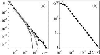
FIG. 6.: (a) Normalized distribution $p(\tau)$ in the conductive regime ($\nu$ = 60 Hz) obtained from simulations with very small lower cutoff at $U_{c}$ (full squares), and slightly above: $\Delta U=0.05$ V (squares) and $\Delta U=0.2$ V (triangles). The lines indicate the modified power law mentioned in the text. (b) shows the mean value of duration of laminar periods $\bar{\tau}$ as function of $\Delta U$. $k_{x}$ as in Fig. 4.

To distinguish between effects due to thermal fluctuations and due to a deviation from the stability threshold $\Delta U=U-U_{c}$ we have also performed simulations with $\psi_{\text{min}}=10^{-300}\psi_{\text{lam}}$ (which is obviously too small for comparison with experiment). At $U_{c}$ the power law holds now over 8 decades. Above threshold the results agree very well with $p\sim\tau^{-3/2}\exp(-$const$\,\Delta U^{2}\tau)$, see Fig. 6a. The mean duration of laminar periods behaves like $\bar{\tau}\sim\Delta U^{-1}$, cf. Fig. 6b. Similar laws have been obtained analytically in [2] for a one-dimensional mapping.

We have found on-off intermittency in a spatially extended dissipative system driven by multiplicative noise at parameter values where the first instability is towards spatially regular structures. If the strength of the noise approaches a critical value both experiment and simulations of the electrohydrodynamic equations lead to a power law with exponent $-3/2$ for the distribution of laminar periods. The simulations show that this critical value is just the threshold of stability according to the sample stability criterion [18].

This study was supported by the DFG with Grants BE 1417/3 and STA 425/3. We acknowledge valuable discussions with Prof. Agnes Buka and Heidrun Schüring.

REFERENCES

- [1] H. Fujisaka and T. Yamada, Progr. Theor. Phys. 74, 918 (1985); ibid. 75, 1087 (1986); T. Yamada and H. Fujisaka, ibid. 76, 582 (1986).
- [2] N. Platt, E. A. Spiegel, and C. Tresser, Phys. Rev. Lett. 70, 279 (1993); J. F. Heagy, N. Platt, and S. M. Hammel, Phys. Rev. E 49, 1140 (1994).
- [3] H. Fujisaka, S. Matsushita, T. Yamada, and H. Tominaga, Physics Reports 290, 27 (1997).
- [4] H. L. Yang and E. J. Ding, Phys. Rev. E 50, R3295 (1994); Z. Qu, F. Xie, and G. Hu, ibid. 53, R1301 (1996); F. Xie and G. Hu, ibid. 53, 4439 (1996); H. L. Yang, Z. Q. Huang, and E. J. Ding, ibid. 54, 3531 (1996); W. Yang, E. J. Ding, M. Ding, Phys. Rev. Lett. 76, 1808 (1996); N. Platt and S. M. Hammel, Physica A 239, 296 (1997).
- [5] H. Fujisaka, K. Ouchi, H. Hata, B. Masaoka, and S. Miyazaki, Physica D 114, 237 (1998).
- [6] K. Fukushima and T. Yamada, Phys. Lett. A 237, 141 (1998).
- [7] T. Yamada, K. Fukushima, and T. Yazaki, Progr. Theor. Phys. Suppl. 99, 120 (1989); P. W. Hammer, N. Platt, S. M. Hammel, J. F. Heagy, and B. D. Lee, Phys. Rev. Lett. 73, 1095 (1994); Y. H. Yu, K. Kwak, and T. K. Lim, Phys. Lett. A 198, 34 (1995); A. Čenys, A. Namajun̄as, A. Tamiševičius, and T. Schneider, Phys. Lett. A 213, 259 (1996); Y. Y. Hun, D. C. Kim, K. Kwak, T. K. Lim, W. Jung, Phys. Lett. A 247, 70 (1998).
- [8] F. Rödelsperger, A. Čenys, and H. Benner, Phys. Rev. Lett. 75, 2594 (1995).
- [9] M. Sauer and F. Kaiser, Phys. Rev. E 54, 2468 (1996).
- [10] D. L. Feng, C. X. Yu, J. L. Xie, and W. X. Ding, Phys. Rev. E 58, 3678 (1998).
- [11] L. Kramer and W. Pesch, Annu. Rev. Fluid Mech. 17, 515 (1995); in: Pattern Formation in Liquid Crystals, edited by A. Buka and L. Kramer, (Springer, New York, 1995) pp. 69-90; W. Pesch and U. Behn, in Evolution of Spontaneous Structures in Dissipative Continuous Systems, edited by F. H. Busse and S. C. Müller (Springer, Heidelberg, 1998) pp. 335-383.
- [12] S. Kai, T. Kai, M. Takata, and K. Hirakawa, J. Phys. Soc. Jpn. 47, 1379 (1979); T. Kawakubo, A. Yanagita, and S. Kabashima, J. Phys. Soc. Jpn. 50, 1451 (1981).
- [13] H. R. Brand, S. Kai, and S. Wakabayashi, Phys. Rev. Lett. 54, 555 (1985); S. Kai, T. Tamura, S. Wakabayashi, M. Imasaki, and H. R. Brand, IEEE-IAS Conf. Records 85CH, 1555 (1985).
- [14] S. Kai, H. Fukunaga, and H. R. Brand, J. Phys. Soc. Jpn. 56, 3759 (1987); J. Stat. Phys. 54, 1133 (1989).
- [15] S. Kai, in: Noise in nonlinear dynamical systems, edited by F. Moss and P. V. E. McClintock (Cambridge University Press, Cambridge, 1989) pp. 22-76; H. R. Brand, ibid. pp. 77-89.
- [16] H. Amm, U. Behn, Th. John, and R. Stannarius, Mol. Cryst. Liq. Cryst. 304, 525 (1997).
- [17] U. Behn and R. Müller, Phys. Lett. 113A, 85 (1985); R. Müller and U. Behn, Z. Phys. B 69, 185 (1987); ibid. 78, 229 (1990); A. Lange, R. Müller, and U. Behn, ibid. 100, 447 (1996).
- [18] U. Behn, A. Lange, and Th. John, Phys. Rev. E 58, 2047 (1998).