Existence and stability of hole solutions to complex Ginzburg-Landau equations

Abstract

We consider the existence and stability of the hole, or dark soliton, solution to a Ginzburg-Landau perturbation of the defocusing nonlinear Schrödinger equation (NLS), and to the nearly real complex Ginzburg-Landau equation (CGL). By using dynamical systems techniques, it is shown that the dark soliton can persist as either a regular perturbation or a singular perturbation of that which exists for the NLS. When considering the stability of the soliton, a major difficulty which must be overcome is that eigenvalues may bifurcate out of the continuous spectrum, i.e., an edge bifurcation may occur. Since the continuous spectrum for the NLS covers the imaginary axis, and since for the CGL it touches the origin, such a bifurcation may lead to an unstable wave. An additional important consideration is that an edge bifurcation can happen even if there are no eigenvalues embedded in the continuous spectrum. Building on and refining ideas first presented in Kapitula and Sandstede [35] and Kapitula [32], we show that when the wave persists as a regular perturbation, at most three eigenvalues will bifurcate out of the continuous spectrum. Furthermore, we precisely track these bifurcating eigenvalues, and thus are able to give conditions for which the perturbed wave will be stable. For the NLS the results are an improvement and refinement of previous work, while the results for the CGL are new. The techniques presented are very general and are therefore applicable to a much larger class of problems than those considered here.

AMS classification scheme numbers: 30B10, 30B40, 34A05, 34A26, 34A47, 34C35, 34C37, 34D15, 34E05, 35K57, 35P15, 35Q51, 35Q55, 78A60

1 Introduction

The standard model for the propagation of pulses in an ideal defocussing nonlinear fiber without loss is the cubic nonlinear Schrödinger equation (NLS)

$$i\phi_{t}-\frac{1}{2}\phi_{xx}-\phi+|\phi|^{2}\phi=0,$$ (1.1)

for $x\in{\rm I\kern-2.29996ptR}$. It supports the dark soliton solution, which is given by

$$\Phi(x)=\tanh(x).$$ (1.2)

If loss is present in the fiber, then the dark soliton will cease to exist. Thus, at a minimum amplifiers must be used to compensate for the loss. The effects of linear loss in the fiber as well as linear and nonlinear amplification of the wave along the fiber will be incorporated into the model. The issues to be discussed in this paper are the persistence of the dark soliton under perturbation, and the stability of the persisting solution relative to the PDE. In this article, we shall concentrate on these issues for a particular perturbation. We emphasize, however, that the methods and ideas presented herein are general, and they are applicable to a much larger class of problems. Here we will consider a perturbed NLS (PNLS) which is given by

$$i\phi_{t}-\frac{1}{2}\phi_{xx}-\phi+|\phi|^{2}\phi=i\epsilon(\frac{1}{2}d_{1}\phi_{xx}+d_{2}\phi+d_{3}|\phi|^{2}\phi+d_{4}|\phi|^{4}\phi),$$ (1.3)

where $\epsilon>0$ is small and the other parameters are real and of $O(1)$ in $\epsilon$. The nonnegative parameter $d_{1}$ describes spectral filtering, $d_{2}$ describes the linear gain ($d_{2}>0$) or loss ($d_{2}<0$) due to the fiber, and $d_{3}$ and $d_{4}$ describe the nonlinear gain or loss due to the fiber.

A related equation is the nearly real complex Ginzburg-Landau equation (CGL)

$$\phi_{t}-\frac{1}{2}\phi_{xx}-\phi+|\phi|^{2}\phi=i\epsilon(\frac{1}{2}d_{1}\phi_{xx}+d_{2}\phi+d_{3}|\phi|^{2}\phi+d_{4}|\phi|^{4}\phi),$$ (1.4)

where again $\epsilon>0$ is small and the other parameters are real and of $O(1)$. The CGL governs the nonlinear evolution of perturbations of a simple solution of a basic system of partial differential equations at near critical conditions, provided that the basic system satisfies some generic conditions (Eckhaus [14]). The CGL has been proven valid in an asymptotic sense for a large class of systems (Collet and Eckmann [7], van Harten [20], Bollerman et al [2], Mielke and Schneider [40], and Schneider [46, 47]). The CGL results from an asymptotic expansion, and equation (1.4) with $d_{4}=0$ is only the $O(1)$ part of a more extended equation. The inclusion of the $d_{4}$ term is a means of modelling the effect of small, nonlinear higher order corrections (Doelman [10], Popp et al [41], Stiller et al [49, 50]).

It is clear that studying the existence of steady-state solutions to equations (1.3) and (1.4) amounts to determining the solution structure for the equation

$$-\frac{1}{2}\phi^{\prime\prime}-\phi+|\phi|^{2}\phi=i\epsilon(\frac{1}{2}d_{1}\phi^{\prime\prime}+d_{2}\phi+d_{3}|\phi|^{2}\phi+d_{4}|\phi|^{4}\phi)$$ (1.5)

(${}^{\prime}=\frac{d}{dx}$). To do this, one can set

• $\displaystyle\hskip 60.0pt{\phi(x)=r(x)e^{i\int_{0}^{x}\psi(s)\,ds},}$

and then study trajectories in the $(r,r^{\prime},\psi)$ phase space. This task has been done in a series of papers, of which Doelman and Doelman et al [8, 9, 10, 11], Duan et al [13], Holmes [21], Jones et al [26], Kapitula and Kapitula et al [29, 31, 33], Marcq et al [38], and Van Saarloos et al [44] are a sample. In Section 2 we prove the following theorem regarding the persistence of the wave given by (1.2). The result is not entirely new, as it is alluded to by Doelman [10]. To determine the stability of the perturbed waves relative to the PDEs, however, we need more detailed asymptotic information than that which is provided in [10].

Theorem 1.1

Suppose that

• $\displaystyle\hskip 60.0pt{d_{2}+d_{3}+d_{4}=-\epsilon^{2}\sigma^{*}(\epsilon)-\sigma,}$

where

• $\displaystyle\hskip 60.0pt{\sigma^{*}(0)=-\frac{2}{9}(d_{1}+d_{3}+\frac{8}{5}d_{4})^{2}(d_{1}+d_{3}+2d_{4}).}$

Suppose that $(\epsilon^{2}\sigma^{*}(\epsilon)+\sigma)(d_{1}+d_{3}+2d_{4})<0$. If $\sigma=0$, then the wave persists as a regular perturbation, with the asymptotic expansion

• $\displaystyle\hskip 60.0pt{\begin{array}[]{lll}r(x)&=&\Phi(x)+O(\epsilon^{2})\\ \vspace{.1mm}\\ \psi(x)&=&{\displaystyle\frac{2}{3}\left((d_{1}+d_{3}+d_{4})\Phi(x)+\frac{3}{5}d_{4}\Phi^{3}(x)\right)\epsilon+O(\epsilon^{3})}.\end{array}}$

If $\sigma\neq 0$, then the wave persists as a singular perturbation.

Remark 1.2

When $\sigma\neq 0$, the radial profile of the wave will have a “shelf” ([4, 5, 22, 23]).

Remark 1.3

The wave $-\Phi$, which exists for $\epsilon=0$, persists under the same conditions; our analysis shows that it has the same stability characteristics as $\Phi$ as well. For concreteness, we will simply refer to $\Phi$ throughout this paper.

It seems that all previous attempts to consider the stability of the wave, especially for the PNLS, have ignored the fact that the wave persists as a singular perturbation except on the regular perturbation manifold $d_{2}+d_{3}+d_{4}=-\epsilon^{2}\sigma^{*}$; relevant works include Burtsev et al [4], Chen et al [5], Ikeda et al [22, 23], and Lega et al [36]. If the parameters do not lie on the regular perturbation manifold, then it may be the case that the “shelf” can influence the stability of the wave. One possible way of attacking this problem may be through the topological methods first introduced by Jones [24] and Alexander et al [1], and later used in a variety of contexts by, for example, Bose et al [3], Doelman et al [12], Gardner and Gardner et al [16, 17, 18], and Rubin and Rubin et al [42, 43]. This issue will not be addressed in this paper and will be a topic of future study.

Here, we suppose that the wave does persist as a regular perturbation. Since the equations under consideration are posed on the unbounded real line, the spectrum of the linearization about the wave contains continuous spectrum corresponding to radiation modes. In addition, the spectrum may contain several isolated eigenvalues of finite multiplicity. Because of the translation and rotation invariance of the PNLS and CGL, zero is an eigenvalue. It is not, however, an isolated eigenvalue. When $\epsilon=0$, the continuous spectrum for the NLS covers the imaginary axis, while that for the CGL covers the negative real axis. Furthermore, there are no point eigenvalues in the open right-half plane for either equation. For $\epsilon\neq 0$, the origin is still contained in the continuous spectrum. By choosing the parameters appropriately, one can bound the continuous spectrum in the closed left-half plane. To determine the stability of the wave for $\epsilon\neq 0$, it is thus necessary to locate the point eigenvalues. There are standard tools available which can be used to determine the fate of isolated eigenvalues (see, for example, Kapitula [32]). However, it is a difficult and nonstandard problem to determine the conditions under which eigenvalues can bifurcate out of the continuous spectrum, i.e., conditions under which an edge bifurcation can occur. The primary issue of this paper is the detection of such eigenvalues. We emphasize that an edge bifurcation may occur even if the corresponding eigenfunctions in the unperturbed problem are not localized.

We now turn to an outline of our approach for locating eigenvalues. In many respects it follows that presented in Kapitula et al [35], which deals with the stability of solitary wave solutions for the focusing NLS. The major tool that we use is the Evans function, $E(\lambda)$. The Evans function is a complex-valued function depending on $\lambda\in{\mathchoice{\hbox{\hbox to0.0pt{\kern 2.88884pt\vrule height=6.49162pt\hss}\hbox{$\displaystyle\rm C$}}}{\hbox{\hbox to0.0pt{\kern 2.88884pt\vrule height=6.49162pt\hss}\hbox{$\textstyle\rm C$}}}{\hbox{\hbox to0.0pt{\kern 2.02219pt\vrule height=4.54414pt\hss}\hbox{$\scriptstyle\rm C$}}}{\hbox{\hbox to0.0pt{\kern 1.44441pt\vrule height=3.2458pt\hss}\hbox{$\scriptscriptstyle\rm C$}}}}$ with the property that $E(\lambda)=0$ whenever $\lambda$ is an isolated eigenvalue. It is only defined a-priori away from the continuous spectrum, so it is not immediately clear that it can be used to locate embedded eigenvalues and detect edge bifurcations. However, as an application of the Gap Lemma, discovered simultaneously and independently by Kapitula et al [35] and Gardner et al [19], the Evans function can be analytically extended across the continuous spectrum. The analytic extension can then in theory be used to locate embedded eigenvalues and to track them under perturbation.

In the problems considered so far, it turns out that the continuous spectrum corresponds to a branch cut for the Evans function. Furthermore, in these problems it is only at the branch point that the Evans function has an embedded zero, so only from there can an eigenvalue bifurcate. For the problems under consideration both in this paper and in Kapitula et al [35], when $\epsilon=0$ the edge of the continuous spectrum is a branch point of order one, i.e., near the edge of the continuous spectrum we can write $E(\lambda)=f(\sqrt{\lambda-\lambda_{b}})$, where $f(\cdot)$ is analytic and $\lambda_{b}$ is the branch point. In [35] the stability of the solitary wave to the perturbed focusing NLS was considered. It turned out that for a suitably scaled eigenvalue parameter that near the branch point $\lambda_{b}=i\omega$ the Evans function could be written as

• $\displaystyle\hskip 60.0pt{E(\lambda,\epsilon)=\sqrt{\lambda-i\omega}+A\epsilon,}$

where $A\in{\mathchoice{\hbox{\hbox to0.0pt{\kern 2.88884pt\vrule height=6.49162pt\hss}\hbox{$\displaystyle\rm C$}}}{\hbox{\hbox to0.0pt{\kern 2.88884pt\vrule height=6.49162pt\hss}\hbox{$\textstyle\rm C$}}}{\hbox{\hbox to0.0pt{\kern 2.02219pt\vrule height=4.54414pt\hss}\hbox{$\scriptstyle\rm C$}}}{\hbox{\hbox to0.0pt{\kern 1.44441pt\vrule height=3.2458pt\hss}\hbox{$\scriptscriptstyle\rm C$}}}}$ depended upon the particular perturbation. Thus, for that problem at most one eigenvalue could pop out of the continuous spectrum.

To determine the location of the zeros of $E(\lambda)$ near $\lambda_{b}$ for those problems in which more than one eigenvalue can pop out of the continuous spectrum, one would like to write the Evans function as the series

• $\displaystyle\hskip 60.0pt{E(\gamma)=\sum_{n=0}^{\infty}a_{n}\gamma^{n},\quad\gamma^{2}=\lambda-\lambda_{b},}$

and then locate its zeros. This task can be accomplished if one can derive asymptotic expressions for the coefficients of the series. Fortunately, by suitably modifying the ideas and methods of Kapitula [32], which were developed for doing Taylor expansions around isolated eigenvalues, we are able to derive such expressions. Once the zeros of the expansion have been located, we take those zeros that lie on the correct sheet of the appropriate Riemann surface and invert to find the eigenvalues for the system. The interested reader should consult Section 3 for more details.

It turns out, for both the PNLS and the CGL, that when $\epsilon=0$ the Evans function has a branch point at $\lambda=0$ and is nonzero everywhere else in the closed right-half plane. Furthermore, when $\epsilon=0$ the Evans function has the expansion

• $\displaystyle\hskip 60.0pt{E(\gamma)=A\gamma^{3}+O(\gamma^{4}),}$

where $A\in{\rm I\kern-2.29996ptR}$ and $\gamma$ is a suitably defined function of $\lambda$ for $\lambda$ near zero (see Section 3 for details). Thus, for the perturbed problem, there will be three zeros of the Evans function near $\gamma=0$, and hence there will be at most three eigenvalues in this region. By computing the lower order terms in the series, we are able to locate these eigenvalues and assess the stability of the hole solution. As the following theorem illustrates, for the PNLS there are at most two eigenvalues which bifurcate out of the branch point $\lambda=0$ and leave the continuous spectrum. Furthermore, the $d_{4}$ term must be nonzero (specifically, negative) for the wave to be linearly stable.

Theorem 1.4

Suppose that $d_{2}+d_{3}+d_{4}=-\epsilon^{2}\sigma^{*}(\epsilon)$, where $\sigma^{*}$ is given in Theorem 1.1. Also, assume that $d_{3}+2d_{4}<0$.

  i)

Suppose that $d_{1}>0$, and set $P_{j1}=d_{j}/d_{1}$. If

• $\displaystyle\hskip 60.0pt{P_{31}<-\frac{4}{5}P_{41}-1,}$

then the linearization of (1.3) about the perturbed wave yields a positive $O(\epsilon)$ real eigenvalue given to leading order by

• $\displaystyle\hskip 60.0pt{\lambda_{1}=-(d_{3}+2d_{4})\left(\sqrt{1+\frac{4}{9}\frac{(1+P_{31}+4P_{41}/5)^{2}}{(P_{31}+2P_{41})^{2}}}-1\right)\,\epsilon.}$

Furthermore, if

• $\displaystyle\hskip 60.0pt{P_{31}>-\frac{8}{5}P_{41}-1,\quad P_{31}>-2P_{41}-\frac{5}{4},}$

then there is a positive $O(\epsilon^{3})$ real eigenvalue which is given to leading order by

• $\displaystyle\hskip 60.0pt{\lambda_{2}=-\frac{\tilde{\gamma}}{2(P_{31}+2P_{41})}\epsilon^{3},}$

where

• $\displaystyle\hskip 60.0pt{\tilde{\gamma}=\frac{4}{9}d_{1}^{3}(1+P_{31}+\frac{8}{5}P_{41})^{2}(\frac{5}{4}+P_{31}+2P_{41}).}$

Otherwise, the wave is linearly stable, as no other eigenvalues bifurcate from the continuous spectrum (see Figure 1).

  ii)

If $d_{1}=0$, then the wave is linearly stable as a solution of (1.3) if $5d_{3}+4d_{4}<0$; otherwise, there is an $O(\epsilon)$ eigenvalue which is given to leading order by

• $\displaystyle\hskip 60.0pt{\lambda_{1}=-(d_{3}+2d_{4})\left(\sqrt{1+\frac{4}{9}\frac{(d_{3}+4d_{4}/5)^{2}}{(d_{3}+2d_{4})^{2}}}-1\right)\,\epsilon.}$

Remark 1.5

The condition that $d_{1}\geq 0$ and $d_{3}+2d_{4}<0$ ensures that the continuous spectrum is contained in the closed left-half plane for $\epsilon>0$ and small.

Remark 1.6

If $d_{4}=0$ the wave is linearly unstable, with an $O(\epsilon)$ eigenvalue if $P_{31}<-1$ and an $O(\epsilon^{3})$ eigenvalue if $-1<P_{31}<0$. Furthermore, the wave is linearly unstable if $d_{4}>0$.

Before we discuss the stability of the wave for the CGL, a few comments are in order. There have been many recent efforts to determine the stability of the dark soliton for the perturbed NLS by using an adiabatic approach ([4, 5, 22, 23, 36]). With the adiabatic approach the wave is predicted to be stable if both $d_{3}+2d_{4}<0$ and $d_{1}+d_{3}+6d_{4}/5>0$ hold. If $d_{4}=0$, then this approach is consistent with the result of Theorem 1.4 in that it correctly determines the stability of the wave up to $O(\epsilon)$. However, it does not predict the existence of the $O(\epsilon^{3})$ instability; this is not surprising, as the adiabatic approach is only meant to understand the dynamics on a time scale of $O(1/\epsilon)$. If $d_{4}\neq 0$, then the analysis contradicts the results presented in this paper, even at the $O(\epsilon)$ level. This contradiction implies that the original adiabatic ansatz for the slow-time variation of the wave is incorrect (see Section 5.5 for more details). In some way the parameter $d_{4}$ has the same effect on the stability analysis for the perturbed wave as it has on the solution structure for the steady-state problem, i.e., it breaks some kind of “hidden symmetry” (see Doelman [10]). This topic would be an interesting avenue for further research.

When considering the stability of the wave to the CGL, the primary difficulty is that the resulting Evans function is not as easy to factor as that associated with the PNLS. As such, for general parameter values the location of bifurcating eigenvalues cannot be put into an easily readable form. However, one can determine for which ranges in the parameter space there will be eigenvalues with positive real part; as with the PNLS, it turns out that at most two eigenvalues bifurcate from the continuous spectrum. As it can be seen from the following theorem, a primary difference between the PNLS and the CGL when considering the stability of the hole solution is the order of the eigenvalues. In general, the instability will grow much more slowly for the CGL than for the PNLS.

Theorem 1.7

Suppose that $d_{2}+d_{3}+d_{4}=-\epsilon^{2}\sigma^{*}(\epsilon)$, where $\sigma^{*}$ is given in Theorem 1.1. Set

• $\displaystyle\hskip 60.0pt{\mu_{sn}^{\pm}=\frac{3}{2}\frac{\pm\alpha-2/3}{1\mp\alpha},\quad\alpha^{2}=\frac{\sqrt{125}+11}{2}}$

($\mu_{sn}^{+}=-1.716,\,\mu_{sn}^{-}=-1.385$).

  i)

Suppose that $d_{1}\neq 0$, and set $P_{j1}=d_{j}/d_{1}$. If

• $\displaystyle\hskip 60.0pt{(\frac{3}{2}+P_{31}+2P_{41})(1+P_{31}+\frac{8}{5}P_{41})<0,}$

then there is one positive real $O(\epsilon^{4})$ eigenvalue for the linearized problem, and the wave is linearly unstable. If

• $\displaystyle\hskip 60.0pt{d_{1}(1+P_{31}+\frac{8}{5}P_{41})>0,\quad d_{1}(\mu_{sn}^{-}+P_{31}+2P_{41})>0}$

or

• $\displaystyle\hskip 60.0pt{d_{1}(1+P_{31}+\frac{8}{5}P_{41})<0,\quad d_{1}(\mu_{sn}^{+}+P_{31}+2P_{41})<0,}$

then there is a complex pair of $O(\epsilon^{4})$ eigenvalues with negative real part. Otherwise, no eigenvalues bifurcate from the continuous spectrum (see Figure 2). In either case, if

• $\displaystyle\hskip 60.0pt{(\frac{3}{2}+P_{31}+2P_{41})(1+P_{31}+\frac{8}{5}P_{41})>0,}$

then the wave is linearly stable.

  ii)

Suppose that $d_{1}=0$ and set

• $\displaystyle\hskip 60.0pt{a=(d_{3}+2d_{4})(d_{3}+\frac{8}{5}d_{4}).}$

If $a>0$, then the zeros of the Evans function inside the curve $K$ are given by

• $\displaystyle\hskip 60.0pt{\lambda_{2,3}=(-0.595\pm 0.255i)\,a^{2}\epsilon^{4},}$

and the wave is linearly stable as a solution of (1.4). If $a<0$, then the zero of the Evans function inside $K$ is given by

• $\displaystyle\hskip 60.0pt{\lambda_{1}=1.191\,a^{2}\epsilon^{4},}$

and the wave is linearly unstable.

Remark 1.8

The continuous spectrum remains in the closed left-half plane for all values of $d_{1},\dots,d_{4}$ as long as $\epsilon>0$ is sufficiently small.

Remark 1.9

The sign of the parameter $a$ corresponds to the manner in which the wave is constructed in the $(r,r^{\prime},\psi)$ phase space. The interested reader should consult Section 2 for more details.

Remark 1.10

If $d_{1}\neq 0$, it may be the case that there is a complex pair of eigenvalues with negative real part. The interested reader should consult Lemma 4.8 for the details.

The remainder of this paper is organized in the following manner. In Section 2 the conditions for the persistence of the wave are derived through the use of dynamical systems techniques. In Section 3 we derive the expressions which allow us to compute Taylor expansions at the branch point of the Evans function. This section is relatively self-contained and can be skipped on a first reading. In Sections 4 and 5 we calculate the Taylor expansion for the Evans function for the CGL and the PNLS, respectively. Theorem 1.7 follows from Lemmas 4.6 and 4.8. Theorem 1.4 follows from Lemma 5.6. Section 5 concludes with a brief discussion comparing the approach of this paper with the previous adiabatic approaches.

Remark 1.11

Recently, Li and Promislow [37] independently and simultaneously used some of the ideas present in this paper to study the stability of waves to the equations describing pulse propagation in linearly birefringent, lossless fibers.

2 Existence and persistence

The steady-state problem for both the PNLS and the CGL is given by

$$-\frac{1}{2}\phi^{\prime\prime}-\phi+|\phi|^{2}\phi=i\epsilon(\frac{1}{2}d_{1}\phi^{\prime\prime}+d_{2}\phi+d_{3}|\phi|^{2}\phi+d_{4}|\phi|^{4}\phi)$$ (2.1)

(${}^{\prime}=\frac{d}{dx}$). For existence of the hole solution, which is given by

$$\Phi(x)=\tanh x$$ (2.2)

when $\epsilon=0$, we will want to consider the problem in polar coordinates. Set

$$\phi(x)=r(x)e^{i\int_{0}^{x}\psi(s)\,ds}$$ (2.3)

to obtain (after dropping higher order terms that do not affect subsequent calculations) the three-dimensional system of ODEs

$$\begin{array}[]{rll}r^{\prime}&=&s\\ s^{\prime}&=&-2r(1-r^{2})+r\psi^{2}\\ &&\quad-2\epsilon^{2}d_{1}r(d_{2}-d_{1}+(d_{1}+d_{3})r^{2}+d_{4}r^{4})\\ \psi^{\prime}&=&-2\frac{s}{r}\psi-2\epsilon(d_{2}-d_{1}+(d_{1}+d_{3})r^{2}+d_{4}r^{4}).\end{array}$$ (2.4)

For the system (2.4) there exist are two critical manifolds ${\cal M}_{\epsilon}^{\pm}$, which when $\epsilon=0$ are given by

$${\cal M}^{\pm}_{0}=\{(r,s,\psi)\,:\,r=\pm\sqrt{1-\psi^{2}/2},\,\psi^{2}<2/3\};$$ (2.5)

we restrict to $\psi^{2}<2/3$ in (2.5) so that the manifolds ${\cal M}_{\epsilon}^{\pm}$ are normally hyperbolic. Each critical manifold of (2.4) has a two-dimensional unstable manifold, $W^{u}({\cal M}^{\pm}_{\epsilon})$, and a two-dimensional stable manifold, $W^{s}({\cal M}^{\pm}_{\epsilon})$, which are smooth perturbations of the center-stable and center-unstable manifolds which exist when $\epsilon=0$ [15, 25]. As it will be seen, it can be shown that $W^{u}({\cal M}^{-}_{\epsilon})\cap W^{s}({\cal M}^{+}_{\epsilon})\neq\emptyset$, and, by the symmetry $(r,s,\psi,x)\to(r,-s,-\psi,-x),\,W^{u}({\cal M}^{+}_{\epsilon})\cap W^{s}({\cal M}^{-}_{\epsilon})\neq\emptyset$, both for $0\leq\epsilon<\epsilon_{0}$ for some $\epsilon_{0}>0$. These relationships are clearly satisfied when $\epsilon=0$, as evidenced by the existence of the waves $\pm\Phi$. Assuming that the relevant manifolds intersect, the wave $\Phi$ will persist as long as the parameters are chosen so that critical points exist on ${\cal M}^{\pm}_{\epsilon}$ (also see Doelman [8, 9]). Depending how the parameters are chosen, there will be zero, two, or four critical points on ${\cal M}^{\pm}_{\epsilon}$ (counting multiplicities). The condition $\psi^{2}<2/3$ implies that the critical points on ${\cal M}^{\pm}_{\epsilon}$ correspond to stable periodic solutions to (2.1) [28, 30].

To prove the existence of multiple orbits bifurcating from the original heteroclinic cycle with the constraint that the orbits remain within an small tube of the original cycle, it will be useful to set

$$d_{2}+d_{3}+d_{4}=-(\epsilon^{2}\sigma^{*}+\sigma),$$ (2.6)

where $\sigma^{*}(\epsilon)$ is such that

$$\sigma^{*}(0)=-\frac{2}{9}(d_{1}+d_{3}+\frac{8}{5}d_{4})^{2}(d_{1}+d_{3}+2d_{4}),$$ (2.7)

as in the statement of Theorem 1.1. It will henceforth be assumed that the parameter $\sigma$, while small, is independent of $\epsilon$.

Remark 2.1

Equation (2.6) is not a parameter restriction for the CGL, as it can always be achieved by going into an appropriate rotating reference frame. However, it is a restriction for the PNLS, and determines a balance between the linear loss and nonlinear gain.

Substituting relation (2.6) into the ODE (2.4) yields

$$\begin{array}[]{rll}r^{\prime}&=&s\\ s^{\prime}&=&-2r(1-r^{2})+r\psi^{2}\\ &&\quad+2\epsilon^{2}d_{1}r[(d_{1}+d_{3})(1-r^{2})+d_{4}(1-r^{4})+\epsilon^{2}\sigma^{*}+\sigma]\\ \psi^{\prime}&=&-2\frac{s}{r}\psi+2\epsilon[(d_{1}+d_{3})(1-r^{2})+d_{4}(1-r^{4})+\epsilon^{2}\sigma^{*}+\sigma].\end{array}$$ (2.8)

Since the lowest order at which $\sigma$ appears in (2.8) is at $O(\epsilon)$ in the $\psi$-equation, the effect of $\sigma$ on perturbation calculations will only be felt at $O(\epsilon+\sigma)\epsilon$, except in terms of the location of critical points on ${\cal M}_{\epsilon}$, which is discussed below. Hence, for many of the perturbation calculations that follow, the role of $\sigma$ can be ignored.

The following two propositions detail the relevant behavior on ${\cal M}^{\pm}_{\epsilon}$. The proofs can be found in Kapitula [31] and hence are omitted.

Proposition 2.2

Suppose that $d_{2}+d_{3}+d_{4}=-(\epsilon^{2}\sigma^{*}+\sigma)$ and that

• $\displaystyle\hskip 60.0pt{(\epsilon^{2}\sigma^{*}+\sigma)(d_{1}+d_{3}+2d_{4})<0.}$

Then a pair of critical points on ${\cal M}^{+}_{\epsilon}$ [${\cal M}^{-}_{\epsilon}$] are given by $(r^{*}_{+},0,\pm\psi^{*})$ [$(r^{*}_{-},0,\pm\psi^{*})$], where

• $\displaystyle\hskip 60.0pt{\begin{array}[]{lll}{\displaystyle r^{*}_{\pm}}&=&{\pm\left(\displaystyle 1+\frac{1}{2}\frac{\epsilon^{2}\sigma^{*}+\sigma}{d_{1}+d_{3}+2d_{4}}\right)}\\ \vspace{.1mm}\\ \psi^{*}&=&{\displaystyle\sqrt{-2\frac{\epsilon^{2}\sigma^{*}+\sigma}{d_{1}+d_{3}+2d_{4}}}}.\end{array}}$

Proposition 2.3

When $0\leq\epsilon\ll 1$, the manifolds ${\cal M}^{\pm}_{\epsilon}$ intersect the $r$-axis. Further, there exists $\delta$, with $1\gg\delta>0$, such that for $-(\psi^{*}+\delta)<\psi<\psi^{*}+\delta$ the flow on ${\cal M}^{\pm}_{\epsilon}$ is given by

• $\displaystyle\hskip 60.0pt{\psi^{\prime}=\epsilon((d_{1}+d_{3}+2d_{4})\psi^{2}+2\epsilon^{2}\sigma^{*}+2\sigma).}$

Proposition 2.2 gives a condition for the existence of critical points on ${\cal M}^{+}_{\epsilon}$. It remains to show that $W^{u}({\cal M}^{-}_{\epsilon})\cap W^{s}({\cal M}^{+}_{\epsilon})\neq\emptyset$ for small $\epsilon\neq 0$. Let $\Sigma_{o}^{p}=\{(r,s,\psi):r=\psi=0\}$. The hole solution belongs to $\Sigma_{o}^{p}$ at $x=0$, with $s(0)\neq 0$. When $\epsilon=0$, the manifold $W^{s}({\cal M}^{+}_{\epsilon})$ intersects the curve $\Sigma_{o}^{p}$ transversely in $(r,s,\psi)$-space, since $W^{s}({\cal M}^{+}_{0})$ is transverse to the invariant $\{\psi=0\}$ plane. Thus, the intersection will persist for $\epsilon\neq 0$ sufficiently small. Due to invariance under $(r,s,\psi,x)\to(-r,s,-\psi,-x)$ and the fact that $s(0)\neq 0$ along the $\epsilon=0$ solution, it can then be concluded that not only does $W^{u}({\cal M}^{-}_{\epsilon})$ also intersect $\Sigma_{o}^{p}$ transversely, but $W^{u}({\cal M}^{-}_{\epsilon})\cap W^{s}({\cal M}^{+}_{\epsilon})\neq\emptyset$ as well. Hence, the hole solution will persist for $\epsilon\neq 0$ and small. The result is not new (for example, see Doelman [8]). To determine the stability of the wave, however, more information about the wave must be known than has previously been given.

In the remainder of this section, we finish the proof of Theorem (1.1) by showing that for $\sigma=0$ the perturbed wave arises as a regular perturbation, and then compute its asymptotics. We conclude with a discussion of how the nature of the intersection that yields the wave differs in various parameter regimes; this is where Proposition 2.3 is useful.

Let an underlying hole solution be denoted by $(R,S,\Psi)$. When evaluated at $\epsilon=\sigma=0$, the variational equations associated with (2.8) are given by

$$\begin{array}[]{lll}\delta r^{\prime}&=&\delta s\\ \delta s^{\prime}&=&-2(1-3R^{2}-\Psi^{2}/2)\,\delta r+2R\Psi\,\delta\psi\\ \delta\psi^{\prime}&=&2R^{\prime}\Psi/R^{2}\,\delta r-2\Psi/R\,\delta s-2R^{\prime}/R\,\delta\psi\\ &{}&\quad\quad+2[(d_{1}+d_{3})(1-R^{2})+d_{4}(1-R^{4})]\,\delta\epsilon\\ \delta\epsilon^{\prime}&=&0\\ \delta\sigma^{\prime}&=&0.\end{array}$$ (2.9)

Since the solution belongs to $\Sigma_{o}^{p}$ at $x=0$ even for $\epsilon\neq 0$, it is of interest to determine the location of the curve $\Sigma_{o}^{p}$ as the flow carries it up to the slow manifold ${\cal M}^{+}_{\epsilon}$. Specifically, we wish to determine the $\psi$-coordinates of the points of $\Sigma_{o}^{p}$ as they approach ${\cal M}^{+}_{\epsilon}$. Using the fact that the $\psi$-coordinate of $\Sigma_{o}^{p}$ is identically zero when $\epsilon=0$, by doing a Taylor expansion we can write that $\psi=\psi_{\epsilon}\epsilon+O(\epsilon^{2})$. From evaluation of the variational equations over the $\epsilon=0$ hole solution $\Phi$, we find that $\psi_{\epsilon}$ satisfies the initial value problem

$$\begin{array}[]{l}{\displaystyle(\Phi^{2}\psi_{\epsilon})^{\prime}=2[(d_{1}+d_{3})(1-\Phi^{2})+d_{4}(1-\Phi^{4})]\Phi^{2}}\\ {\displaystyle(\Phi^{2}\psi_{\epsilon})(0)=0}.\end{array}$$ (2.10)

Upon integrating, it is seen that

$$\psi_{\epsilon}(x)=\frac{2}{3}\left((d_{1}+d_{3}+d_{4})\Phi(x)+\frac{3}{5}d_{4}\Phi^{3}(x)\right).$$ (2.11)

Let $0<\nu\ll 1$ be given, and let $T_{\nu}>0$ be such that $1-\Phi(T_{\nu})=\nu$. That is, $T_{\nu}$ denotes a time when the curve $\Sigma_{o}^{p}$ is within $O(\nu)$ of the slow manifold ${\cal M}^{+}_{\epsilon}$. Upon evaluating the expression for $\psi_{\epsilon}$ at $T_{\nu}$, it is seen that

$$\psi_{\epsilon}(T_{\nu})=\frac{2}{3}(d_{1}+d_{3}+\frac{8}{5}d_{4})+O(\nu).$$ (2.12)

The following proposition has now been proved.

Proposition 2.4

At the time $T_{\nu}$ such that $1-\Phi(T_{\nu})=\nu$, the image of the curve $\Sigma_{o}^{p}$ under the flow is within an $O(\nu)$ distance of the slow manifold ${\cal M}^{+}_{\epsilon}$, and the $\psi$-coordinates of points on the image of $\Sigma_{o}^{p}$ are given by

• $\displaystyle\hskip 60.0pt{\psi=[\frac{2}{3}(d_{1}+d_{3}+\frac{8}{5}d_{4})+O(\nu)]\epsilon+O(\epsilon+\sigma)\epsilon,}$

where $0<\epsilon,\nu\ll 1$.

First suppose that $\sigma=0$. As a consequence of the manner in which $\sigma^{*}$ has been chosen, an application of Propositions 2.2 and 2.4 yields that the wave will persist as a regular perturbation. This is due to the fact that the critical points on ${\cal M}^{+}_{\epsilon}$ match the expression given in Proposition 2.4. The following lemma gives the necessary asymptotics for the perturbed wave. The proof is a standard application of perturbation theory, and hence will be left to the interested reader.

Lemma 2.5

Suppose that $\sigma=0$. The perturbed wave then arises as a regular perturbation and satisfies

• $\displaystyle\hskip 60.0pt{\begin{array}[]{lll}r&=&\Phi+r_{\epsilon\epsilon}\epsilon^{2}/2+O(\epsilon^{3})\\ \psi&=&\psi_{\epsilon}\epsilon+O(\epsilon^{3}),\end{array}}$

where

• $\displaystyle\hskip 60.0pt{\psi_{\epsilon}(x)=\frac{2}{3}\left((d_{1}+d_{3}+d_{4})\Phi(x)+\frac{3}{5}d_{4}\Phi^{3}(x)\right)}$

and

• $\displaystyle\hskip 60.0pt{\begin{array}[]{lll}r_{\epsilon\epsilon}(x)&=&{\displaystyle\frac{1}{225}[-5(10(d_{1}+d_{3})^{2}+40(d_{1}+d_{3})d_{4}+39d_{4}^{2})\Phi(x)}\\ \vspace{.1mm}\\ &&\quad+8d_{4}(5(d_{1}+d_{3})+8d_{4})\Phi^{3}(x)+3d_{4}^{2}\Phi^{5}(x)\\ \vspace{.1mm}\\ &&\quad+12d_{4}(5(d_{1}+d_{3})+8d_{4})x\Phi^{\prime}(x)]\\ \vspace{.1mm}\\ &&\quad\quad{\displaystyle+\frac{1}{3}d_{1}[2d_{4}\Phi(x)-3(d_{1}+d_{3}+2d_{4})x\Phi^{\prime}(x)]\Phi^{\prime}(x)}.\end{array}}$

Remark 2.6

Note that

• $\displaystyle\hskip 60.0pt{\lim_{x\to\pm\infty}(2r_{\epsilon\epsilon}\pm\psi^{2}_{\epsilon})(x)=0.}$

This fact will be important in later calculations which deal with improper integrals.

For the rest of this paper, set

$$\psi_{\epsilon}^{+}=\lim_{x\to+\infty}\psi_{\epsilon}(x).$$ (2.13)

Note that by symmetry, $\lim_{x\to-\infty}\psi_{\epsilon}(x)=-\psi_{\epsilon}^{+}$. Upon doing a linear stability analysis of the critical points on ${\cal M}^{\pm}_{\epsilon}$, one notices the following facts. If

$$(d_{1}+d_{3}+\frac{8}{5}d_{4})(d_{1}+d_{3}+2d_{4})<0,$$ (2.14)

then the wave will be realized as the intersection of a two-dimensional unstable manifold with a two-dimensional stable manifold in the three-dimensional phase space. Alternately, if

$$(d_{1}+d_{3}+\frac{8}{5}d_{4})(d_{1}+d_{3}+2d_{4})>0,$$ (2.15)

then the wave is realized as the intersection of a one-dimensional unstable manifold with a one-dimensional stable manifold in the three-dimensional phase space. In other words, if equation (2.14) holds, then the trajectory out of the curve $\Sigma_{o}^{p}$ intersects the strong stable manifold of the point $(r_{+}^{*},0,\epsilon\psi_{\epsilon}^{+})$; furthermore, the critical point is an attractor on the manifold ${\cal M}^{+}_{\epsilon}$. This is indicated by Proposition 2.3, which gives the flow on ${\cal M}^{+}_{\epsilon}$ for $|\psi|\ll 1$, and by Proposition 2.4. If the parameters satisfy equation (2.15), then the critical point is a repellor on the manifold ${\cal M}^{+}_{\epsilon}$ (see Figure 3). As we show in Sections 4 and 5, this structure plays a role when discussing the stability of the wave.

Now suppose that $\sigma\neq 0$. In this case, the wave arises as a result of a singular perturbation, since $\psi_{\epsilon}(T_{\nu})\neq\pm\psi^{*}$ at leading order in $\nu$. If $\sigma\sigma^{*}>0$, then the resulting wave can be thought of as a concatenation of the solution $\Phi$ with solutions tracking along close to the slow manifolds ${\cal M}^{\pm}_{\epsilon}$. The radial profile of the solution will have a “shelf” at the point at which it approaches ${\cal M}^{\pm}_{\epsilon}$ (see [4, 5, 22, 23] for a discussion of the shelf in the context of the NLS and nonlinear optics). Furthermore, the perturbed wave will stay within an $O(\epsilon)$ tube of the original ($\epsilon=0$) wave $\Phi$. Now suppose that $\sigma\sigma^{*}<0$. If equation (2.14) holds, then the wave will stay within an $O(\epsilon)$ tube of $\Phi$. If (2.15) holds, however, then the wave will travel along ${\cal M}^{\pm}_{\epsilon}$ to a critical point (if it exists) outside this tube.

3 Derivatives at branch points

Consider the linear operator

$$L=B\partial_{x}^{2}+P(x)\partial_{x}+N(x),$$ (3.1)

where $B$ is an invertible $n\times n$ matrix whose eigenvalues have nonnegative real part, and $P(x)$ and $N(x)$ are smooth $n\times n$ matrices satisfying

• $\displaystyle\hskip 60.0pt{\lim_{x\to\pm\infty}P(x)=P_{\pm},\quad\lim_{x\to\pm\infty}N(x)=N_{\pm},}$

with the approach being exponentially fast. Upon setting ${\bf Y}=[u,u^{\prime}]^{T}$, where ${}^{\prime}=d/dx$, the eigenvalue equation $Lu=\lambda u$ can be rewritten as the first-order system

$${\bf Y}^{\prime}=M(\lambda,x){\bf Y},$$ (3.2)

with

• $\displaystyle\hskip 60.0pt{M(\lambda,x)=\left[\begin{array}[]{cc}0&\mathop{\rm id}\nolimits\\ -B^{-1}(N(x)-\lambda\mathop{\rm id}\nolimits)&-B^{-1}P(x)\end{array}\right].}$

In this section, we define an Evans function for the operator $L$. We do this under assumptions which imply that at least one of the matrices $M_{\pm}(\lambda):=\lim_{x\to\pm\infty}M(\lambda,x)$ has a pair of eigenvalues that produce a branch point for the Evans function at a fixed value of $\lambda$. In this context, we develop a technique for differentiating the Evans function at this branch point. This method then allows us, in Sections 4 and 5, to derive perturbation expansions on a Riemann surface for particular Evans functions around branch points. These expansions are crucial in locating eigenvalues for the corresponding linear operators.

3.1 General assumptions and definition of Evans function

Consider the linear eigenvalue problem (3.2) where $M(\lambda,x)\in{\mathchoice{\hbox{\hbox to0.0pt{\kern 2.88884pt\vrule height=6.49162pt\hss}\hbox{$\displaystyle\rm C$}}}{\hbox{\hbox to0.0pt{\kern 2.88884pt\vrule height=6.49162pt\hss}\hbox{$\textstyle\rm C$}}}{\hbox{\hbox to0.0pt{\kern 2.02219pt\vrule height=4.54414pt\hss}\hbox{$\scriptstyle\rm C$}}}{\hbox{\hbox to0.0pt{\kern 1.44441pt\vrule height=3.2458pt\hss}\hbox{$\scriptscriptstyle\rm C$}}}}^{2n\times 2n}$ is smooth in $x$ for each fixed $\lambda$ and analytic in $\lambda$ for each fixed $x$. The following assumptions will be made on $M(\lambda,x)$.

Assumption 3.1

The matrix $M(\lambda,x)$ satisfies:

• $\lim_{x\to\pm\infty}M(\lambda,x)=M_{\pm}(\lambda)$, with an exponentially fast approach

• If $\mathop{\rm Re}\nolimits\lambda>0$, then $M_{\pm}(\lambda)$ has $n$ eigenvalues with positive real part and $n$ eigenvalues with negative real part

• A pair of eigenvalues for $M_{\pm}(\lambda)$ are $\pm\sqrt{b(\lambda)}$, where $b(\lambda)$ is analytic at $\lambda=0$ with $b(0)=0$ and $b^{\prime}(0)\neq 0$, while the other $2n-2$ eigenvalues are analytic at $\lambda=0$ with nonzero real parts

• When put into Jordan canonical form, $M_{\pm}(0)$ has the block $\left[\begin{array}[]{cc}0&1\\ 0&0\end{array}\right]$.

The second of these assumptions is not necessary, but it holds for the applications of interest and we make it to simplify notation. The third and fourth assumptions imply that a pair of eigenvalues of $M_{\pm}(\lambda)$ form a branch point of the Evans function at $\lambda=0$. Later in this section we will slightly relax the third and fourth assumptions such that this holds for only one of the matrices $M_{\pm}(\lambda)$ (see Remark 3.6). Taken together, the statements in Assumption 3.1 imply that if $M(\lambda,x)$ is derived from the first order system representation of a linear operator $L$, then $\{0\}\in\sigma_{c}(L)$ and is on the edge of the continuous spectrum (see also [34, 35]). Finally, we note that while it will not be done here, it may be possible to extend the theory to the case where $M_{\pm}(0)$ have several Jordan blocks of the type given above. This could be useful when discussing the stability of waves satisfying viscous conservation laws ([19]).

We now construct the Evans function following the ideas presented in [1]. If $\lambda$ is not in the continuous spectrum, then the matrices $M_{\pm}(\lambda)$ have no eigenvalues with zero real part. If each has $n$ eigenvalues with positive real part and $n$ with negative real part, then it is possible to define solutions ${\bf Y}_{i}(\lambda,x)$ to equation (3.2) which are analytic in $\lambda$ such that for $i=1,\dots,n$

• $\displaystyle\hskip 60.0pt{\lim_{x\to-\infty}|{\bf Y}_{i}(\lambda,x)|=0,\quad{\bf Y}_{1}(\lambda,0)\wedge\cdots\wedge{\bf Y}_{n}(\lambda,0)\neq 0,}$

and for $i=n+1,\dots,2n$

• $\displaystyle\hskip 60.0pt{\lim_{x\to+\infty}|{\bf Y}_{i}(\lambda,x)|=0,\quad{\bf Y}_{n+1}(\lambda,0)\wedge\cdots\wedge{\bf Y}_{2n}(\lambda,0)\neq 0.}$

Following Alexander et al [1], the Evans function is given by

• $\displaystyle\hskip 60.0pt{E(\lambda)={\bf Y}_{1}(\lambda,0)\wedge\cdots\wedge{\bf Y}_{2n}(\lambda,0).}$

If $E(\lambda_{0})=0$, then there exists a solution to (3.2) which decays exponentially fast as $|x|\to\infty$, and hence $\lambda_{0}$ is an eigenvalue for $L$.

If $\lambda$ is in the continuous spectrum, then at least one of the matrices $M_{\pm}(\lambda)$ has an eigenvalue with zero real part, and the above construction breaks down. Recently, Kapitula and Sandstede [35] and Gardner and Zumbrun [19] concurrently and independently showed that the Evans function can be analytically extended into the essential spectrum via the Gap Lemma. The analyticity of the extension fails precisely when Assumption 3.1 holds, as in this case the Evans function has a branch point.

In many applications, one of which was considered in [35], the branch point is located on the imaginary axis. Thus, under a perturbation of the wave, it is possible for eigenvalues to move out of the branch point and into the right-half of the complex plane, leading to an instability. In other words, an edge bifurcation may occur [34]. To locate any such bifurcating eigenvalues, our strategy is to do a Taylor expansion for the Evans function in the vicinity of the branch point and then to locate the zeros of the resulting polynomial; to expand appropriately, we must account for the presence of the branch point ([39]). In particular, if a point $\lambda_{0}$ is a branch point of order $k-1$ for the Evans function, then by setting $\gamma=(\lambda-\lambda_{0})^{1/k}$ one obtains an expansion around the branch point of the form

$$E(\gamma)=\sum_{n=0}^{\infty}a_{n}\gamma^{n}.$$ (3.3)

One can then find the zeros for $E(\gamma)$ and use the inversion relation $\lambda=\lambda_{0}+\gamma^{k}$ to find the zeros for $E(\lambda)$. The inversion must be done very carefully, however, as the zeros of the series (3.3) do not necessarily all correspond to eigenvalues for the linearized problem (3.2).

Let $K\subset{\mathchoice{\hbox{\hbox to0.0pt{\kern 2.88884pt\vrule height=6.49162pt\hss}\hbox{$\displaystyle\rm C$}}}{\hbox{\hbox to0.0pt{\kern 2.88884pt\vrule height=6.49162pt\hss}\hbox{$\textstyle\rm C$}}}{\hbox{\hbox to0.0pt{\kern 2.02219pt\vrule height=4.54414pt\hss}\hbox{$\scriptstyle\rm C$}}}{\hbox{\hbox to0.0pt{\kern 1.44441pt\vrule height=3.2458pt\hss}\hbox{$\scriptscriptstyle\rm C$}}}}$ be a simple closed curve which encircles the branch point $\lambda_{0}$, such that no zeros of the Evans function belong to $K$ itself. Furthermore, let $K$ be such that it encloses all the possible zeros of $E(\lambda)$ which are contained in the right-half plane. The existence of such a curve is guaranteed by a result in Alexander et al [1]. To be able to write the Evans function as the infinite series given in equation (3.3), one must be able to define the Evans function on a $k$-sheeted Riemann surface ${\cal R}_{K}$. The surface ${\cal R}_{K}$ is constructed in the following manner ([39], [48]). Let $K_{0},K_{1},\dots,K_{k-1}$ be copies of $\overline{K}$ cut along the nonpositive real axis. Let $\delta_{j}^{\pm}$ denote the upper and lower edges of the nonpositive real axis regarded as the boundary of $K_{j}$, and let

• $\displaystyle\hskip 60.0pt{(\lambda-\lambda_{0})^{1/k}=|\lambda-\lambda_{0}|^{1/k}\exp[i(\mbox{arg}\,\lambda-\lambda_{0}+2j\pi)/k]}$

on $K_{j}$. Now paste $\delta_{0}^{-}$ to $\delta_{1}^{+},\,\delta_{1}^{-}$ to $\delta_{2}^{+},\,\dots,\,\delta_{k-2}^{-}$ to $\delta_{k-1}^{+}$, and finally $\delta_{k-1}^{-}$ to $\delta_{0}^{+}$. The result is a $k$-sheeted Riemann surface ${\cal R}_{K}$, with the sheets coming together at the branch point $\lambda=\lambda_{0}$. The Gap Lemma ([19], [35]) implies that the function $E(\lambda)$ extends analytically to the surface ${\cal R}_{K}$, and hence the series is valid. For the zeros of the series (3.3) to correspond to eigenvalues, they must lie on the correct sheet of the Riemann surface. In particular, they must satisfy

$$-\frac{\pi}{k}<\mbox{arg}\,\gamma<\frac{\pi}{k},$$ (3.4)

so that they are located on the sheet $K_{0}$. Zeros of the series on other sheets correspond to the existence of solutions of (3.2) that are not eigenfunctions.

Under Assumption 3.1, the Evans function will be defined on a 2-sheeted Riemann surface. To take into account the fact that a pair of eigenvalues of $M_{\pm}(\lambda)$ has a branch point at $\lambda=0$, set

$$\gamma^{2}=b(\lambda).$$ (3.5)

By the assumptions on the matrices $M_{\pm}(\lambda)$, for $\mathop{\rm Re}\nolimits\lambda\geq 0$ there exist solutions ${\bf Y}_{f,i}^{\pm}(\lambda,x),\,i=1,\dots,n-1$, such that $|{\bf Y}_{f,i}^{\pm}(\lambda,x)|\to 0$ exponentially fast as $x\to\pm\infty$. From the third assumption and equation (3.5), there also exist solutions ${\bf Y}_{s}^{\pm}(\gamma,x)$ which satisfy

$$\lim_{x\to\pm\infty}{\bf Y}_{s}^{\pm}(\gamma,x)e^{\pm\gamma x}=v_{s}^{\pm}(\gamma).$$ (3.6)

The vectors $v_{s}^{\pm}(\gamma)$ are analytic in $\gamma$ and satisfy

$$M_{\pm}(\gamma)v_{s}^{\pm}(\gamma)=\mp\gamma v_{s}^{\pm}(\gamma).$$ (3.7)

Using the definition of $\gamma$ from equation (3.5), the Evans function on the Riemann surface is given by

$$E(\gamma)=m(\gamma,x)\,({\bf Y}_{s}^{-}\wedge{\bf Y}_{f}^{-}\wedge{\bf Y}_{s}^{+}\wedge{\bf Y}_{f}^{+})(\gamma,x),$$ (3.8)

where

• $\displaystyle\hskip 60.0pt{{\bf Y}_{f}^{\pm}(\gamma,x)=({\bf Y}_{f,1}^{\pm}\wedge\cdots\wedge{\bf Y}_{f,n-1}^{\pm})(\gamma,x)}$

and

• $\displaystyle\hskip 60.0pt{m(\gamma,x)=\exp\left(-\int_{0}^{x}\mbox{tr}\,M(\gamma,s)\,ds\right).}$

We make a further assumption to allow the possibility of bounded and/or exponentially decaying solutions to equation (3.2) at $\lambda=0$; this is not a restriction, since we allow $k=0$, but simply sets up the notation to handle such solutions.

Assumption 3.2

The slow solutions satisfy ${\bf Y}_{s}^{-}(0,x)={\bf Y}_{s}^{+}(0,x)$. Furthermore, there exists a $k$, with $0\leq k\leq n-1$, such that ${\bf Y}_{f,i}^{-}(0,x)={\bf Y}_{f,i}^{+}(0,x)$ for $i=0,\dots,k$.

Remark 3.3

If $\{0\}\notin\sigma_{c}(L)$, then $k$ would be the geometric multiplicity of the eigenvalue $\lambda=0$.

The functions ${\bf Y}_{f,i}^{\pm}(\gamma,x)$ are analytic in $\lambda$ at $\lambda=0$; hence, their derivatives with respect to $\gamma$ are related to derivatives with respect to $\lambda$ by the chain rule, and when evaluated at $\lambda=\gamma=0$ satisfy

$$m!\,\partial_{\gamma}^{2m}{\bf Y}_{f,i}^{\pm}(0,x)=\frac{(2m)!}{b^{\prime}(0)^{m}}\,\partial_{\lambda}^{m}{\bf Y}_{f,i}^{\pm}(0,x).$$ (3.9)

The solutions ${\bf Y}_{s}^{\pm}(\gamma,x)$ are not analytic in $\lambda$ at $\lambda=0$; however, by the assumptions on the eigenvalues of $M_{\pm}(\lambda)$ they are analytic in $\gamma$ ([39]). Since ${\bf Y}_{s}^{-}(0,x)={\bf Y}_{s}^{+}(0,x)$, we have $E(0)=0$ from (3.8). As a consequence of Assumption 3.2 and equation (3.9), we expect that $\partial_{\gamma}^{2k+1}E(0)\neq 0$ with $\partial_{\gamma}^{j}E(0)=0$ for $0\leq j\leq 2k$. Proving this conjecture will be the focus of the next two subsections.

3.2 Derivatives of the slow components

The definition of the Evans function in (3.8) is based on $2n$ solutions of equation (3.2). We can specify a related set of $2n$ linearly independent solutions $\{{\bf u}_{1},\dots,{\bf u}_{2n}\}$ to (3.2) at $\lambda=0$, which are useful for differentiating components of the Evans function, as follows. Set ${\bf u}_{i}(x)={\bf Y}_{f,i}^{-}(0,x)$ for $i=1,\dots,k$. The existence of $k$ independent solutions which grow exponentially fast as $|x|\to\infty$ is guaranteed by a result in Gardner and Jones [17]; let ${\bf u}_{i}(x),\,i=k+1,\dots,2k$ be these solutions. Now set

• $\displaystyle\hskip 60.0pt{\begin{array}[]{clll}{\bf u}_{2k+i}(x)&=&{\displaystyle{\bf Y}_{f,k+i}^{-}(0,x)},&i=1,\dots,n-k-1\\ \vspace{.1mm}\hfil\\ {\bf u}_{n+k-1+i}(x)&=&{\displaystyle{\bf Y}_{f,k+i}^{+}(0,x)},&i=1,\dots,n-k-1.\end{array}}$

Finally, set ${\bf u}_{2n-1}(x)={\bf Y}_{s}^{-}(0,x)$, and let ${\bf u}_{2n}(x)$ be chosen so that

$$m(0,x)\,{\bf u}_{1}(x)\wedge\cdots\wedge{\bf u}_{2n}(x)=1.$$ (3.10)

Now, $m(0,x)\,{\bf u}_{1}(x)\wedge\cdots\wedge{\bf u}_{2n-1}(x)$ induces a solution ${\bf u}^{A}_{2n}(x)$ to the adjoint equation associated with equation (3.2); furthermore, ${\bf u}^{A}_{2n}(x)\cdot{\bf u}_{2n}(x)=1$ ([1, 32, 45]). In all of the examples having the branch point structure under consideration of which the authors are aware, this particular adjoint solution is bounded above and bounded from zero as $|x|\to\infty$; hence, this will be an assumption. The theory can be appropriately modified if this does not hold true.

Assumption 3.4

There exist positive constants $C_{1}$ and $C_{2}$ such that the adjoint solution ${\bf u}^{A}_{2n}(x)$ satisfies $C_{1}\leq|{\bf u}^{A}_{2n}(x)|\leq C_{2}$ for all $x\in{\rm I\kern-2.29996ptR}$.

To differentiate the Evans function at $\gamma=0$, it is necessary to derive an expression for $\partial_{\gamma}({\bf Y}_{s}^{-}-{\bf Y}_{s}^{+})(0,x)$ at some value of $x$. Set

• $\displaystyle\hskip 60.0pt{{\bf Z}_{s}^{\pm}(\gamma,x)={\bf Y}_{s}^{\pm}(\gamma,x)e^{\pm\gamma x},}$

and note that for fixed $x$,

• $\displaystyle\hskip 60.0pt{\partial_{\gamma}{\bf Y}_{s}^{\pm}(0,x)=\partial_{\gamma}{\bf Z}_{s}^{\pm}(0,x).}$

Following Kapitula and Sandstede [35], write

$${\bf Z}_{s}^{\pm}(\gamma,x)=v_{s}^{\pm}(\gamma)+{\bf Y}_{s}^{\pm}(0,x)-v_{s}^{\pm}(0)+w^{\pm}(\gamma,x),$$ (3.11)

where $w^{\pm}(\gamma,x)$ is assumed to decay exponentially fast as $x\to\pm\infty$ and to satisfy $w^{\pm}(0,x)=0$. This ansatz is valid due to equation (3.6).

The assumption that $b^{\prime}(0)\neq 0$ implies that we can locally write $\lambda=b^{-1}(\gamma^{2})$, which yields that $d\lambda/d\gamma=0$ at $\gamma=0$. Since $M(\lambda,x)$ is analytic in $\lambda$, we then observe that $\partial_{\gamma}M(0,x)=0$. Therefore, it can be readily seen that

$$\begin{array}[]{lll}\partial_{x}(\partial_{\gamma}w^{\pm}(0,x))&=&M(0,x)\partial_{\gamma}w^{\pm}(0,x)\\ \vspace{.1mm}\\ &&\quad\quad+M(0,x)\partial_{\gamma}v_{s}^{\pm}(0)\pm{\bf Y}_{s}^{\pm}(0,x).\end{array}$$ (3.12)

The nonhomogeneous term in the above equation decays exponentially fast as $x\to\pm\infty$. This can be seen by noting that as a consequence of equation (3.7), $M_{\pm}(0)\partial_{\gamma}v_{s}^{\pm}(0)=\mp v_{s}^{\pm}(0)$.

Set

• $\displaystyle\hskip 60.0pt{{\bf G}^{\pm}(x)=M(0,x)\partial_{\gamma}v_{s}^{\pm}(0)\pm{\bf Y}_{s}^{\pm}(0,x).}$

Solving equation (3.12) with variation of parameters (see [32]) yields

$$\begin{array}[]{lll}\partial_{\gamma}w^{\pm}(0,0)&=&{\displaystyle\sum_{i=1}^{n-1}c_{i}^{\pm}{\bf Y}_{f,i}^{\pm}(0,0)+c_{s}^{\pm}{\bf Y}_{s}^{\pm}(0,0)}\\ \vspace{.1mm}\\ &&\quad{\displaystyle+\sum_{i=k+1}^{2k}{\bf u}_{i}(0)\int_{\pm\infty}^{0}{\bf G}^{\pm}(x)\cdot{\bf u}^{A}_{i}(x)\,dx}\\ \vspace{.1mm}\\ &&\quad\quad{\displaystyle+{\bf u}_{2n}(0)\int_{\pm\infty}^{0}{\bf G}^{\pm}(x)\cdot{\bf u}^{A}_{2n}(x)\,dx}.\end{array}$$ (3.13)

Here ${\bf u}^{A}_{i}(x)$ are solutions to the adjoint equation associated with equation (3.2) satisfying ${\bf u}^{A}_{i}(x)\cdot{\bf u}_{j}(x)=\delta_{ij}$, and $c^{\pm}_{i}$ are some constants. As a consequence of the manner in which the solutions ${\bf u}_{i}(x)$ were defined, ${\bf u}^{A}_{i}(x)$ decays exponentially fast as $|x|\to\infty$ for $i=k+1,\dots,2k$; hence, the improper integrals are valid. The observation that

• $\displaystyle\hskip 60.0pt{M(0,x)\partial_{\gamma}v_{s}^{\pm}(0)\cdot{\bf u}^{A}_{i}(x)=-\partial_{\gamma}v_{s}^{\pm}(0)\cdot\frac{d}{dx}{\bf u}^{A}_{i}(x)}$

together with the exponential decay of the adjoint solutions ${\bf u}^{A}_{i}(x)$ simplify the solution formula in equation (3.13) to

$$\begin{array}[]{lll}\partial_{\gamma}w^{\pm}(0,0)&=&{\displaystyle\sum_{i=1}^{n-1}c_{i}^{\pm}{\bf Y}_{f,i}^{\pm}(0,0)+c_{s}^{\pm}{\bf Y}_{s}^{\pm}(0,0)}\\ \vspace{.1mm}\\ &&\quad{\displaystyle-\sum_{i=k+1}^{2k}\left[\partial_{\gamma}v_{s}^{\pm}(0)\cdot{\bf u}^{A}_{i}(0)\right]\,{\bf u}_{i}(0)}\\ \vspace{.1mm}\\ &&\quad\quad{\displaystyle+\left[\partial_{\gamma}v_{s}^{\pm}(0)\cdot({\bf u}^{A}_{2n}(\pm\infty)-{\bf u}^{A}_{2n}(0))\right]\,{\bf u}_{2n}(0)}.\end{array}$$ (3.14)

Here we note that since ${\bf Y}_{s}^{\pm}(0,x)={\bf u}_{2n-1}(x),\,{\bf Y}_{s}^{\pm}(0,x)\cdot{\bf u}_{j}^{A}(x)=0$ for $j\neq 2n-1$. Therefore, upon an appropriate renaming of the constants one sees that

$$\begin{array}[]{l}\partial_{\gamma}(w^{-}-w^{+})(0,0)={\displaystyle\sum_{i=1}^{n-1}\tilde{c}_{i}^{\pm}{\bf Y}_{f,i}^{\pm}(0,0)+\tilde{c}_{s}{\bf Y}_{s}^{-}(0,0)}\\ \vspace{.1mm}\\ \quad\quad{\displaystyle+\sum_{i=k+1}^{2k}\left[\partial_{\gamma}(v_{s}^{+}-v_{s}^{-})(0)\cdot{\bf u}^{A}_{i}(0)\right]\,{\bf u}_{i}(0)}\\ \vspace{.1mm}\\ \quad\quad{\displaystyle+\left[\partial_{\gamma}(v_{s}^{+}-v_{s}^{-})(0)\cdot{\bf u}^{A}_{2n}(0)\right]\,{\bf u}_{2n}(0)}\\ \vspace{.1mm}\\ \quad\quad{\displaystyle+\left[\partial_{\gamma}v_{s}^{-}(0)\cdot{\bf u}^{A}_{2n}(-\infty)-\partial_{\gamma}v_{s}^{+}(0)\cdot{\bf u}^{A}_{2n}(+\infty)\right]\,{\bf u}_{2n}(0)}.\end{array}$$ (3.15)

The following lemma has now almost been proved.

Lemma 3.5

Suppose that Assumptions 3.1, 3.2, and 3.4 hold. The solutions ${\bf Y}_{s}^{\pm}(\gamma,x)$ then satisfy

• $\displaystyle\hskip 60.0pt{\begin{array}[]{l}{\displaystyle\partial_{\gamma}({\bf Y}_{s}^{-}-{\bf Y}_{s}^{+})(0,0)=\sum_{i=1}^{n-1}c_{i}^{\pm}{\bf Y}_{f,i}^{\pm}(0,0)+c_{s}{\bf Y}_{s}^{-}(0,0)}\\ \vspace{.1mm}\\ \quad\quad+{\displaystyle\left[\partial_{\gamma}v_{s}^{-}(0)\cdot{\bf u}^{A}_{2n}(-\infty)-\partial_{\gamma}v_{s}^{+}(0)\cdot{\bf u}^{A}_{2n}(+\infty)\right]\,{\bf u}_{2n}(0)}\\ \end{array}}$

for some constants $c_{i}^{\pm},\,c_{s}$.

Proof: As a consequence of equation (3.11), it follows that

• $\displaystyle\hskip 60.0pt{\partial_{\gamma}({\bf Y}_{s}^{-}-{\bf Y}_{s}^{+})(0,0)=\partial_{\gamma}(v_{s}^{-}-v_{s}^{+})(0)+\partial_{\gamma}(w^{-}-w^{+})(0,0),}$

where $\partial_{\gamma}(w^{-}-w^{+})(0,0)$ is given in equation (3.15). Plugging in the fact that

• $\displaystyle\hskip 60.0pt{\partial_{\gamma}(v_{s}^{-}-v_{s}^{+})(0)=\sum_{i=1}^{2n}\left[\partial_{\gamma}(v_{s}^{-}-v_{s}^{+})(0)\cdot{\bf u}^{A}_{i}(0)\right]\,{\bf u}_{i}(0)}$

therefore yields the result.   

Remark 3.6

If only one of the matrices $M_{\pm}(\lambda)$, say $M_{-}(\lambda)$, satisfies Assumption 3.1, i.e., the other matrix, say $M_{+}(\lambda)$, is such that all of its eigenvalues are analytic in $\lambda$ at $\lambda=0$, then it is only necessary to compute the relevant term $\partial_{\gamma}{\bf Y}_{s}^{-}(0,0)$. One can then drop the term $\partial_{\gamma}v_{s}^{+}(0)\cdot{\bf u}^{A}_{2n}(+\infty)$ in the above lemma.

3.3 Derivatives of the Evans function

We are now ready to derive expressions for certain derivatives of the Evans function with respect to $\gamma$ at $\gamma=0$. Recall Assumption 3.2, which states that there exist $k$ solutions at $\lambda=0$ to equation (3.2) which decay exponentially as $|x|\to\infty$. By the construction of the system (3.2) it must then be true that for $i=1,\dots,k$

• $\displaystyle\hskip 60.0pt{{\bf Y}_{f,i}^{\pm}(0,x)=[\psi_{1,i},\psi_{1,i}^{\prime}]^{T},}$

where $L\psi_{1,i}=0$. We assume that although $\lambda=0$ is not an isolated eigenvalue of finite multiplicity, we can nonetheless find “generalized eigenfunctions” for $\lambda=0$.

Assumption 3.7

There exist numbers $a_{i}$ and functions $\psi_{j,i},\,i=1,\dots,k,\,j=1,\dots,a_{i},$ such that

• $\displaystyle\hskip 60.0pt{L\psi_{j,i}=\psi_{j-1,i},\quad\psi_{0,i}=0.}$

Furthermore, if $j\geq 2$, then $|\psi_{j,i}(x)|$ decays exponentially fast as $|x|\to\infty$.

Remark 3.8

If $\lambda=0$ were an isolated eigenvalue with finite multiplicity, then the exponential decay assumption would hold automatically. Otherwise, it is possible for the generalized eigenfunctions to either be bounded away from zero or even grow like some power of $|x|$ as $|x|\to\infty$ (see Section 3.5).

Set $p=\sum_{i=1}^{k}a_{i}$, and let

$${\bf\Psi}_{a_{i},i}(x)=[\psi_{a_{i},i},\psi_{a_{i},i}^{\prime}]^{T}$$ (3.16)

for $i=1,\dots,k$. Following Kapitula [32] it can be shown that $\partial_{\lambda}^{a}({\bf Y}_{f,i}^{-}-{\bf Y}_{f,i}^{+})(0,x)=0$ for positive integers $a<a_{i}$, and

$$\begin{array}[]{l}{\displaystyle\partial_{\lambda}^{a_{i}}({\bf Y}_{f,i}^{-}-{\bf Y}_{f,i}^{+})(0,x)=\sum_{j=1}^{n-1}d_{j}^{\pm}{\bf Y}_{f,j}^{\pm}(0,x)+d_{s}{\bf Y}_{s}^{-}(0,x)}\\ \vspace{.1mm}\\ \quad{\displaystyle+d_{2n}{\bf u}_{2n}(x)+a_{i}!\sum_{j=k+1}^{2k}<\partial_{\lambda}M(0,x){\bf\Psi}_{a_{i},i}(x),{\bf u}^{A}_{j}(x)>\,{\bf u}_{j}(x)},\end{array}$$ (3.17)

for constants $d_{j}^{\pm},\,d_{s},$ and $d_{2n}$. In the above,

• $\displaystyle\hskip 60.0pt{<{\bf G}(x),{\bf H}(x)>=\int_{-\infty}^{+\infty}{\bf G}(x)\cdot{\bf H}(x)\,dx.}$

The integrals are valid due to the fact that the adjoint solutions decay exponentially fast as $|x|\to\infty$.

Recall the definition of the Evans function given in equation (3.8). As a consequence of the above discussion and equation (3.9), $\partial_{\gamma}^{m}E(0)=0$ for any positive integer $m<2p+1$. Upon using relation (3.9), differentiation yields

• $\displaystyle\hskip 60.0pt{\begin{array}[]{lll}\partial_{\gamma}^{2p+1}E(0)&=&{\displaystyle\frac{(2p+1)!}{\prod_{i=1}^{k}(2a_{i})!}\,\partial_{\gamma}({\bf Y}_{s}^{-}-{\bf Y}_{s}^{+})\wedge\partial_{\gamma}({\bf Y}_{f}^{-}-{\bf Y}_{f}^{+})\wedge\Phi}\\ \vspace{.1mm}\\ &=&{\displaystyle\frac{(2p+1)!}{b^{\prime}(0)^{p}\prod_{i=1}^{k}a_{i}!}\,\partial_{\gamma}({\bf Y}_{s}^{-}-{\bf Y}_{s}^{+})\wedge\partial_{\lambda}({\bf Y}_{f}^{-}-{\bf Y}_{f}^{+})\wedge\Phi},\end{array}}$

where

• $\displaystyle\hskip 60.0pt{\partial_{\gamma}({\bf Y}_{f}^{-}-{\bf Y}_{f}^{+})=\partial_{\lambda}^{a_{1}}({\bf Y}_{f,1}^{-}-{\bf Y}_{f,1}^{+})\wedge\cdots\wedge\partial_{\lambda}^{a_{k}}({\bf Y}_{f,k}^{-}-{\bf Y}_{f,k}^{+}),}$

and

• $\displaystyle\hskip 60.0pt{\partial_{\lambda}({\bf Y}_{f}^{-}-{\bf Y}_{f}^{+})=\partial_{\lambda}^{a_{1}}({\bf Y}_{f,1}^{-}-{\bf Y}_{f,1}^{+})\wedge\cdots\wedge\partial_{\lambda}^{a_{k}}({\bf Y}_{f,k}^{-}-{\bf Y}_{f,k}^{+}),}$

and

• $\displaystyle\hskip 60.0pt{\Phi(x)=m(0,x)\left({\bf Y}_{f,k+1}^{-}\wedge\cdots\wedge{\bf Y}_{f,n-1}^{-}\wedge{\bf Y}_{s}^{+}\wedge{\bf Y}_{f,k+1}^{+}\wedge\cdots\wedge{\bf Y}_{f,n-1}^{+}\right).}$

Substituting the result of Lemma 3.5 and equation (3.17) into this expression, one obtains the following theorem.

Theorem 3.9

Suppose that the assumptions leading to Lemma 3.5 hold, and that Assumption 3.7 holds. Then derivatives of the Evans function defined from the linear operator $L$ satisfy

• $\displaystyle\hskip 60.0pt{\partial_{\gamma}^{2p+1}E(0)=-\frac{(2p+1)!}{b^{\prime}(0)^{p}}\,\alpha\,D}$

where

• $\displaystyle\hskip 60.0pt{\alpha=\partial_{\gamma}v_{s}^{-}(0)\cdot{\bf u}^{A}_{2n}(-\infty)-\partial_{\gamma}v_{s}^{+}(0)\cdot{\bf u}^{A}_{2n}(+\infty)}$

and

• $\displaystyle\hskip 60.0pt{D=\left|\begin{array}[]{ccc}<\partial_{\lambda}M{\bf\Psi}_{a_{1},1},{\bf u}^{A}_{k+1}>&\cdots&<\partial_{\lambda}M{\bf\Psi}_{a_{1},1},{\bf u}^{A}_{2k}>\\ \vdots&{}\hfil&\vdots\\ <\partial_{\lambda}M{\bf\Psi}_{a_{k},k},{\bf u}^{A}_{k+1}>&\cdots&<\partial_{\lambda}M{\bf\Psi}_{a_{k},k},{\bf u}^{A}_{2k}>\end{array}\right|.}$

Remark 3.10

A similiar theorem was proved in Kapitula [32] in the case that $\lambda=0$ is an isolated eigenvalue with finite multiplicity.

Remark 3.11

Another case that may arise is that $b(0)=b^{\prime}(0)=0$. Since $b(\lambda)$ is analytic, similar expressions for the derivatives of $E(\gamma)$ at $\gamma=0$ can be derived via the chain rule; the more zero derivatives $b(\lambda)$ has, the more complicated the results. Such an example arises in Section 3.5.

3.4 Example: CGL

Consider the linearized problem for the CGL (1.4), given in Section 4 in equation (4.2). Upon setting $\epsilon=0$, the matrix $M_{0}(\lambda,x)$ is given by

$$M_{0}(\lambda,x)=\left[\begin{array}[]{cccc}0&0&1&0\\ 0&0&0&1\\ 2(\lambda-1+3\Phi^{2})&0&0&0\\ 0&2(\lambda-1+\Phi^{2})&0&0\end{array}\right].$$ (3.18)

It is easy to check here that $b(\lambda)=2\lambda$. Following the procedure leading up to equation (3.10), choose the solutions to ${\bf Y}^{\prime}=M_{0}(0,x){\bf Y}$ to be

$$\begin{array}[]{llllll}{\bf u}_{1}&=&[\Phi^{\prime},0,\Phi^{\prime\prime},0]^{T},&{\bf u}_{2}&=&[u_{2}^{1},0,u_{2}^{3},0]^{T}\\ \vspace{.1mm}\\ {\bf u}_{3}&=&[0,\Phi,0,\Phi^{\prime}]^{T},&{\bf u}_{4}&=&[0,u_{4}^{2},0,u_{4}^{4}]^{T}\end{array}$$ (3.19)

($u_{4}^{2}(x)=x\Phi(x)-1,\,u_{4}^{4}(x)=\Phi(x)+x\Phi^{\prime}(x)$). The solution ${\bf u}_{2}$, which grows exponentially fast as $x\to\pm\infty$, is chosen so that

• $\displaystyle\hskip 60.0pt{\left|\begin{array}[]{cc}\Phi^{\prime}&u_{2}^{1}\\ \Phi^{\prime\prime}&u_{2}^{3}\end{array}\right|=-1;}$

hence, ${\bf u}_{1},\cdots,{\bf u}_{4}$ satisfies (3.10). While it is possible to find an explicit expression for ${\bf u}_{2}$, it is not necessary, and hence will not be done. The adjoint solutions satisfying ${\bf u}_{i}\cdot{\bf u}^{A}_{j}=\delta_{ij}$ are then given by

$$\begin{array}[]{llllll}{\bf u}^{A}_{1}&=&[-u_{2}^{3},0,u_{2}^{1},0]^{T},&{\bf u}^{A}_{2}&=&[\Phi^{\prime\prime},0,-\Phi^{\prime},0]^{T}\\ \vspace{.1mm}\\ {\bf u}^{A}_{3}&=&[0,u_{4}^{4},0,-u_{4}^{2}]^{T},&{\bf u}^{A}_{4}&=&[0,-\Phi^{\prime},0,\Phi]^{T}.\end{array}$$ (3.20)

Under the normalization ${\bf Y}_{s}^{\pm}(0,x)={\bf u}_{3}(x)$, a simple calculation reveals that

$$v_{s}^{\pm}(\gamma)=[0,\pm 1,0,-\gamma]^{T}$$ (3.21)

(recall that $\gamma^{2}=2\lambda$ in this case). The result of Theorem 3.9, with $a_{1}=1$ and ${\bf\Psi}_{1,1}={\bf u}_{1}$, then implies that

• $\displaystyle\hskip 60.0pt{\alpha=\partial_{\gamma}v_{s}^{-}(0)\cdot{\bf u}^{A}_{4}(-\infty)-\partial_{\gamma}v_{s}^{+}(0)\cdot{\bf u}^{A}_{4}(+\infty)=2,}$

and hence

$$\begin{array}[]{lll}\partial_{\gamma}^{3}E(0)&=&{\displaystyle 12\int_{-\infty}^{+\infty}(\Phi^{\prime})^{2}(x)\,dx}\\ \vspace{.1mm}\\ &=&16.\end{array}$$ (3.22)

The linearized eigenvalue problem when $\epsilon=0$ can be written as

• $\displaystyle\hskip 60.0pt{L_{+}p=\lambda p,\quad L_{-}q=\lambda q,}$

where $L_{\pm}$ are defined in equation (4.4). As such, we can actually say much more about the Evans function. First, both operators $L_{\pm}$ are self-adjoint, so their spectra must be real. Furthermore, since $L_{+}\Phi^{\prime}=0$ and $\Phi^{\prime}$ has no zeros, an application of Stürm-Louiville theory implies that $\lambda=0$ is the largest eigenvalue for $L_{+}$. Similiarly, there are no positive eigenvalues for $L_{-}$. Therefore, the following lemma holds for the Evans function.

Lemma 3.12

Suppose that $\epsilon=0$. Set $\gamma^{2}=2\lambda$. For $\gamma$ near zero the Evans function has the expansion

• $\displaystyle\hskip 60.0pt{E(\gamma)=\frac{8}{3}\gamma^{3}+O(\gamma^{4}).}$

Furthermore, the Evans function is nonzero for $\mathop{\rm Re}\nolimits\gamma>0$.

Remark 3.13

As a consequence of this lemma, for a perturbed problem it suffices to locate the zeros of the Evans function near $\gamma=0$ to determine the stability of the wave.

3.5 Example: NLS

Consider the linearized problem for the PNLS (1.3), given in Section 5 in equation (5.1). Upon setting $\epsilon=0$, the matrix $M_{0}(\lambda,x)$ is given by

$$M_{0}(\lambda,x)=\left[\begin{array}[]{cccc}0&0&1&0\\ 0&0&0&1\\ 2(-1+3\Phi^{2})&-2\lambda&0&0\\ 2\lambda&2(-1+\Phi^{2})&0&0\end{array}\right].$$ (3.23)

Choose the solutions ${\bf Y}^{\prime}=M_{0}(0,x){\bf Y}$ to be those given in equation (3.19), and let the adjoint solutions be those given in equation (3.20). Define $\gamma$ by

$$\gamma^{2}=2(1-\sqrt{1-\lambda^{2}}),$$ (3.24)

so that upon taking the principal square root,

• $\displaystyle\hskip 60.0pt{\lambda=\frac{1}{2}\gamma\sqrt{4-\gamma^{2}}.}$

Note that

• $\displaystyle\hskip 60.0pt{\lambda=\gamma+O(\gamma^{2})}$

for $\gamma$ sufficiently small, so that

• $\displaystyle\hskip 60.0pt{\frac{\partial}{\partial\lambda}=\frac{\partial}{\partial\gamma}}$

at $(\lambda,\gamma)=(0,0)$. Under the normalization ${\bf Y}_{s}^{\pm}(0,x)={\bf u}_{3}(x)$, a simple calculation reveals that

$$v_{s}^{\pm}(\gamma)=-\frac{1}{2}\,[\mp\gamma,\mp\sqrt{4-\gamma^{2}},\gamma^{2},\gamma\sqrt{4-\gamma^{2}}]^{T}.$$ (3.25)

Thus, the result of Lemma 3.5 implies that

$$\partial_{\gamma}({\bf Y}_{s}^{-}-{\bf Y}_{s}^{+})(0,0)=2{\bf u}_{4}(0)+c_{1}{\bf u}_{1}(0)+c_{3}{\bf u}_{3}(0).$$ (3.26)

In this example, $b(\lambda)$ is given in (3.24), so $b(0)=0$, but $b^{\prime}(0)=0$ as well. As noted in Remark 3.10, this does not in itself rule out use of a modified form of Theorem 3.9. Unfortunately, the result of Theorem 3.9 truly cannot be applied here. Since the generalized eigenfunctions are given by

• $\displaystyle\hskip 60.0pt{\psi_{1,2}(x)=\left[\begin{array}[]{c}0\\ \Phi(x)\end{array}\right],\quad\psi_{2,2}(x)=\frac{1}{2}\left[\begin{array}[]{c}x\Phi^{\prime}(x)+\Phi(x)\\ 0\end{array}\right],}$

the assumption that the generalized eigenfunctions decay exponentially fast as $|x|\to\infty$ does not hold. Thus, we must construct the desired solutions directly. Using the fact that

• $\displaystyle\hskip 60.0pt{(\partial_{\lambda}{\bf Y}_{f}^{\pm})^{\prime}=M_{0}\partial_{\lambda}{\bf Y}_{f}^{\pm}+\partial_{\lambda}M_{0}{\bf Y}_{f}^{\pm},}$

and that ${\bf Y}_{f}^{\pm}(0,x)={\bf u}_{1}(x)$, it is not hard to verify that

$$\partial_{\lambda}{\bf Y}_{f}^{\pm}(0,x)=-{\bf u}_{4}(0)\mp{\bf u}_{3}(x).$$ (3.27)

Thus, upon solving the equation

• $\displaystyle\hskip 60.0pt{(\partial_{\lambda}^{2}{\bf Y}_{f}^{\pm})^{\prime}=M_{0}\partial_{\lambda}^{2}{\bf Y}_{f}^{\pm}+2\partial_{\lambda}M_{0}\partial_{\lambda}{\bf Y}_{f}^{\pm}}$

by variation of parameters, one finds that

• $\displaystyle\hskip 60.0pt{\partial_{\lambda}^{2}({\bf Y}_{f}^{-}-{\bf Y}_{f}^{+})(0,0)=4{\bf u}_{2}(0)+c_{1}{\bf u}_{1}(0).}$

Combining this result with equation (3.26) implies that when $\epsilon=0$,

$$\begin{array}[]{lll}\partial_{\gamma}^{3}E(0)&=&3\,\partial_{\gamma}({\bf Y}_{s}^{-}-{\bf Y}_{s}^{+})\wedge\partial_{\gamma}^{2}({\bf Y}_{f}^{-}-{\bf Y}_{f}^{+})\wedge{\bf Y}_{s}^{+}\wedge{\bf Y}_{f}^{+}\\ \vspace{.1mm}\\ &=&-24.\end{array}$$ (3.28)

The following lemma is now almost proved.

Lemma 3.14

Suppose that $\epsilon=0$. Set $\gamma^{2}=2(1-\sqrt{1-\lambda^{2}})$. For $\gamma$ near zero the Evans function has the expansion

• $\displaystyle\hskip 60.0pt{E(\gamma)=-4\gamma^{3}+O(\gamma^{4}).}$

Furthermore, the Evans function is nonzero for $\mathop{\rm Re}\nolimits\gamma\geq 0$ except at $\gamma=0$.

Proof: It is shown in Chen et al [6] that the squared Jost solutions of the Zakharov-Shabat eigen-equation, i.e., the squared eigenfunctions, form a complete set. In other words, bounded eigenfunctions for the linearized problem exist if and only if $\lambda\in i{\rm I\kern-2.29996ptR}$ (or $\gamma\in i{\rm I\kern-2.29996ptR}$). Thus, the Evans function is nonzero for $\mathop{\rm Re}\nolimits\gamma>0$, and to complete the proof we must show that it is nonzero on the set $i{\rm I\kern-2.29996ptR}\backslash\{0\}$.

To this end, we will rewrite the eigenvalue problem in such a way as to fully exploit the results presented in [6]. Letting $\psi=\phi^{*}$, the NLS can be rewritten as the system

• $\displaystyle\hskip 60.0pt{\begin{array}[]{rcl}i\phi_{t}-\frac{1}{2}\phi_{xx}-\phi+\phi^{2}\psi&=&0\\ \vspace{.1mm}\hfil\\ -i\psi_{t}-\frac{1}{2}\psi_{xx}-\psi+\phi\psi^{2}&=&0.\end{array}}$

Linearizing about the wave $\Phi$ yields the system

• $\displaystyle\hskip 60.0pt{\begin{array}[]{rcl}i\phi_{t}-\frac{1}{2}\phi_{xx}-\phi+2\Phi^{2}\phi+\Phi^{2}\psi&=&0\\ \vspace{.1mm}\hfil\\ -i\psi_{t}-\frac{1}{2}\psi_{xx}-\psi+\Phi^{2}\phi+2\Phi^{2}\psi&=&0,\end{array}}$

which, upon setting

• $\displaystyle\hskip 60.0pt{(\phi,\psi)\to(\phi,\psi)e^{i\rho t},}$

induces the eigenvalue problem

• $\displaystyle\hskip 60.0pt{\begin{array}[]{llr}\frac{1}{2}\phi^{\prime\prime}+(1-2\Phi^{2})\phi-\Phi^{2}\psi&=&-\rho\phi\\ \vspace{.1mm}\\ \frac{1}{2}\psi^{\prime\prime}+(1-2\Phi^{2})\psi-\Phi^{2}\phi&=&\rho\psi\end{array}}$

(${}^{\prime}=d/dx$).

Since $\gamma\in i{\rm I\kern-2.29996ptR}$ if and only if $\rho\in{\rm I\kern-2.29996ptR}$, we will now explicitly construct the Evans function for real $\rho$. In the usual way, the eigenvalue system

• $\displaystyle\hskip 60.0pt{{\bf Y}^{\prime}=M(\rho,x){\bf Y}}$

can be constructed. Set

• $\displaystyle\hskip 60.0pt{\xi=\rho+\sqrt{1+\rho^{2}},}$

where the principal square root is taken. Note that $\rho\in{\rm I\kern-2.29996ptR}$ implies that $\xi\in{\rm I\kern-2.29996ptR}^{+}$, and that $\rho=0$ implies that $\xi=1$. The eigenvalues for the asymptotic matrix $M_{0}(\xi)$ are given by $\pm\mu_{f}(\xi),\,\pm\mu_{s}(\xi)$, where

• $\displaystyle\hskip 60.0pt{\mu_{f}(\xi)=\frac{\xi+1}{\sqrt{\xi}},\quad\mu_{s}(\xi)=i\frac{\xi-1}{\sqrt{\xi}},}$

and the principal square root is being taken. The corresponding eigenvectors are given by

• $\displaystyle\hskip 60.0pt{v_{f}^{\pm}=[1,\xi,\pm\mu_{f},\pm\xi\mu_{f}]^{T},\quad v_{s}^{\pm}=[1,-1/\xi,\pm\mu_{s},\mp\mu_{s}/\xi]^{T}.}$

Now, when $\mathop{\rm Re}\nolimits\gamma>0,\,\mathop{\rm Im}\nolimits\rho<0$, so that for $\mathop{\rm Im}\nolimits\xi\leq 0$ we need to define the solutions ${\bf Y}_{s}^{\pm}$ and ${\bf Y}_{f}^{\pm}$ comprising the Evans function so that

• $\displaystyle\hskip 60.0pt{\lim_{x\to\pm\infty}({\bf Y}_{s}^{\pm}\wedge{\bf Y}_{f}^{\pm})(\xi,x)e^{\pm(\mu_{s}+\mu_{f})x}=v_{s}^{\mp}\wedge v_{f}^{\mp}.}$

This is done so that the definition of the Evans function is consistent with that given in equation (3.8). Using the information presented in [6], it can readily be checked that

• $\displaystyle\hskip 60.0pt{\lim_{x\to+\infty}({\bf Y}_{s}^{-}\wedge{\bf Y}_{f}^{-})(\xi,x)e^{-(\mu_{s}+\mu_{f})x}=a(\xi)b(\xi)\,v_{s}^{+}\wedge v_{f}^{+},}$

where

• $\displaystyle\hskip 60.0pt{a(\xi)=\frac{\sqrt{\xi}-i}{\sqrt{\xi}+i},\quad b(\xi)=\left(\frac{\sqrt{\xi}-1}{\sqrt{\xi}+1}\right)^{2}.}$

Thus, we get that

• $\displaystyle\hskip 60.0pt{\begin{array}[]{lll}E(\xi)&=&{\displaystyle\lim_{x\to+\infty}({\bf Y}_{s}^{-}\wedge{\bf Y}_{f}^{-}\wedge{\bf Y}_{s}^{+}\wedge{\bf Y}_{f}^{+})(\xi,x)}\\ \vspace{.1mm}\\ &=&a(\xi)b(\xi)\,v_{s}^{-}\wedge v_{f}^{-}\wedge v_{s}^{+}\wedge v_{f}^{+}.\end{array}}$

Since

• $\displaystyle\hskip 60.0pt{v_{s}^{-}\wedge v_{f}^{-}\wedge v_{s}^{+}\wedge v_{f}^{+}=-4i\frac{(1+\xi^{2})^{2}(1-\xi^{2})}{\xi^{3}},}$

we see that $E(\xi)\neq 0$ for $\xi\in{\rm I\kern-2.29996ptR}^{+}$ except when $\xi=1$. As $\xi=1$ corresponds to $\rho=0$, the proof is complete.   

Remark 3.15

The functions $a(\xi)$ and $b(\xi)$ are related to the transmission coefficient for the Zakharov-Shabat inverse scattering problem.

Remark 3.16

As a consequence of Proposition 2.17 in [35], the Evans function will remain nonzero for $\epsilon>0$ and $|\gamma|$ sufficiently large. Therefore, for a perturbed problem it suffices to locate the zeros of the Evans function near $\gamma=0$ to determine the stability of the wave.

4 Perturbation calculations at the branch point: CGL

In the next two sections we will be using the Evans function to locate the eigenvalues that bifurcate out of the branch point. To accomplish this task, we will need to perform perturbation calculations for the various coefficients of terms in the series expansions for the Evans function. Fortunately, the techniques have been developed that will enable us to do so. In Kapitula [32], a procedure was described which allows one to perform these calculations for expansions about an eigenvalue that is isolated with finite multiplicity. This assumption is not valid for the systems considered in this paper, as we wish to do perturbation calculations around a branch point; however, all is not lost. Kapitula and Sandstede [35] showed that it is possible to do perturbation calculations around a branch point if a transformation is done on the eigenvalue parameter so that the branch point does not move under the perturbation. By combining and appropriately modifying the approaches of these two works, together with the results in Section 3, we are able to do an expansion around the branch point in terms of the transformed eigenvalue parameter. Recall the manner in which $E(\gamma)$ is defined in equation (3.8). To compute the coefficients in the Taylor expansion for $E(\gamma)$, we will need to be able to compute terms such as $\partial_{\epsilon}^{k}({\bf Y}_{f}^{-}-{\bf Y}_{f}^{+})(0,0)$ for an appropriate value of $k$. The first three subsections are devoted to this task.

Henceforth, set

$${}\Gamma=d_{1}+d_{3}+2d_{4},\mskip 5.0mu plus 5.0mua=\Gamma\psi_{\epsilon}^{+},$$ (4.1)

where $\psi_{\epsilon}^{+}$ is specified by (2.13) and (2.11). Note that $a$ is exactly the parameter that appears on the left hand side of conditions (2.14) and (2.15); that is, the sign of $a$ is directly related to the structure of the manifolds whose intersection forms the hole solution.

4.1 Preliminaries

After setting $\phi=u+iv$ in equation (1.4), let the perturbation of the wave be written in the form

• $\displaystyle\hskip 60.0pt{u+iv=(r+(p+iq))e^{i\int_{0}^{x}\psi(s)\,ds}}$

(this follows the scheme used in Kapitula [27]). Here $r$ and $\psi$ are given in Lemma 2.5. For $\epsilon\neq 0$, the linearized eigenvalue problem derived from equation (1.4), is given, up to $O(\epsilon^{2})$, by

$$\lambda\left[\begin{array}[]{cc}1-\epsilon^{2}d_{1}^{2}&\epsilon d_{1}\\ -\epsilon d_{1}&1-\epsilon^{2}d_{1}^{2}\end{array}\right]=L_{0}+\epsilon L_{\epsilon}+\frac{1}{2}\epsilon^{2}L_{\epsilon\epsilon},$$ (4.2)

where

$$L_{0}=\left[\begin{array}[]{cc}L_{+}&0\\ 0&L_{-}\end{array}\right]$$ (4.3)

with

$$L_{+}=\frac{1}{2}\partial_{x}^{2}+1-3\Phi^{2},\quad L_{-}=\frac{1}{2}\partial_{x}^{2}+1-\Phi^{2},$$ (4.4)

and

$$\begin{array}[]{lll}{\displaystyle L_{\epsilon}}&=&{\displaystyle-(\psi_{\epsilon}\partial_{x}-\frac{\Phi^{\prime}}{\Phi}\psi_{\epsilon})\left[\begin{array}[]{rr}0&1\\ -1&0\end{array}\right]}\\ \vspace{.1mm}\\ &&\quad\quad{\displaystyle-2\Phi^{2}(d_{1}+d_{3}+2d_{4}\Phi^{2})\left[\begin{array}[]{rr}0&0\\ -1&0\end{array}\right]},\end{array}$$ (4.5)

and

$$\begin{array}[]{lll}L_{\epsilon\epsilon}&=&{\displaystyle-\left[\begin{array}[]{cc}6\Phi r_{\epsilon\epsilon}+\psi_{\epsilon}^{2}&0\\ 0&2\Phi r_{\epsilon\epsilon}+\psi_{\epsilon}^{2}\end{array}\right]}\\ \vspace{.1mm}\\ &&\quad\quad{\displaystyle+2d_{1}(\psi_{\epsilon}\partial_{x}-\frac{\Phi^{\prime}}{\Phi}\psi_{\epsilon})\left[\begin{array}[]{cc}1&0\\ 0&1\end{array}\right]}\\ \vspace{.1mm}\\ &&\quad\quad{\displaystyle+4d_{1}\Phi^{2}(d_{1}+d_{3}+2d_{4}\Phi^{2})\left[\begin{array}[]{cc}1&0\\ 0&0\end{array}\right]}.\end{array}$$ (4.6)

Note that

• $\displaystyle\hskip 60.0pt{L_{+}\Phi^{\prime}=0,\quad L_{-}\Phi=0.}$

In the above, $\Phi$ is again given by equation (2.2).

In the standard way, the expansion for the linear operator $L$ given in equations (4.2)-(4.6) yields an expansion for the matrix $M(\lambda,x)$, i.e., $M=M_{0}+M_{\epsilon}\epsilon+M_{\epsilon\epsilon}\epsilon^{2}/2$. It is clear that $M(\lambda,x)\to M_{\pm}(\lambda)$ as $x\to\pm\infty$. The branch point for the Evans function, $\lambda_{b}$, is the $\lambda$ value such that the matrices $M_{\pm}(\lambda_{b})$ have an eigenvalue $\alpha_{\pm}^{b}$ which has geometric multiplicity one and algebraic multiplicity two. A routine calculation yields the following proposition.

Proposition 4.1

For $a$ given by (4.1), the branch point of the Evans function is given by

• $\displaystyle\hskip 60.0pt{\lambda_{b}=-\frac{1}{2}a^{2}\epsilon^{4}.}$

Set

• $\displaystyle\hskip 60.0pt{\gamma=\sqrt{2(\lambda-\lambda_{b})}.}$

For $\lambda$ close to $\lambda_{b}$ the eigenvalues of $M_{\pm}(\lambda)$ that have geometric multiplicity one and algebraic multiplicity two when $\lambda=\lambda_{b}$ are given by

• $\displaystyle\hskip 60.0pt{\mp\gamma+\alpha_{\pm}^{b},}$

where

• $\displaystyle\hskip 60.0pt{\alpha_{\pm}^{b}=\pm a\epsilon^{2}.}$

When $\lambda=\lambda_{b}$, the associated eigenvectors are given by

• $\displaystyle\hskip 60.0pt{\eta_{\pm}^{b}=\mp{\bf u}_{4}(0)+a\epsilon^{2}{\bf u}_{3}(0).}$

Remark 4.2

It should be noted that the location of the branch point does not depend on which of $M_{\pm}(\lambda)$ is being discussed.

4.2 Calculations for ${\bf Y}_{f}^{\pm}$

Since ${\bf Y}_{f}^{\pm}(\lambda,x)$ are analytic in an $O(1)$ neighborhood of the origin, for fixed $x$ these functions have Taylor expansions. Together with Proposition 4.1, this implies that

$$({\bf Y}_{f}^{-}-{\bf Y}_{f}^{+})(\lambda_{b},0)=({\bf Y}_{f}^{-}-{\bf Y}_{f}^{+})(0,0)+\partial_{\lambda}({\bf Y}_{f}^{-}-{\bf Y}_{f}^{+})(0,0)\lambda_{b}+O(\epsilon^{8}).$$ (4.7)

The behavior of these solutions at $\lambda=0$ is fairly well understood. As a consequence of the derivative formula (3.17),

$$\begin{array}[]{lll}\partial_{\lambda}({\bf Y}_{f}^{-}-{\bf Y}_{f}^{+})(0,0)&=&{\displaystyle<\partial_{\lambda}M(0,x){\bf u}_{1}(x),{\bf u}^{A}_{2}(x)>\,{\bf u}_{2}(0)}\\ \vspace{.1mm}\\ &&\quad\quad{\displaystyle+c{\bf u}_{1}(0)+O(\epsilon)}\\ \vspace{.1mm}\\ &=&{\displaystyle-\frac{8}{3}\,{\bf u}_{2}(0)+c{\bf u}_{1}(0)+O(\epsilon)}.\end{array}$$ (4.8)

for some constant $c$. In addition, since

$${}{\bf Y}_{f}^{\pm}(0,x)=\left[\begin{array}[]{c}r^{\prime}(x)\\ (r\psi)(x)\\ r^{\prime\prime}(x)\\ (r\psi)^{\prime}(x)\end{array}\right]\mp\psi_{+}\left[\begin{array}[]{c}0\\ r(x)\\ 0\\ r^{\prime}(x)\end{array}\right],$$ (4.9)

where

• $\displaystyle\hskip 60.0pt{\psi_{+}=\lim_{x\to+\infty}\psi(x),}$

it is seen that

$$({\bf Y}_{f}^{-}-{\bf Y}_{f}^{+})(0,0)=2\psi_{+}\left[\begin{array}[]{c}0\\ r(0)\\ 0\\ r^{\prime}(0)\end{array}\right].$$ (4.10)

Since $r(0)=0$ for all $\epsilon\geq 0$, it is necessarily true that $({\bf Y}_{f}^{-}-{\bf Y}_{f}^{+})(0,0)$ will be a multiple of ${\bf u}_{3}(0)$ for all $\epsilon\geq 0$, and hence it will not make a contribution in the resulting perturbation calculations for the Evans function. Since $|\lambda_{b}|=O(\epsilon^{4})$, the following lemma has now been proved.

Lemma 4.3

The difference in the fast solutions satisfies, to leading order,

• $\displaystyle\hskip 60.0pt{\partial_{\epsilon}^{4}({\bf Y}_{f}^{-}-{\bf Y}_{f}^{+})(\lambda_{b},0)=32\,a^{2}{\bf u}_{2}(0)+c_{14}{\bf u}_{1}(0)+c_{34}{\bf u}_{3}(0),}$

for some constants $c_{14}$ and $c_{34}$. Furthermore,

• $\displaystyle\hskip 60.0pt{\partial_{\epsilon}^{j}({\bf Y}_{f}^{-}-{\bf Y}_{f}^{+})(\lambda_{b},0)=c_{1j}{\bf u}_{1}(0)+c_{3j}{\bf u}_{3}(0),\quad j=0,\dots,3}$

for some constants $c_{1j}$ and $c_{3j}$.

4.3 Calculations for ${\bf Y}_{s}^{\pm}$

In this subsection all of the calculations will be performed at $\gamma=0$, where

$$\gamma^{2}=2(\lambda-\lambda_{b}).$$ (4.11)

As such, the $\gamma$ dependence of solutions will be suppressed. Set

• $\displaystyle\hskip 60.0pt{{\bf Z}_{s}^{\pm}(x,\epsilon)={\bf Y}_{s}^{\pm}(x,\epsilon)e^{-\alpha_{\pm}^{b}x}.}$

The rescaled variable then satisfies the ODE

$$\partial_{x}{\bf Z}_{s}^{\pm}(x,\epsilon)=(M(x)-\alpha_{\pm}^{b}\mathop{\rm id}\nolimits){\bf Z}_{s}^{\pm}(x,\epsilon),$$ (4.12)

and the asymptotic matrices are now such that they have the Jordan block $\left[\begin{array}[]{cc}0&1\\ 0&0\end{array}\right]$ at $\gamma=0$ for all $\epsilon\geq 0$. Again following the procedure outlined in Kapitula and Sandstede [35], set

$${\bf Z}_{s}^{\pm}(x,\epsilon)=\eta_{\pm}^{b}(\epsilon)+{\bf Y}_{s}^{\pm}(x,0)-\eta_{\pm}^{b}(0)+w^{\pm}(x,\epsilon),$$ (4.13)

where $w^{\pm}(x,\epsilon)$ is assumed to decay exponentially fast as $x\to\pm\infty$ and satisfy $w^{\pm}(x,0)=0$. Furthermore, $w^{\pm}(x,\epsilon)$ should not be a scalar multiple of ${\bf u}_{1}(x)$. The vectors $\eta_{\pm}^{b}(\epsilon)$ are given in Proposition 4.1. Since $\partial_{\epsilon}\eta_{\pm}^{b}(0)=\partial_{\epsilon}\alpha_{\pm}^{b}=0$, upon recalling that $M=M_{0}+M_{\epsilon}\epsilon+M_{\epsilon\epsilon}\epsilon^{2}/2$, it follows that

$$\partial_{x}(\partial_{\epsilon}w^{\pm}(x,0))=M_{0}(x)\partial_{\epsilon}w^{\pm}(x,0)+M_{\epsilon}(x){\bf Y}_{s}^{\pm}(x,0),$$ (4.14)

and

$$\begin{array}[]{lll}\partial_{x}(\partial_{\epsilon}^{2}w^{\pm}(x,0))&=&M_{0}(x)\partial_{\epsilon}^{2}w^{\pm}(x,0)+M_{0}(x)\partial_{\epsilon}^{2}\eta_{\pm}^{b}\\ \vspace{.1mm}\\ &&\quad+2M_{\epsilon}(x)\partial_{\epsilon}w^{\pm}(x,0)\\ \vspace{.1mm}\\ &&\quad+(M_{\epsilon\epsilon}(x)-\partial_{\epsilon}^{2}\alpha_{\pm}^{b}\mathop{\rm id}\nolimits){\bf Y}_{s}^{\pm}(x,0).\end{array}$$ (4.15)

Proposition 4.4

Given the ansatz in equation (4.13), the relevant solution to (4.14) satisfies

• $\displaystyle\hskip 60.0pt{\partial_{\epsilon}w^{\pm}(x,0)=0.}$

Proof: This follows immediately from the fact that $M_{\epsilon}(x){\bf Y}_{s}^{\pm}(x,0)=0$.   

Upon solving equation (4.15) with the variation of parameters formulation, and using the facts that

• $\displaystyle\hskip 60.0pt{M_{0}(x)\partial_{\epsilon}^{2}\eta_{\pm}^{b}\cdot{\bf u}^{A}_{i}=-\partial_{\epsilon}^{2}\eta_{\pm}^{b}\cdot\partial_{x}{\bf u}^{A}_{i},}$

and

• $\displaystyle\hskip 60.0pt{M_{\epsilon\epsilon}(x){\bf Y}_{s}^{\pm}(x,0)=\Phi(2\Phi r_{\epsilon\epsilon}+\psi_{\epsilon}^{2})\,{\bf u}_{3}(0),}$

one obtains

• $\displaystyle\hskip 60.0pt{\begin{array}[]{l}\partial_{\epsilon}^{2}(w^{-}-w^{+})(0,0)=[\partial_{\epsilon}^{2}\eta_{-}^{b}\cdot{\bf u}_{4}^{A}(-\infty)-\partial_{\epsilon}^{2}\eta_{+}^{b}\cdot{\bf u}_{4}^{A}(+\infty)]\,{\bf u}_{4}(0)\\ \vspace{.1mm}\quad\quad{\displaystyle+\int_{-\infty}^{+\infty}\Phi^{2}(x)(2\Phi(x)r_{\epsilon\epsilon}(x)+\psi_{\epsilon}^{2}(x))\,dx\,{\bf u}_{4}(0)+c{\bf u}_{1}(0)}\end{array}}$

for some constant $c$. A tedious calculation reveals that

• $\displaystyle\hskip 60.0pt{\int_{-\infty}^{+\infty}\Phi^{2}(x)(2\Phi(x)r_{\epsilon\epsilon}(x)+\psi_{\epsilon}^{2}(x))\,dx=-2d_{1}\psi_{\epsilon}^{+};}$

combined with Proposition 4.1, this yields the following lemma.

Lemma 4.5

The difference in the slow solutions satisfies

• $\displaystyle\hskip 60.0pt{\partial_{\epsilon}({\bf Y}_{s}^{-}-{\bf Y}_{s}^{+})(0,0)=0,}$

and

• $\displaystyle\hskip 60.0pt{\partial_{\epsilon}^{2}({\bf Y}_{s}^{-}-{\bf Y}_{s}^{+})(0,0)=-4(\frac{1}{2}d_{1}+\Gamma)\psi_{\epsilon}^{+}\,{\bf u}_{4}(0)+c_{2}{\bf u}_{1}(0)}$

for some constants $c_{1}$ and $c_{2}$.

Proof: Following the discussion leading up to the lemma, it is seen that

• $\displaystyle\hskip 60.0pt{\partial_{\epsilon}^{2}(w^{-}-w^{+})(0,0)=-4(\frac{1}{2}d_{1}+\Gamma)\psi_{\epsilon}^{+}\,{\bf u}_{4}(0)+c{\bf u}_{1}(0).}$

The conclusion now follows from the ansatz given in equation (4.13) and the results of Propositions 4.1 and 4.4.   

4.4 Calculations for the Evans function

Set

• $\displaystyle\hskip 60.0pt{\tilde{\Gamma}=(\frac{1}{2}d_{1}+\Gamma),\quad\tilde{a}=\tilde{\Gamma}\psi_{\epsilon}^{+},}$

where $\Gamma$ is specified by (4.1). In the sequel, all of the evaluations will be performed at $(\gamma,x,\epsilon)=(0,0,0)$, and the constants $c_{i}$ will be unknown (but irrelevant).

Since $\partial_{\gamma}^{2}=\partial_{\lambda}$, as a consequence of equation (4.8),

• $\displaystyle\hskip 60.0pt{\partial_{\gamma}^{2}({\bf Y}_{f}^{-}-{\bf Y}_{f}^{+})=-\frac{8}{3}\,{\bf u}_{2}+c_{1}{\bf u}_{1},}$

with

• $\displaystyle\hskip 60.0pt{\partial_{\gamma}({\bf Y}_{f}^{-}-{\bf Y}_{f}^{+})=0.}$

Furthermore, as a consequence of Lemma 3.5,

• $\displaystyle\hskip 60.0pt{\partial_{\gamma}({\bf Y}_{s}^{-}-{\bf Y}_{s}^{+})=2{\bf u}_{4}+c_{2}{\bf u}_{1}+c_{3}{\bf u}_{3}.}$

From Lemmas 4.3 and 4.5 one has, respectively, that

• $\displaystyle\hskip 60.0pt{\partial_{\epsilon}^{4}({\bf Y}_{f}^{-}-{\bf Y}_{f}^{+})=32a^{2}{\bf u}_{2}+c_{4}{\bf u}_{1}+c_{5}{\bf u}_{3},}$

and

• $\displaystyle\hskip 60.0pt{\partial_{\epsilon}^{2}({\bf Y}_{s}^{-}-{\bf Y}_{s}^{+})=-4\tilde{a}{\bf u}_{4}+c_{6}{\bf u}_{1}.}$

We are now in position to write down a perturbation expansion for the Evans function. In the following, the $\epsilon$-dependence of the Evans function is being implicitly assumed. First,

• $\displaystyle\hskip 60.0pt{\begin{array}[]{lll}\partial_{\epsilon}^{6}E(0)&=&{\displaystyle\frac{6!}{2!4!}\partial_{\epsilon}^{2}({\bf Y}_{s}^{-}-{\bf Y}_{s}^{+})\wedge\partial_{\epsilon}^{4}({\bf Y}_{f}^{-}-{\bf Y}_{f}^{+})\wedge{\bf Y}_{s}^{+}\wedge{\bf Y}_{f}^{+}}\\ \vspace{.1mm}\\ &=&{\displaystyle\frac{8}{3}6!\,a^{2}\tilde{a},}\end{array}}$

and

• $\displaystyle\hskip 60.0pt{\begin{array}[]{lll}\partial_{\epsilon}^{4}\partial_{\gamma}E(0)&=&\partial_{\gamma}({\bf Y}_{s}^{-}-{\bf Y}_{s}^{+})\wedge\partial_{\epsilon}^{4}({\bf Y}_{f}^{-}-{\bf Y}_{f}^{+})\wedge{\bf Y}_{s}^{+}\wedge{\bf Y}_{f}^{+}\\ \vspace{.1mm}\\ &=&{\displaystyle-\frac{8}{3}4!\,a^{2}},\end{array}}$

and

• $\displaystyle\hskip 60.0pt{\begin{array}[]{lll}\partial_{\epsilon}^{2}\partial_{\gamma}^{2}E(0)&=&\partial_{\epsilon}^{2}({\bf Y}_{s}^{-}-{\bf Y}_{s}^{+})\wedge\partial_{\gamma}^{2}({\bf Y}_{f}^{-}-{\bf Y}_{f}^{+})\wedge{\bf Y}_{s}^{+}\wedge{\bf Y}_{f}^{+}\\ \vspace{.1mm}\\ &=&{\displaystyle\frac{32}{3}\tilde{a}.}\end{array}}$

In addition, recall equation (3.22), which states that

• $\displaystyle\hskip 60.0pt{\partial_{\gamma}^{3}E(0)=16.}$

Note that all lower derivatives of $E$ are zero. Based on the above expansions, the Evans function can be written as

$$E(\gamma,\epsilon)=\frac{8}{3}(\gamma^{3}+\tilde{a}\epsilon^{2}\gamma^{2}-a^{2}\epsilon^{4}\gamma+a^{2}\tilde{a}\epsilon^{6}).$$ (4.16)

While the zeros of the Evans function can be found analytically, it is difficult to analyze the resulting expressions. When $d_{1}=0$, so that $a=\tilde{a}$, however, the roots are given by

$$\gamma_{1}=-1.839\,a\epsilon^{2},\,\,\gamma_{2,3}=(0.420\pm 0.606i)\,a\epsilon^{2}.$$ (4.17)

Recall that $\gamma^{2}=2(\lambda-\lambda_{b})$, where $\lambda_{b}$ is given in Proposition 4.1. The roots of $E(\gamma,\epsilon)$ are valid as eigenvalues if and only if $\mathop{\rm Re}\nolimits\gamma>0$. This is due to the fact that the sheet $K_{0}$ of ${\cal R}_{K}$ corresponds to the principal part of $\sqrt{2(\lambda-\lambda_{b})}$. Thus, if $a>0$, then $\gamma_{2,3}$ represent the valid zeros of the Evans function, while if $a<0$, then $\gamma_{1}$ is the valid zero. Upon using the inversion formula $\lambda=\gamma^{2}/2+\lambda_{b}$, one has the following lemma.

Lemma 4.6

Suppose that $d_{1}=0$. If $a>0$, then the zeros of the Evans function inside the curve $K$ are given by

• $\displaystyle\hskip 60.0pt{\lambda_{2,3}=(-0.595\pm 0.255i)\,a^{2}\epsilon^{4}.}$

If $a<0$, then the zero of the Evans function inside $K$ is given by

• $\displaystyle\hskip 60.0pt{\lambda_{1}=1.191\,a^{2}\epsilon^{4}.}$

Remark 4.7

As a consequence, the linearized operator has an unstable eigenvalue if $a<0$.

Now suppose that $d_{1}\neq 0$, and set $P_{j1}=d_{j}/d_{1}$. To find the zeros, it is most illustrative to do a standard bifurcation analysis. From the definition of $\tilde{a}$, it follows that there is at least one positive real zero if $(3/2+P_{31}+2P_{41})(1+P_{31}+8P_{41}/5)<0$; otherwise, there is at least one negative real zero. In addition, a saddle-node bifurcation occurs on the lines

• $\displaystyle\hskip 60.0pt{P_{31}+2P_{41}=\mu_{sn}^{\pm},}$

where

$$\mu_{sn}^{\pm}=\frac{3}{2}\frac{\pm\alpha-2/3}{1\mp\alpha},\quad\alpha^{2}=\frac{\sqrt{125}+11}{2}$$ (4.18)

($\mu_{sn}^{+}=-1.716,\,\mu_{sn}^{-}=-1.385$). By checking the sign of $\gamma$ when $\partial_{\gamma}E(\gamma,\epsilon)=0$, it is seen that the zeros created by the saddle-node bifurcation have the opposite sign from those described above.

If $\psi_{\epsilon}^{+}=0$, then $a=\tilde{a}=0$, so that the branch point does not move and the zeros of the Evans function remain at $\gamma=0$. For the rest of the discussion, assume that $\psi_{\epsilon}^{+}\neq 0$. If $\tilde{\Gamma}=0$, then the zeros of the Evans function are given by $\gamma=0$ and $\gamma=\pm a\epsilon^{2}$. Upon using the inversion formula $\lambda=\gamma^{2}/2+\lambda_{b}$, it is seen that there is an eigenvalue at $\lambda=0$, and no eigenvalues with positive real part. Thus, it is expected that the plane $\tilde{\Gamma}=0$ will serve as the critical plane for which an edge bifurcation may take place.

Now assume for the rest of the discussion that $\tilde{\Gamma}\neq 0$. Set

• $\displaystyle\hskip 60.0pt{\gamma=\tilde{\Gamma}\psi_{\epsilon}^{+}\epsilon^{2}y.}$

Solving $E(\gamma,\epsilon)=0$ is then equivalent to solving

• $\displaystyle\hskip 60.0pt{y^{3}+y^{2}-\mu y+\mu=0,\quad\mu=\left(\frac{\Gamma}{\tilde{\Gamma}}\right)^{2}.}$

For this equation, a saddle-node bifurcation occurs when $\mu=\alpha^{2}$. For $0<\mu<\alpha^{2}$, there is one real negative zero, and the other two zeros are complex with positive real part. For $\mu>\alpha^{2}$, all of the zeros are real, and two are positive while one is negative (see Figure 4).

Using the definition of the variable $y$ and the inversion formula, it is seen that for $\mathop{\rm Re}\nolimits\gamma>0$,

• $\displaystyle\hskip 60.0pt{\begin{array}[]{lll}\lambda&=&{\displaystyle\frac{1}{2}(y^{2}-\mu)(\tilde{\Gamma}\psi_{\epsilon}^{+})^{2}\epsilon^{4}}\\ \vspace{.1mm}\\ &=&{\displaystyle-\frac{1}{2}\frac{y^{2}+\mu}{y}(\tilde{\Gamma}\psi_{\epsilon}^{+})^{2}\epsilon^{4}}.\end{array}}$

First suppose that $\tilde{\Gamma}\psi_{\epsilon}^{+}<0$. To achieve a positive zero for $\gamma$, one must then have $y<0$. Since $y^{2}+\mu>0$, this then implies that there is a real positive eigenvalue $\lambda$, so that the wave is unstable. Now suppose that $\tilde{\Gamma}\psi_{\epsilon}^{+}>0$. One must then look at those roots with $\mathop{\rm Re}\nolimits y>0$. If $y$ is real, then it is clear that the resulting eigenvalues $\lambda$ are negative. If $y=y_{1}+iy_{2}$ is complex with $y_{1}>0$, then by checking that

• $\displaystyle\hskip 60.0pt{\mathop{\rm Re}\nolimits\frac{y^{2}+\mu}{y}=\frac{y_{1}}{y_{1}^{2}+y_{2}^{2}}(y_{1}^{2}+y_{2}^{2}+\mu)>0,}$

it is seen that the resulting complex pair of eigenvalues has negative real part. The picture is summarized in Figure 2. Thus, the following lemma holds; Theorem 1.7 follows from Lemma 4.6 and this result.

Lemma 4.8

Suppose that $d_{1}\neq 0$, and set $P_{j1}=d_{j}/d_{1}$. If

• $\displaystyle\hskip 60.0pt{(\frac{3}{2}+P_{31}+2P_{41})(1+P_{31}+\frac{8}{5}P_{41})<0,}$

then there is one positive real $O(\epsilon^{4})$ eigenvalue for the linearized problem, and the wave is linearly unstable. If

• $\displaystyle\hskip 60.0pt{d_{1}(1+P_{31}+\frac{8}{5}P_{41})>0,\quad d_{1}(\mu_{sn}^{-}+P_{31}+2P_{41})>0}$

or

• $\displaystyle\hskip 60.0pt{d_{1}(1+P_{31}+\frac{8}{5}P_{41})<0,\quad d_{1}(\mu_{sn}^{+}+P_{31}+2P_{41})<0,}$

then there is a complex pair of $O(\epsilon^{4})$ eigenvalues with negative real part ($\mu_{sn}^{\pm}$ are defined in equation (4.18)). Otherwise, no eigenvalues bifurcate from the continuous spectrum.

5 Perturbation calculations at the branch point: NLS

5.1 Preliminaries

As in the previous section, let the perturbation of the wave be written in the form

• $\displaystyle\hskip 60.0pt{u+iv=(r+(p+iq))e^{i\int_{0}^{x}\psi(s)\,ds}.}$

For $\epsilon\neq 0$, the linearized eigenvalue problem derived from (1.3) is given up to $O(\epsilon^{2})$ by

$$\lambda\left[\begin{array}[]{cc}\epsilon d_{1}&-(1-\epsilon^{2}d_{1}^{2})\\ 1-\epsilon^{2}d_{1}^{2}&\epsilon d_{1}\end{array}\right]=L_{0}+\epsilon L_{\epsilon}+\frac{1}{2}\epsilon^{2}L_{\epsilon\epsilon},$$ (5.1)

where the operators $L_{0},\,L_{\epsilon},$ and $L_{\epsilon\epsilon}$ are specified in equations (4.3)-(4.6). As previously, the expansion for the linear operator $L$ given in equations (4.2)-(4.6) yields an expansion for the matrix $M(\lambda,x)$ with $M(\lambda,x)\to M_{\pm}(\lambda)$ as $x\to\pm\infty$. As in (4.1), we set $\Gamma=d_{1}+d_{3}+2d_{4}$ and $a=\Gamma\psi_{\epsilon}^{+}$.

Proposition 5.1

The branch point of the Evans function is given by

• $\displaystyle\hskip 60.0pt{\lambda_{b}=\frac{a^{2}}{2(\Gamma-d_{1})}\epsilon^{3}.}$

For $\lambda$ close to $\lambda_{b}$ the eigenvalues of $M_{\pm}(\lambda)$ which have geometric multiplicity one and algebraic multiplicity two when $\lambda=\lambda_{b}$ are given by

• $\displaystyle\hskip 60.0pt{\alpha_{\pm}^{b}\mp\psi_{\epsilon}^{+}\lambda(\gamma)\epsilon\mp\gamma,}$

where

• $\displaystyle\hskip 60.0pt{\alpha_{\pm}^{b}=\pm a\epsilon^{2},}$

and

• $\displaystyle\hskip 60.0pt{\gamma=\sqrt{\lambda^{2}-2\epsilon(\Gamma-d_{1})\lambda+a^{2}\epsilon^{4}},}$

and

• $\displaystyle\hskip 60.0pt{\lambda(\gamma)=(\Gamma-d_{1})\epsilon+\sqrt{\gamma^{2}+(\Gamma-d_{1})^{2}\epsilon^{2}-a^{2}\epsilon^{4}}.}$

When $\lambda=\lambda_{b}$, the associated eigenvectors are given by

• $\displaystyle\hskip 60.0pt{\eta_{\pm}^{b}=\mp{\bf u}_{4}(0)+a\epsilon^{2}{\bf u}_{3}(0).}$

Remark 5.2

To ensure that $\lambda_{b}<0$, it is necessary that

• $\displaystyle\hskip 60.0pt{\Gamma-d_{1}=d_{3}+2d_{4}<0.}$

This condition is consistent with [4, 5, 22, 23], and it will henceforth be assumed.

Remark 5.3

Since we are taking the principal square root, note that up to leading order $\lambda(0)=\lambda_{b}$ for all $\epsilon\geq 0$.

5.2 Calculations for ${\bf Y}_{f}^{\pm}$

As in Section 4.2, we use the Taylor expansions of ${\bf Y}_{f}^{\pm}(\lambda,x)$, centered at $\lambda=0$, for $x$ fixed at the origin. From (4.9),

• $\displaystyle\hskip 60.0pt{\partial_{\epsilon}{\bf Y}_{f}^{\pm}(0,x)=(\psi_{\epsilon}(x)\mp\psi_{\epsilon}^{+}){\bf u}_{3}(x)+\Phi(x)\psi_{\epsilon}^{\prime}(x){\bf u}_{3}(0),}$

so that

• $\displaystyle\hskip 60.0pt{\partial_{\lambda}M_{0}(0,x)\partial_{\epsilon}{\bf Y}_{f}^{\pm}(0,x)=2\Phi(x)(\psi_{\epsilon}(x)\mp\psi_{\epsilon}^{+}){\bf u}_{2}(0).}$

The expression given in equation (3.27) implies that

• $\displaystyle\hskip 60.0pt{M_{\epsilon}(x)\partial_{\lambda}{\bf Y}_{f}^{\pm}(0,x)=2\frac{\Phi^{\prime}(x)}{\Phi(x)}\psi_{\epsilon}(x){\bf u}_{2}(0).}$

Solving the equation

• $\displaystyle\hskip 60.0pt{(\partial_{\epsilon\lambda}^{2}{\bf Y}_{f}^{\pm})^{\prime}=M_{0}\partial_{\epsilon\lambda}^{2}{\bf Y}_{f}^{\pm}+M_{\epsilon}\partial_{\lambda}{\bf Y}_{f}^{\pm}+\partial_{\lambda}M_{0}\partial_{\epsilon}{\bf Y}_{f}^{\pm}}$

by variation of parameters thus gives

• $\displaystyle\hskip 60.0pt{\begin{array}[]{l}{\displaystyle\partial_{\epsilon\lambda}^{2}({\bf Y}_{f}^{-}-{\bf Y}_{f}^{+})(0,0)=2\left(\int_{-\infty}^{+\infty}\frac{\Phi^{\prime}(x)}{\Phi(x)}\psi_{\epsilon}(x)\,dx\right.}\\ \vspace{.1mm}\\ \quad\quad\quad{\displaystyle\left.+2\psi_{\epsilon}^{+}\int_{-\infty}^{0}\Phi(x)\Phi^{\prime}(x)\,dx\right){\bf u}_{2}(0)+c_{1}{\bf u}_{1}(0),}\end{array}}$

which upon integrating yields

$$\partial_{\epsilon\lambda}^{2}({\bf Y}_{f}^{-}-{\bf Y}_{f}^{+})(0,0)=\frac{4}{3}(d_{1}+d_{3}+\frac{4}{5}d_{4}){\bf u}_{2}(0)+c_{1}{\bf u}_{1}(0).$$ (5.2)

Evaluating the Taylor expansions for both ${\bf Y}_{f}^{-}-{\bf Y}_{f}^{+}$ and $\partial_{\lambda}({\bf Y}_{f}^{-}-{\bf Y}_{f}^{+})$, centered at $\lambda=0$, and using the fact that $\lambda_{b}=O(\epsilon^{3})$ from Proposition 5.1 yield the following lemma (to leading order).

Lemma 5.4

The difference in the fast solutions satisfies

• $\displaystyle\hskip 60.0pt{\partial_{\epsilon}^{4}({\bf Y}_{f}^{-}-{\bf Y}_{f}^{+})(\lambda_{b},0)=16\Gamma b(\psi_{\epsilon}^{+})^{2}{\bf u}_{2}(0)+c_{14}{\bf u}_{1}(0)+c_{34}{\bf u}_{3}(0),}$

where

• $\displaystyle\hskip 60.0pt{b=d_{1}+d_{3}+\frac{4}{5}d_{4},}$

for some constants $c_{14}$ and $c_{34}$. Furthermore,

• $\displaystyle\hskip 60.0pt{\partial_{\epsilon}^{j}({\bf Y}_{f}^{-}-{\bf Y}_{f}^{+})(\lambda_{b},0)=c_{1j}{\bf u}_{1}(0)+c_{3j}{\bf u}_{3}(0),\quad j=0,\dots,3}$

for some constants $c_{1j}$ and $c_{3j}$. In addition

• $\displaystyle\hskip 60.0pt{\partial_{\epsilon\lambda}^{2}({\bf Y}_{f}^{-}-{\bf Y}_{f}^{+})(\lambda_{b},0)=\frac{4}{3}b\,{\bf u}_{2}(0)+c_{1}{\bf u}_{1}(0).}$

5.3 Calculations for ${\bf Y}_{s}^{\pm}$

The only difference in the results of Proposition 5.1 and Proposition 4.1 arises in the expression for the branch point $\lambda_{b}$. Furthermore, since $|\lambda_{b}|\leq O(\epsilon^{3})$ in both cases, the fact that it changes does not affect the calculations up to $O(\epsilon^{2})$. Hence, the proof of Lemma 4.5 applies here to give the following result.

Lemma 5.5

The difference in the slow solutions at $\gamma=0$ satisfies

• $\displaystyle\hskip 60.0pt{\partial_{\epsilon}({\bf Y}_{s}^{-}-{\bf Y}_{s}^{+})(0,0)=0,}$

and

• $\displaystyle\hskip 60.0pt{\partial_{\epsilon}^{2}({\bf Y}_{s}^{-}-{\bf Y}_{s}^{+})(0,0)=-4(\frac{1}{2}d_{1}+\Gamma)\psi_{\epsilon}^{+}\,{\bf u}_{4}(0)+c_{2}{\bf u}_{1}(0)}$

for some constants $c_{1}$ and $c_{2}$.

5.4 Calculations for the Evans function

Set

• $\displaystyle\hskip 60.0pt{\tilde{\Gamma}=\frac{1}{2}d_{1}+\Gamma.}$

In the sequel, all of the evaluations will be performed at $(\gamma,x,\epsilon)=(0,0,0)$, and the constants $c_{i}$ will be unknown (but irrelevant). Recall that $\partial_{\gamma}=\partial_{\lambda}$; using this fact, along with equation (3.26) and Lemmas 5.4 and 5.5, we can differentiate to obtain a perturbation expansion for the Evans function. As in the previous section, the $\epsilon$-dependence of the Evans function is being implicitly assumed. First, we find

• $\displaystyle\hskip 60.0pt{\begin{array}[]{lll}\partial_{\epsilon}^{6}E(0)&=&{\displaystyle\frac{6!}{2!4!}\partial_{\epsilon}^{2}({\bf Y}_{s}^{-}-{\bf Y}_{s}^{+})\wedge\partial_{\epsilon}^{4}({\bf Y}_{f}^{-}-{\bf Y}_{f}^{+})\wedge{\bf Y}_{s}^{+}\wedge{\bf Y}_{f}^{+}}\\ \vspace{.1mm}\\ &=&{\displaystyle\frac{4}{3}6!\,\Gamma\tilde{\Gamma}b(\psi_{\epsilon}^{+})^{3},}\end{array}}$

and

• $\displaystyle\hskip 60.0pt{\begin{array}[]{lll}\partial_{\epsilon}^{3}\partial_{\gamma}E(0)&=&{\displaystyle\frac{3!}{1!2!}\partial_{\epsilon}^{2}({\bf Y}_{s}^{-}-{\bf Y}_{s}^{+})\wedge\partial_{\epsilon\gamma}^{2}({\bf Y}_{f}^{-}-{\bf Y}_{f}^{+})\wedge{\bf Y}_{s}^{+}\wedge{\bf Y}_{f}^{+}}\\ \vspace{.1mm}\\ &=&{\displaystyle\frac{8}{3}3!\,\tilde{\Gamma}b\psi_{\epsilon}^{+}},\end{array}}$

and

• $\displaystyle\hskip 60.0pt{\begin{array}[]{lll}\partial_{\epsilon}\partial_{\gamma}^{2}E(0)&=&{\displaystyle\frac{2!}{1!1!}\partial_{\gamma}({\bf Y}_{s}^{-}-{\bf Y}_{s}^{+})\wedge\partial_{\epsilon\gamma}^{2}({\bf Y}_{f}^{-}-{\bf Y}_{f}^{+})\wedge{\bf Y}_{s}^{+}\wedge{\bf Y}_{f}^{+}}\\ \vspace{.1mm}\\ &=&{\displaystyle-\frac{8}{3}2!\,b.}\end{array}}$

In addition, recall equation (3.28), which states that

• $\displaystyle\hskip 60.0pt{\partial_{\gamma}^{3}E(0)=-24.}$

All lower derivatives of $E$ are zero, so based on the above expansions, the Evans function can be written as

$$\begin{array}[]{lll}E(\gamma,\epsilon)&=&{\displaystyle-4(\gamma^{3}+\frac{2}{3}b\epsilon\gamma^{2}-\frac{2}{3}\tilde{\Gamma}b\psi_{\epsilon}^{+}\epsilon^{3}\gamma-\frac{1}{3}\Gamma\tilde{\Gamma}b(\psi_{\epsilon}^{+})^{3}\epsilon^{6})}\\ \vspace{.1mm}\\ &=&{\displaystyle-4(\gamma+\frac{2}{3}b\epsilon)(\gamma^{2}-\tilde{\Gamma}\psi_{\epsilon}^{+}\epsilon^{2}\gamma-\frac{1}{2}\Gamma\tilde{\Gamma}(\psi_{\epsilon}^{+})^{3}\epsilon^{5})}.\end{array}$$ (5.3)

To leading order, the roots are for the Evans function are thus

$$\gamma_{1}=-\frac{2}{3}b\epsilon,\,\,\gamma_{2}=\tilde{\Gamma}\psi_{\epsilon}^{+}\epsilon^{2},\,\,\gamma_{3}=-\frac{1}{2}\Gamma(\psi_{\epsilon}^{+})^{2}\epsilon^{3}.$$ (5.4)

These can correspond to true eigenvalues only if $\mathop{\rm Re}\nolimits\gamma>0$. First suppose that $b<0$, so that $\gamma_{1}>0$. From the transformation given in Proposition 5.1, i.e.,

• $\displaystyle\hskip 60.0pt{\lambda(\gamma)=(\Gamma-d_{1})\epsilon+\sqrt{\gamma^{2}+(\Gamma-d_{1})^{2}\epsilon^{2}-a^{2}\epsilon^{4}},}$

we find, to leading order, the positive eigenvalue

$$\lambda_{1}=-(\Gamma-d_{1})\left(\sqrt{1+\frac{4b^{2}}{9(\Gamma-d_{1})^{2}}}-1\right)\,\epsilon.$$ (5.5)

Now suppose that $\tilde{\Gamma}\psi_{\epsilon}^{+}>0$, so that $\gamma_{2}>0$, and set $\gamma_{2}^{2}-a^{2}\epsilon^{4}=\tilde{\gamma}\epsilon^{4}$, where

• $\displaystyle\hskip 60.0pt{\tilde{\gamma}=d_{1}(\psi_{\epsilon}^{+})^{2}(\frac{5}{4}d_{1}+d_{3}+2d_{4}).}$

One obtains, to leading order, the second eigenvalue

$$\lambda_{2}=-\frac{\tilde{\gamma}}{2(\Gamma-d_{1})}\epsilon^{3},$$ (5.6)

which is only positive if $\tilde{\gamma}>0$. Finally, independent of its sign, $\gamma_{3}$ is of too high an order to correspond to a positive eigenvalue $\lambda$; hence, it can be ignored. The following lemma has now been proved; this also yields Theorem 1.4.

Lemma 5.6

Let $d_{3}+2d_{4}<0$. Suppose that $d_{1}>0$, and set $P_{j1}=d_{j}/d_{1}$. If

• $\displaystyle\hskip 60.0pt{P_{31}<-\frac{4}{5}P_{41}-1,}$

then there is a positive $O(\epsilon)$ real eigenvalue given, to leading order, by equation (5.5). Furthermore, if

• $\displaystyle\hskip 60.0pt{P_{31}>-\frac{8}{5}P_{41}-1,\quad P_{31}>-2P_{41}-\frac{5}{4},}$

then there is a positive $O(\epsilon^{3})$ real eigenvalue which is given, to leading order, by equation (5.6). Otherwise, the wave is linearly stable, as no other eigenvalues bifurcate from the continuous spectrum (see Figure 1). If $d_{1}=0$, then the wave is linearly stable if $5d_{3}+4d_{4}<0$; otherwise, there is an $O(\epsilon)$ eigenvalue which is given by equation (5.5).

5.5 Comparison with adiabatic approach

There have been many recent efforts to determine the stability of the dark soliton for the perturbed NLS by using an adiabatic approach ([4, 5, 22, 23, 36]). Following Lega et al [36], write the solution to the perturbed NLS as

• $\displaystyle\hskip 60.0pt{\begin{array}[]{l}\phi=(\kappa R\Phi(\kappa\xi)+\epsilon\phi_{1}+\epsilon^{2}\phi_{2}+\cdots)\,\times\\ \vspace{.1mm}\\ \quad\quad\quad\exp[i(qx-\Omega t+qx_{0}+\theta_{0})]\exp[i\epsilon\int_{0}^{\kappa\xi}\psi_{\epsilon}(s)\,ds],\end{array}}$

where

• $\displaystyle\hskip 60.0pt{\xi=x-ct+x_{0},\,\,q=k\kappa-c,\,\,\Omega=-\frac{1}{2}q^{2}-(\kappa R)^{2},\,\,R^{2}=1+k^{2}.}$

Following the procedure outlined in Appendix C of [36], and using the requirement that $d_{2}+d_{3}+d_{4}=O(\epsilon^{2})$ for the dark soliton to persist as a regular perturbation, one finds that for the time scale $T=\epsilon t$,

• $\displaystyle\hskip 60.0pt{\begin{array}[]{lll}k_{T}&=&{\displaystyle\frac{2}{3}\kappa[d_{1}c-(d_{1}+d_{3})k\kappa-\frac{6}{5}d_{4}k\kappa^{3}(1+\frac{5}{3}k^{2})](1+k^{2})}\\ \vspace{.1mm}\\ \kappa_{T}&=&{\displaystyle[d_{3}(\kappa^{2}-1)+d_{4}(\kappa^{4}-1)+(d_{3}+2d_{4})k^{2}\kappa^{2}}\\ \vspace{.1mm}\\ &&\quad\quad{\displaystyle+d_{4}k^{4}\kappa^{4}-\frac{1}{2}d_{1}q^{2}]\kappa-\frac{k}{1+k^{2}}\kappa k_{T}}.\end{array}}$

A linear stability analysis of the critical point $(k,\kappa,c)=(0,1,0)$ yields the eigenvalues

• $\displaystyle\hskip 60.0pt{\lambda_{1}=2(d_{3}+2d_{4}),\,\,\lambda_{2}=-\frac{2}{3}(d_{1}+d_{3}+\frac{6}{5}d_{4}).}$

Thus, with this approach the wave is claimed to be stable if both $d_{3}+2d_{4}<0$ and $d_{1}+d_{3}+6d_{4}/5>0$ hold. If $d_{4}=0$, then this analysis is consistent with the result of Lemma 5.6 in that it correctly determines the stability of the wave up to $O(\epsilon)$. However, and this is not surprising, it does not predict the existence of the $O(\epsilon^{3})$ instability. If $d_{4}\neq 0$, then the analysis is consistent with what was found via the adiabatic approach in [4, 5, 22, 23]; however, these all contradict the results presented in this paper, even at the $O(\epsilon)$ level. This contradiction implies that the original ansatz for the slow-time variation of the wave in the adiabatic approach is incorrect. In some way the parameter $d_{4}$ has the same effect on the stability analysis for the perturbed wave as it has on the solution structure for the steady-state problem, i.e., it breaks some kind of “hidden symmetry” (see Doelman [10]). As mentioned in the Introduction, this would be an interesting topic for future study.

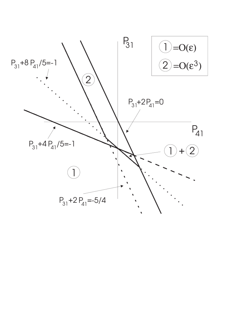
Figure 1: Stability regime for NLS ($d_{1}>0$)

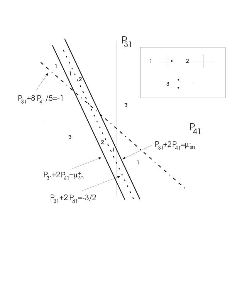
Figure 2: Stability regime for CGL ($d_{1}>0$)

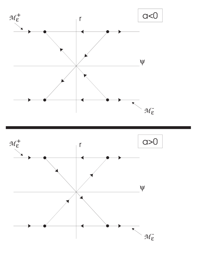
Figure 3: Projected flow onto $\{s=0\}\,(a=(d_{1}+d_{3}+2d_{4})(d_{1}+d_{3}+8d_{4}/5))$

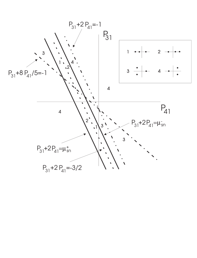
Figure 4: Zeros of $E(\gamma,\epsilon)\,(d_{1}>0)$

References

- [1] J. Alexander, R. Gardner, and C.K.R.T. Jones. A topological invariant arising in the stability of travelling waves. J. reine angew Math., 410:167–212, 1990.
- [2] P. Bollerman, A. van Harten, and G. Schneider. On the justification of the Ginzburg-Landau approximation. In Nonlinear dynamics and pattern formation in the natural environment, pages 20–36. Longman, Harlow, 1995.
- [3] A. Bose and C.K.R.T. Jones. Stability of the in-phase travelling wave solution in a pair of coupled nerve fibres. Indiana U. Math. J., 44(1):189–220, 1995.
- [4] S. Burtsev and R. Camassa. Nonadiabatic dynamics of dark solitons. J. Opt. Soc. Am. B, 14(7):1782–1787, 1997.
- [5] X.-J. Chen and Z.-D. Chen. Effects of nonlinear gain on dark solitons. IEEE J. Quantam Elect., 34(7):1308–1311, 1998.
- [6] X.-J. Chen, Z.-D. Chen, and N.-N. Huang. A direct perturbation theory for dark solitons based on a complete set of the squared Jost functions. J. Phys. A: Math. Gen., 31(33):6929–6947, 1998.
- [7] P. Collet and J.-P. Eckmann. The time-dependent amplitude equation for the Swift-Hohenberg problem. Comm. Math. Phys., 132:139–153, 1990.
- [8] A. Doelman. Slow time-periodic solutions of the Ginzburg-Landau equation. Phys. D, 40(2):156–172, 1989.
- [9] A. Doelman. Travelling waves in the complex Ginzburg-Landau equation. J. Nonlinear Science, 3:225–266, 1993.
- [10] A. Doelman. Breaking the hidden symmetry in the Ginzburg-Landau equation. Physica D, 97(4):398–428, 1996.
- [11] A. Doelman and W. Eckhaus. Periodic and quasi-periodic solutions of degenerate modulation equations. Physica D, 53:249–266, 1991.
- [12] A. Doelman, R. Gardner, and T. Kaper. Stability analysis of singular patterns in the 1-D Gray-Scott model II: rigorous theory. (in preparation).
- [13] J. Duan and P.Holmes. Fronts, domain walls, and pulses in a generalized Ginzburg-Landau equation. Proc. Edinburgh Math. Soc., 38:77–97, 1995.
- [14] W. Eckhaus. On modulation equations of the Ginzburg-Landau type. In ICIAM 91: Proc. 2nd Int. Conf. Ind. Appl. Math., pages 83–98, 1992.
- [15] N. Fenichel. Persistence and smoothness of invariant manifolds for flows. Indiana U. Math. J., 21:193–226, 1973.
- [16] R. Gardner. Stability and Hopf bifurcation of steady state solutions of a singularly perturbed reaction-diffusion system. SIAM J. Math. Anal., 23(1):99–149, 1992.
- [17] R. Gardner and C.K.R.T. Jones. Travelling waves of a perturbed diffusion equation arising in a phase field model. Indiana U. Math. J., 38(4):1197–1222, 1989.
- [18] R. Gardner and C.K.R.T. Jones. Stability of travelling wave solutions of diffusive predator-prey systems. Trans. AMS, 327(2):465–524, 1991.
- [19] R. Gardner and K. Zumbrun. The gap lemma and geometric criteria for instability of viscous shock profiles. Comm. Pure Appl. Math., 51(7):797–855, 1998.
- [20] A. Van Harten. On the validity of the Ginzburg-Landau equation. J. Nonlinear Sc., 1:397–422, 1991.
- [21] P. Holmes. Spatial structure of time-periodic solutions of the Ginzburg-Landau equation. Physica D, 23:84–90, 1986.
- [22] H. Ikeda, M. Matsumoto, and A. Hasegawa. Transmission control of dark solitons by means of nonlinear gain. Opt. Lett., 20(10):1113–1115, 1995.
- [23] H. Ikeda, M. Matsumoto, and A. Hasegawa. Stabilization of dark-soliton transmission by means of nonlinear gain. J. Opt. Soc. Am. B, 14(1):136–143, 1997.
- [24] C.K.R.T. Jones. Stability of the travelling wave solutions of the Fitzhugh-Nagumo system. Trans. AMS, 286(2):431–469, 1984.
- [25] C.K.R.T. Jones. Geometric singular perturbation theory. In R. Johnson, editor, Lecture Notes in Mathematics 1609. Springer-Verlag, New York, 1995.
- [26] C.K.R.T. Jones, T. Kapitula, and J. Powell. Nearly real fronts in a Ginzburg-Landau equation. Proc. Roy. Soc. Edin., 116A:193–206, 1990.
- [27] T. Kapitula. Stability of weak shocks in systems. Indiana U. Math. J., 40(4):1193–1219, 1991.
- [28] T. Kapitula. On the nonlinear stability of plane waves for the Ginzburg-Landau equation. Comm. Pure Appl. Math., 47(6):831–841, 1994.
- [29] T. Kapitula. Singular heteroclinic orbits for degenerate modulation equations. Physica D, 82(1&2):36–59, 1995.
- [30] T. Kapitula. Existence and stability of singular heteroclinic orbits for the Ginzburg-Landau equation. Nonlinearity, 9(3):669–686, 1996.
- [31] T. Kapitula. Bifurcating bright and dark solitary waves for the perturbed cubic-quintic nonlinear Schrödinger equation. Proc. Roy. Soc. Edinburgh, 128A:585–629, 1998.
- [32] T. Kapitula. The Evans function and generalized Melnikov integrals. SIAM J. Math. Anal., 30(2):273–297, 1999.
- [33] T. Kapitula and S. Maier-Paape. Spatial dynamics of time periodic solutions for the Ginzburg-Landau equation. Z. angew Math. Phys., 47(2):265–305, 1996.
- [34] T. Kapitula and B. Sandstede. A novel instability mechanism for bright solitary-wave solutions to the cubic-quintic Ginzburg-Landau equation. J. Opt. Soc. Am. B, 15:2757–2762, 1998.
- [35] T. Kapitula and B. Sandstede. Stability of bright solitary wave solutions to perturbed nonlinear Schrödinger equations. Physica D, 124(1–3):58–103, 1998.
- [36] J. Lega and S. Fuave. Traveling hole solutions to the complex Ginzburg-Landau equation as perturbations of nonlinear Schrödinger dark solitons. Physica D, 102:234–252, 1997.
- [37] Y. Li and K. Promislow. The mechanism of the polarizational mode instability in birefringent fiber optics. (preprint).
- [38] P. Marcq, H. Chatë, and R. Conte. Exact solutions of the one-dimensional quintic complex Ginzburg-Landau equation. Physica D, 73:305, 1994.
- [39] A. Markushevich. Theory of Functions. Chelsea Publishing Co., New York, 1985.
- [40] A. Mielke and G. Schneider. Attractors for modulation equations on unbounded domains - existence and comparison. Nonlinearity, 8(5):743–768, 1995.
- [41] S. Popp, O. Stiller, I. Aranson, and L. Kramer. Hole solutions in the 1d complex Ginzburg-Landau equation. Physica D, 84(3-4):398–423, 1995.
- [42] J. Rubin. Stability and bifurcations of standing pulse solutions to an inhomogeneous reaction-diffusion system. (to appear in Proc. Roy. Soc. Edinburgh A).
- [43] J. Rubin and C.K.R.T. Jones. Bifurcations and edge oscillations in the semiconductor Fabry-Pérot interferometer. Opt. Comm., 140:93–98, 1997.
- [44] W. Van Saarloos and P. Hohenberg. Fronts, pulses, sources, and sinks in the generalized complex Ginzburg-Landau equation. Physica D, 56D:303–367, 1992.
- [45] B. Sandstede. Stability of multiple-pulse solutions. Trans. Amer. Math. Soc., 350:429–472, 1998.
- [46] G. Schneider. Error estimates for the Ginzburg-Landau approximation. Z angew Math. Phys., 45:433–457, 1994.
- [47] G. Schneider. Global existence via Ginzburg-Landau formalism and pseudo-orbits of Ginzburg-Landau approximations. Comm. Math. Phys., 164:157–179, 1994.
- [48] R. Silverman. Introductory Complex Analysis. Dover Publications, Inc., New York, 1972.
- [49] O. Stiller, S. Popp, I. Aranson, and L. Kramer. All we know about hole solutions in the CGLE. Physica D, 87:361–370, 1995.
- [50] O. Stiller, S. Popp, and L. Kramer. From dark solitons in the defocusing nonlinear Schrödinger to holes in the complex Ginzburg-Landau equation. Physica D, 84(3-4):424–436, 1995.