[

Localized Structures in Nonlinear Lattices with Diffusive Coupling and External Driving

Abstract

We study the stabilization of localized structures by discreteness in one-dimensional lattices of diffusively coupled nonlinear sites. We find that in an external driving field these structures may lose their stability by either relaxing to a homogeneous state or nucleating a pair of oppositely moving fronts. The corresponding bifurcation diagram demonstrates a cusp singularity. The obtained analytic results are in good quantitative agreement with numerical simulations.

]

The problem of dynamics in discrete nonlinear lattices arises in diverse physical, biological, and engineering systems. Among the examples are interaction of charge- and spin-density waves with impurities in correlated electron materials [1, 2], arrays of Josephson junctions [2], calcium release waves in living cells [3], systems of coupled nonlinear oscillators [4], etc. Of special interest are lattices with continuous coupling between the nonlinear sites, because of their rich dynamical behavior. In Ref. [5] such systems have been shown to carry propagating burst waves. The role of localized structures as nucleation embryos in driven nonlinear systems is of wide importance [6], but the influence of lattice discreteness on nucleation and transport has received much less attention to date. We will show in this Letter that lattice discreteness indeed results in qualitatively new phenomena.

Below we study the stabilization of localized structures by discreteness in a system consisting of a lattice of diffusively coupled nonlinear sites. We investigate the properties of such structures and different mechanisms of their instabilities. We find a hysteresis effect in the nucleation of propagating fronts from the localized structures in an external field. We obtain our results analytically and confirm them by numerical simulations of the full system dynamics. Our system has relaxational dynamics given by $\partial u/\partial t=-\delta{\mathcal{E}}/\delta u\,$, where ${\mathcal{E}}$ is the system energy functional, $u$ is the order parameter, and $\delta/\delta u$ is a variational derivative. We consider the energy functional of the following form

$${\mathcal{E}}[u]\;=\;\frac{D}{2}\int\left(\frac{\partial u}{\partial x}\right)^{2}dx\;+\;\alpha\,\sum_{i}{\mathcal{F}}[u_{i}]\;.$$ (1)

Here $D$ is the diffusive coupling, ${\mathcal{F}}$ is the discrete nonlinear potential, $\alpha$ is the potential amplitude, and the sum is over all lattice sites $i\,$. We study the behavior of system (1) with bistable dynamics. The details of the potential shape are not important so long as it has at least two minima, $u=u_{-}$ and $u=u_{+}$ separated by a barrier with a maximum at $u=u_{0}\,$. The simplest example of such a potential ${\mathcal{F}}$ is a fourth degree polynomial ($\phi^{4}$). Here we study the sine-Gordon potential, because of its applicability to modeling the dynamics of charge density waves [1]. Although this potential has an infinite number of wells, for the localization problem studied in this Letter, only two neighboring minima are relevant. The potential has a form

$${\mathcal{F}}[u_{i}]\;=\;-\cos u_{i}-E\,u_{i}\;,$$ (2)

where $E$ is the applied external field. The field is required to make the depths of the potential wells different and thus allow for the propagation of fronts from less stable to more stable states. For potential (2), these stable states are $u_{-}=\arcsin E\,,\,u_{+}=u_{-}+2\pi\,,\,u_{0}=\pi-u_{-}\,$. The system dynamics are then governed by

$$u_{t}\;=\;\beta u_{xx}\;+\;\sum_{i}\delta(x-i)(-\sin u+E)\;,$$ (3)

with the space and time rescaled as $x\rightarrow x/d$ ($d$ is the distance between sites) and $t\rightarrow t\alpha\,$, respectively. The renormalized dimensionless diffusive coupling is $\beta=D/\alpha d^{2}\,$.

When $\beta\gg 1\,$, the system is in the continuous limit, where it is described by the overdamped sine-Gordon equation: $u_{t}=\beta u_{xx}-\sin u+E\,$. If one starts with the bulk of the system in the state $u=u_{-}\,$, below the barrier maximum $u_{0}\,$, and a finite size nucleus of the state $u=u_{+}\,$, above the maximum, then, for $E>0\,$, there exists a critical size of the nucleus. If the nucleus exceeds this critical size, it breaks into a pair of oppositely moving fronts; otherwise it relaxes back to the bulk state. We show that introducing discreteness into the system can stabilize the critical nucleus as localized structure.

In the discrete regime, $\beta\lesssim 1\,$, the system demonstrates substantially richer behavior. Well-separated fronts undergo a pinning-depinning transition from stationary kinks to propagating burst waves, which are periodic in a traveling-wave reference frame [5]. A stabilized nucleus represents a bound pair of kink and antikink. There exists a hierarchy of nuclei with differing numbers of sites at the state $u=u_{+}\,$, above the maximum. The distance between the kink and the antikink increases with the number of these sites, and the binding energy rapidly decays. Since the nucleation is caused by local fluctuations, the physically most important nuclei are those with small numbers of sites. As the parameters vary, a nucleus may lose its stability. Fig. 1 shows two alternative scenaria of one-site nucleus destabilization: (a) breaking to a pair of burst waves and (b) relaxation to the bulk state.

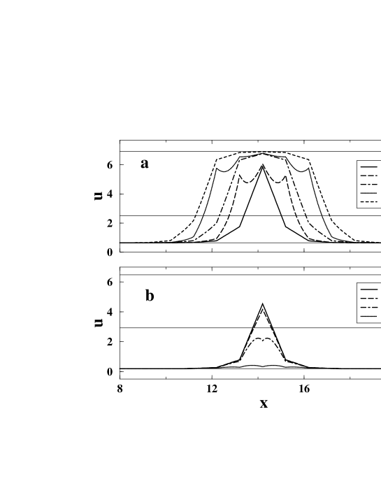
FIG. 1.: Successive profiles of the numerical solution $u(x)\,$ of Eq. (3), starting from a one-site nucleus. (a) Nucleation of two oppositely moving burst waves; $E=0.6\,,\,\beta=0.13\,$. (b) Relaxation to the bulk state $u=u_{-}\,$; $E=0.2\,,\,\beta=0.17\,$. For both cases the system length is $L=30\,$, the number of grid-points is $300\,$, time step $dt=2\times 10^{-5}\,$.

The bifurcation diagram of one- and two-site nuclei along with a single front in the ($E\,,\beta$) plane is shown in Fig. 2. The single kink is pinned below its bifurcation line and turns into a propagating burst wave above the line. Each nucleus is stable below its bifurcation line, which consists of two branches. Crossing the right or left branch upward results in the nucleation of a pair of burst waves or relaxation to the bulk state, $u=u_{-}\,$, respectively. The two branches intersect at a singular point, known as a cusp catastrophe [7]. We see in Fig. 2 that the nucleation of burst waves from localized nuclei demonstrates hysteresis, i.e. there is a parameter range, where a localized nucleus is stable, while a single front already propagates. The bifurcation lines for multi-site nuclei look similar. The field value at the singular point on each of the lines goes to $\infty\,$ and $\beta\to 0$, with the number of sites in the nucleus, due to the increasing separation of kinks. Note that the hysteresis and the nucleation phenomena mentioned above happen below the threshold driving strength ($|E|=1$ in Fig. 2), at which the effective potential from Eq. (2) loses its minima.

For any stationary solution, the dynamic equation (3) reduces to the following tridiagonal system of algebraic equations for $u_{i}$’s, the values of $u$ at the sites $x_{i}$’s,

$$\beta\,(u_{i+1}+u_{i-1}-2u_{i})-\sin u_{i}+E\;=\;0\;.$$ (4)

This arises because, in the stationary regime, Eq. (3) between the sites turns into a one-dimensional Laplace equation with linear solutions.

We notice that the maximum value of $\beta$ on the one-site nucleus bifurcation line in Figure 2, is $\sim 0.25\,$, i.e. deep in the discrete (small $\beta$) regime, which ends near $\beta\sim 1\,$. It is, therefore, natural to study the stability of the nucleus, taking $\beta$ as a small parameter of the analysis.

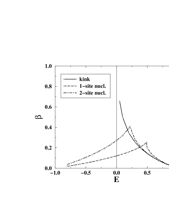
FIG. 2.: Numerically obtained bifurcation diagram of kink and one- and two-site nuclei. Parameters are as in Fig. 1.

The following three sites are the key elements of our analysis: the site of the nucleus, $i=n\,$, and its two nearest neighbors, $i=n\pm 1\,$, with the corresponding field values $u_{n}$ and $u_{n\pm 1}\,$. The symmetry of the nucleus implies that $u_{n+1}=u_{n-1}\equiv u^{*}\,$. The neighboring sites are both equivalent to the “front site” on a single kink. They are most active in a sense that they are the first candidates to cross the threshold value $u_{0}$, if the stationary solution becomes unstable. It can be shown (cf. results of Ref. [5] for a single kink) that the field value at the other sites decays with the distance from the front site down to $u_{-}\,$, as $u_{n\pm k}-u_{-}\sim\beta^{k-1}\,$ (for $k=2,3,\ldots$). Consider the stability analysis to first order in $\beta\,$. Then only the abovementioned three sites make a nontrivial contribution to the system stability properties, which leaves only two independent variables, $u_{n}$ and $u^{*}\,$. Using the corresponding two equations from the system (4), we reduce them to one equation for the “active” value $u^{*}$

$$g(u^{*})\; \equiv \;2\beta\,(u_{-}-u^{*})-2\sin u^{*}+3E$$ (5)

$$- \sin\left[2u^{*}-u_{-}+\frac{1}{\beta}(\sin u^{*}-E)\right]\;=\;0\;.$$ (6)

The solution of Eq. (6) is represented graphically in Fig. 3. The case of the right (breaking) branch of the one-site nucleus bifurcation line (see Fig. 2) corresponds to Fig. 3(a). Then below the bifurcation line, the function $g(u)$ in Eq. (6) is given by the solid line, and the equation has four solutions (open circles in the figure). To determine the stability of these solutions, one has to linearize system (4) and find the eigenvalues of the obtained linear problem. We note that the maximum eigenvalue $\lambda_{max}$ is responsible for the stability of the most active front site with $u=u^{*}\,$. This means that near the bifurcation line only $\lambda_{max}$ can change sign, whereas all other eigenvalues remain negative. To find $\lambda_{max}$, we linearize Eq. (6) and conclude that the 1st and the 3rd solutions for $u^{*}$ have $\lambda_{max}<0\,$, while the 2nd and the 4th solutions have $\lambda_{max}>0\,$. The two former solutions are, therefore, the stable nodes, and the two latter solutions are saddles with one unstable direction in the phase space.

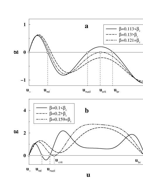
FIG. 3.: Solution of Eq. (6). (a) $E=0.6\,,\,\beta_{c}=0.121\,$; (b) $E=0.2\,,\,\beta_{c}=0.159\,$.

The 1st solution, however, is trivial in the sense that all sites are in the bulk state $u=u_{-}\,$. This leaves the single nontrivial stable solution, $u_{nucl}$ in Fig. 3. As $\beta$ increases, the stable solution and the right saddle, $u=u_{br}\,$, approach each other and eventually merge at $\beta=\beta_{c}\,$. This occurs when the maximum of curve $g(u)$ in Fig. 3(a) touches the line $g=0\,$, at $u=u_{crit}$. Apparently the two corresponding maximum eigenvalues both become zero, which implies a saddle-node bifurcation. Further increase of $\beta$ leaves the system without a stationary solution, and the nucleus breaks, leading to the formation of a pair of oppositely moving burst waves [Fig. 1(a)].

Stability analysis of the left (relaxation) branch of the bifurcation line (see Fig. 2) can be made analogously, using Fig. 3(b). The difference is that now the stable solution merges with the left (relaxation) saddle, $u=u_{rel}\,$, and the nucleus relaxes to the bulk state [Fig. 1(b)].

It appears that the first-order analysis is insufficient for the quantitative comparison of our theory with numerical simulations of Eq. (3). To improve our predictions, we have developed the stability analysis to second order in $\beta\,$. In this case one has to consider the nucleus and two of its neighbors from each side. Symmetry of the problem reduces the number of independent variables from five to three, and we deal with three corresponding equations from system (4). We then perform the same procedure as for the first-order stability analysis described above. In Fig. 4 we plot the resulting bifurcation line for the single-site nucleus along with the results of the simulations from Fig. 2. We see in Fig. 4 that our theoretical prediction is in good quantitative agreement with the simulations.

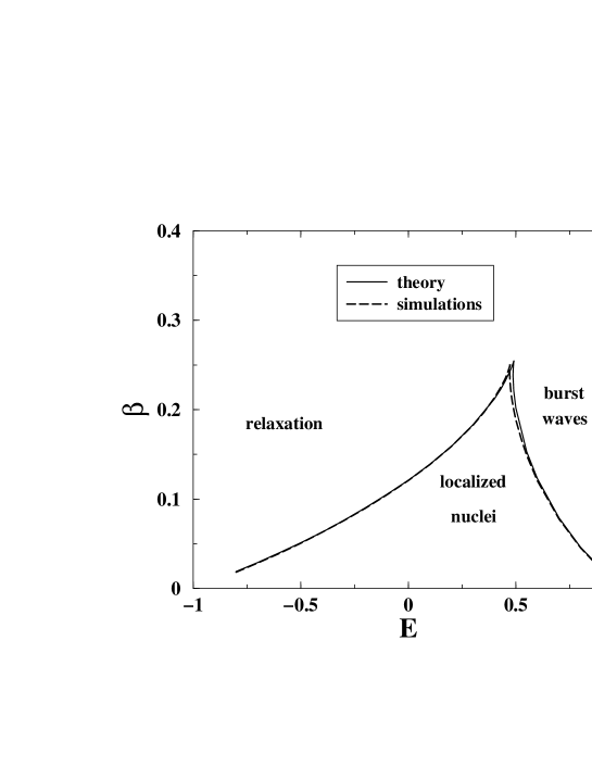
FIG. 4.: Comparison between analytical and numerical bifurcation lines for a one-site nucleus. Parameters as in Fig. 1.

We now describe the physical mechanisms of the obtained phenomena of relaxation and break-up of localized nuclei. In the parameter regime below the bifurcation line, the energy functional ${\mathcal{E}}$, Eq. (1), possesses a minimum in the functional space, which corresponds to a stable nucleus. Separatrices connect this minimum to the two neighboring unstable solutions (saddles). If one starts with an initial condition in either of these saddles slightly perturbed in the direction of the minimum, the system evolves along the separatrix until it relaxes at the minimum. If one parameterizes the position on the separatrix with an arclength $s$, defined as $ds^{2}=dt^{2}\int(\partial u/\partial t)^{2}dx\,$, the system dynamics take a simple gradient form, $ds/dt=-d{\mathcal{E}}(s)/ds\,$.

In Fig. 5 we plot the dependence of energy ${\mathcal{E}}$ on $s\,$ from numerical simulations. Fig. 5(a) shows ${\mathcal{E}}(s)$ near the break-up branch of the bifurcation line. We see in the figure that, for the stable nucleus (solid line), the energy indeed has a minimum and two neighboring maxima, corresponding to the saddles of the dynamics. When the nucleus loses stability (dashed line), the minimum merges with the right (break-up) saddle. Then the nucleus turns into a pair of burst waves and the energy begins monotonically decreasing. If we start with an initial condition slightly to the right of the break-up saddle then the system develops a pair of burst waves, even in the stable nucleus regime. This is the manifestation of the nucleation hysteresis effect, since the bound nucleus is still stable in the parameter range for which a well-separated front already bursts and propagates. If, on the other hand, we start to the left of the relaxation saddle, then the system will relax to the homogeneous bulk state $u=u_{-}$ for both stable and unstable nuclei.

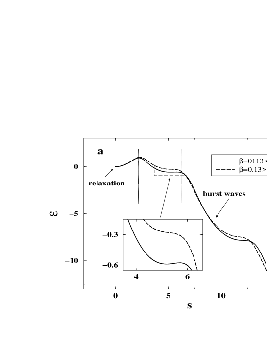
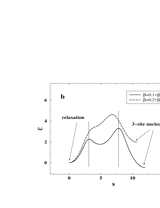
FIG. 5.: Energy ${\mathcal{E}}$ vs arclength $s$ near (a) break-up branch ($E=0.6$) and (b) relaxation branch ($E=0.2$) of the bifurcation line of a one-site nucleus.

The system behavior near the relaxation branch of the bifurcation line is different, see Fig. 5(b). As $\beta$ crosses the critical value, the minimum of the functional merges with the left (relaxation) saddle, and the system relaxes to the homogeneous bulk state. The same thing happens if we start to the left of this saddle, for the regime of parameters where the nucleus is stable. However, if we start slightly to the right of the break-up saddle, then the nucleus at first starts breaking, but then relaxes to the three-site nucleus, rather than developing into the pair of separated burst waves.

In conclusion, we have demonstrated that nonlinear lattices with diffusive coupling possess localized structures, in certain parameter regimes. We have shown that these structures can be destroyed in two alternative scenaria: (i) break-up into a pair of oppositely propagating burst waves, and (ii) relaxation to a homogeneous state. We have found hysteresis in the burst-wave nucleation from a localized embryo, appearing as the difference between the stability thresholds of nucleus break-up and burst-wave propagation. We have given a theoretical description of these phenomena in terms of the energy functional of our system. The predictions of our theory are in a good quantitative agreement with numerical simulations of the full system. Our interesting directions for future research: the influence of the localized structures on thermal nucleation [6], dynamics of localized structures in corresponding two- and three-dimensional systems, experimental studies of stable and unstable nuclei in materials, etc. We note that, though we have studied lattices with continuous coupling, the stability analysis has been performed for stationary localized structures from Eq. (4). Therefore, the obtained stability properties of these structures should remain intact for completely discrete systems, such as arrays of Josephson junctions [2] or lattices of nonlinear oscillators [4].

We appreciate fruitful discussions with D. K. Campbell and J. E. Pearson. This research is supported by the Department of Energy under contract W-7405-ENG-36.

REFERENCES

- [1] H. Fukuyama and P. A. Lee, Phys. Rev. B17, 535 (1978); S. N. Coppersmith, Phys. Rev. Lett.65, 1044 (1990); A. R. Bishop, B. Horovitz, and P. S. Lomdahl, Phys. Rev. B38, 4853 (1988); G. Gruner, Rev. Mod. Phys. 60, 1129 (1988); ibid 66, 1 (1994).
- [2] L. M. Floria and J. J. Mazo, Adv. Phys. 45, 505 (1996).
- [3] A. E. Bugrim, A. M. Zhabotinsky, and I. R. Epstein, Biophys. J. 73, 2897 (1997); J. Keizer, G. D. Smith, S. Ponce Dawson, and J. E. Pearson, Biophys. J. 75, 595 (1998).
- [4] M. Locher, D. Cigna, and E. R. Hunt, Phys. Rev. Lett.80, 5212 (1998); J. F. Lindner, S. Chandramouli, A. R. Bulsara, M. Locher, and W. L. Ditto, Phys. Rev. Lett.81, 5048 (1998).
- [5] I. Mitkov, K. Kladko, and J. Pearson, Phys. Rev. Lett.81, 5453 (1998).
- [6] M. Buttiker, R. Landauer, Phys. Rev. Lett.43, 1453 (1979); F. Marchesoni, L. Gammaitoni, and A. R. Bulsara, Phys. Rev. Lett.76, 2609 (1996).
- [7] V. I. Arnol’d (Ed.), Dynamical Systems V, Bifurcation Theory (Springer-Verlag, 1994).