Instabilities and Spatio-Temporal Chaos in Hexagon Patterns with Rotation

Abstract

The dynamics of hexagon patterns in rotating systems are investigated within the framework of modified Swift-Hohenberg equations that can be considered as simple models for rotating convection with broken up-down symmetry, e.g. non-Boussinesq Rayleigh-Bénard or Marangoni convection. In the weakly nonlinear regime a linear stability analysis of the hexagons reveals long- and short-wave instabilities, which can be steady or oscillatory. The oscillatory short-wave instabilities can lead to stable hexagon patterns that are periodically modulated in space and time, or to a state of spatio-temporal chaos with a Fourier spectrum that precesses on average in time. The chaotic state can exhibit bistability with the steady hexagon pattern. There exist regimes in which the steady hexagon patterns are unstable at all wavenumbers.

PACS: 47.54.+r, 47.27.Te, 47.20.Dr, 47.20.Ky

Keywords: Hexagon Patterns, Rotating Convection, Swift-Hohenberg Equation, Sideband Instabilities, Spatio-temporal Chaos

I Introduction

Patterns arising from hydrodynamic instabilities have become a paradigm for the investigation of dynamical systems with many degrees of freedom. In particular Rayleigh-Bénard convection has been studied experimentally and theoretically in great detail. In recent years the focus of investigation has turned to patterns that are spatially and possibly also temporally complex. Various types of such states of spatio-temporal chaos have been identified. Great interest has, for example, found the spiral-defect chaos that is observed in convection of fluids with not too large Prandtl number [2, 3]. It is characterized by the appearance and disappearance of spirals in the convection patterns that are separated by domains of straight or slightly curved convection rolls. Spiral-defect chaos has not been found directly at onset of convection. Thus, it is not accessible by weakly nonlinear theory. From a theoretical point of view another type of spatio-temporal chaos has therefore been very attractive since it arises directly at onset. It is observed in rotating convection and is due to the Küppers-Lortz instability through which all straight-roll states become unstable to rolls of a different orientation if the rotation rate is sufficiently large [4]. In a simple three-mode model for rolls rotated by $120^{o}$ with respect to each other this instability leads to a structurally stable heteroclinic orbit connecting the three sets of rolls [5, 6]. In large aspect-ratio experiments [7, 8, 9] and numerical simulations of Ginzburg-Landau equations [10] and of order-parameter models [11, 12] the switching between the different orientations looses coherence across the system and domains of almost straight rolls of different orientations form that persistently invade each other in an irregular manner.

The character of a spatio-temporally chaotic state is expected to depend strongly on the planform of the underlying pattern. Thus, spatio-temporal chaos arising from instabilities of stripes (or rolls) will differ from that of square or hexagonal patterns. For instance, in hexagon (or square) patterns the bending of rolls that is widely observed in Rayleigh-Bénard convection is strongly suppressed. Instead, the appearance of disorder in a hexagonal pattern might resemble more the melting of a ‘crystal’. There have been only a few studies of transitions to spatio-temporal chaos from square or hexagon patterns. Experimental investigations have been made on parametrically driven surface waves [13, 14] and on a chemical system [15].

In the present work we consider hexagon patterns in systems with broken up-down symmetry and study the effect of a breaking of the chiral symmetry on their stability and dynamics. It is motivated by the complex dynamics ensuing from the Küppers-Lortz instability of convection rolls, where the chiral symmetry is broken by a global rotation of the system. From a general weakly nonlinear analysis of the three modes making up the hexagon patterns it is known that a breaking of the up-down symmetry transforms the structurally stable heteroclinic cycle that results from the Küppers-Lortz instability within the three-mode model into a periodic orbit of oscillating hexagons [1, 16, 17]. This periodic orbit arises from a Hopf bifurcation, which replaces the steady instability of the hexagonal pattern that leads to rolls [1, 16].

We are interested in the question which additional instabilities can arise if one goes beyond the three-mode model and allows arbitrary perturbation modes. Of particular interest are situations in which such perturbations lead to persistent dynamics. One possible approach is to extend the three-mode amplitude equations to three coupled Ginzburg-Landau equations that also allow for a slow spatial variation of the amplitudes [35]. The slowness of the space dependence implies, however, that all perturbations to the hexagons are restricted to wavevectors close to those of the hexagon modes. In particular, only modes making a small angle with respect to the hexagon modes can be treated. Furthermore, the Ginzburg-Landau equations cannot be expected to be suitable for general numerical simulations of unstable hexagon patterns in large systems since the choice of the three carrier modes making up the hexagons strongly breaks the isotropy of the system. Only in the unlikely case that the perturbation wavevectors remain close to the wavevectors of the hexagon modes for all times would the Ginzburg-Landau equations be adequate.

The goal of our investigation is to explore what type of instabilities can appear due to the breaking of the chiral symmetry and whether they can lead to persistent regular or irregular dynamics. It is therefore important to allow arbitrary perturbation modes and to preserve the isotropy of the system. Thus, we investigate a simple model of the Swift-Hohenberg type [18, 19, 20]. Such models have been widely used to address general questions regarding the dynamics of patterns (e.g. [17, 19, 12, 21, 22, 23]). If the patterns arise from a long-wave instability equations of the Swift-Hohenberg type can be derived systematically in a long-wave analysis. This has been done, for instance, for buoyancy-driven convection with asymmetric boundary conditions [24] and for Marangoni convection [25, 32]. In both cases the onset of convection occurs at long wavelengths if the boundaries are poor conductors. If the wavenumber at onset is finite the Swift-Hohenberg cannot be derived rigorously from the basic equations (e.g. Navier-Stokes equations), but they can be obtained as approximate order-parameter models by expanding the nonlinear interaction terms (e.g. [19, 20]).

We perform a general linear stability analysis of the weakly nonlinear hexagon pattern and pay particular attention to destabilizing modes that are rotated with respect to the hexagon pattern. In the absence of rotation such general stability analyses of hexagonal patterns have been performed for the full fluid equations for Marangoni convection [26] as well as within coupled Ginzburg-Landau equations [27]. Some results are also available for weakly nonlinear Marangoni convection in the presence of rotation [28]. We complement the stability analysis with direct simulations of the order-parameter equation to investigate the nonlinear behavior resulting from the instabilities. We find that the hexagonal pattern can become unstable at all wavelengths, resulting in spatio-temporally chaotic states. Moreover, even for parameters for which stable hexagon patterns exist, persistent periodic and irregular dynamics are found, implying bistability of ordered and disordered states.

The paper is organized as follows. In Section II we introduce two order-parameter models and set up the linear stability analysis of the weakly nonlinear hexagons. In Section III the results of that analysis are presented. We discuss the different types of instabilities and the resulting stability regions of hexagonal patterns. In Section IV numerical simulations of the order-parameter equation are used to confirm the stability analysis and to investigate the nonlinear evolution ensuing from it. Conclusions are found in Section V.

II The Model and Linear Stability Analysis

Spatially periodic hexagon patterns with small amplitude arising from a weakly transcritical bifurcation can be described systematically by coupled equations for the complex amplitudes $A$, $B$, and $C$ of the three stripe (roll) components

$$\frac{\partial A}{\partial\tau_{2}}=R_{2}A+2\,\zeta B^{*}C^{*}+\left(f_{1}{|A|}^{2}+f_{2}{|B|}^{2}+f_{3}{|C|}^{2}\right)A,$$ (1)

where $\tau_{2}$ is a slow time, $R_{2}$ a reduced control parameter and the difference between the cubic coupling coefficients $f_{2}$ and $f_{3}$ is proportional to the breaking of the chiral symmetry. The equations for $B$ and $C$ follow by cyclic permutation. To investigate the stability of these hexagons with respect to spatially varying perturbations the amplitudes could be allowed to be space-dependent which would lead to the inclusion of spatial derivatives in (1). The amplitude description breaks, however, the isotropy of the system and requires that the space dependence of the amplitudes be slow. This implies that only perturbations with wavevectors close to those making up the hexagon can be considered. In this study we are interested in particular in perturbations that are rotated with respect to the hexagons by an arbitrary amount and in dynamical, disordered states that may exhibit an essentially isotropic wavevector spectrum. Therefore the isotropy of the system needs to be preserved and Ginzburg-Landau-type amplitude equations are not sufficient to investigate the questions we are interested in.

For a first exploration of the impact of a chiral symmetry breaking on side-band perturbations of hexagons and their nonlinear evolution it is appropriate to preserve the isotropy of the system by considering a simple model equation rather than the full hydrodynamical problem. Detailed investigations of specific physical systems can then be performed as a second step guided by the results of the model equations.

In a number of studies Swift-Hohenberg-type models have provided valuable insight into the dynamics of patterns (e.g. [17, 19, 12, 21, 22, 23]). We consider here a minimal model of that type for an order parameter $\psi(x,y,t)$. In order to obtain stable hexagons in the absence of rotation we introduce a quadratic term $\alpha\psi^{2}$ that breaks the up-down symmetry $\psi\rightarrow-\psi$. The cubic scalar term $\psi^{3}$ of the original Swift-Hohenberg equation provides nonlinear saturation. To break the chiral symmetry nonlinear gradient terms have to be introduced. At leading order in the amplitude and the gradients this introduces an additional quadratic term and we are led to consider the model

$$\partial_{t}\psi = R\psi-(\nabla^{2}+1)^{2}\psi-\psi^{3}+\alpha\psi^{2}+\gamma\;\hat{e}_{z}\cdot(\nabla\psi\times\nabla(\nabla^{2}\psi)),$$ (2)

where $\hat{e}_{z}$ is the unit vector perpendicular to the $(x,y)$-plane. In these equations the bifurcation parameter is $R$ and the wavenumber of the bifurcating mode has been scaled to 1. The strength of the chiral symmetry-breaking is measured by $\gamma$.

It should be noted that the quadratic gradient term in (2) has the somewhat non-generic feature that it generates harmonics only from the interaction of modes with wavevectors of different magnitude. As a consequence, in the small-amplitude regime (1), for which $\alpha$ has to be assumed to be small, it does not modify the cubic coefficients $f_{i}$ in (1) and has therefore to this order no effect on strictly periodic hexagon patterns. In particular, the instability of hexagons that occurs with increasing $R$ is not oscillatory and does not lead to the periodic orbit of oscillating hexagons identified in [1, 16] (cf. Fig.3). Instead, the instability remains steady and leads directly to the roll solution as is the case in the absence of rotation. In this paper we focus on the stability of the steady hexagons with respect to side-band perturbations below that instability. Thus, the existence of the secondary branch of oscillating hexagons is not of central importance. We present most results for the minimal model (2).

The non-genericity of the quadratic gradient term in (2) can be addressed by introducing additional terms. One possibility is to introduce a quadratic term, e.g. $\beta(\nabla\psi)^{2}$, that allows $\alpha$ to be of $O(1)$ as long as $\alpha$ and $\beta$ together lead to $\zeta\ll 1$ in (1). Alternatively, a cubic term that breaks the chiral symmetry can be introduced, e.g. $g_{2}\;\hat{e}_{z}\cdot(\nabla\times(\nabla\psi)^{2}\nabla\psi)$. We thus have the extended model

$$\partial_{t}\psi = R\psi-(\nabla^{2}+1)^{2}\psi-\psi^{3}+\alpha\psi^{2}+\beta(\nabla\psi)^{2}+\gamma\;\hat{e}_{z}\cdot(\nabla\psi\times\nabla(\nabla^{2}\psi))+g_{2}\hat{e}_{z}\cdot(\nabla\times(\nabla\psi)^{2}\nabla\psi),$$ (3)

whose results we discuss briefly.

While we are using (2) and (3) as simple model equations, equations of that type can be obtained from the basic physical equation (e.g. the fluid equations) by expanding the interaction term in Fourier space [19, 30, 31]. In general, one then obtains additional nonlinear gradient terms. Similar equations can be derived systematically as long-wave equations (e.g. for buoyancy-driven convection with asymmetric boundary conditions [24] or for surface-tension driven convection without [25] and with rotation [32]).

We perform a weakly nonlinear analysis of (2) and (3), and start with a small amplitude expansion of $\psi$ on a hexagonal lattice,

$$\psi = \hskip 14.45377pt\epsilon\left\{Ae^{ikx}+Be^{ik(-x/2+y\sqrt{3}/2)}+Ce^{ik(-x/2-y\sqrt{3}/2)}\right\}$$ (7)

$$\mbox{}+\epsilon^{2}\left\{D_{000}+D_{200}e^{i2kx}+D_{020}e^{ik(-x+\sqrt{3}y)}+D_{002}e^{ik(-x-\sqrt{3}y)}\right.$$

$$\mbox{}\hskip 14.45377pt+\left.D_{1\overline{1}0}e^{ik(3x/2-y\sqrt{3}/2)}+D_{10\overline{1}}e^{ik(3x/2+y\sqrt{3}/2)}+D_{01\overline{1}}e^{ik\sqrt{3}y}\right\}$$

$$\mbox{}+c.c.+h.o.t.,$$

where $\epsilon\ll 1$ and $k$ is the wavenumber of the pattern. The Fourier amplitudes are functions of the slow time $\tau_{2}=\epsilon^{2}t$. The subscripts on the harmonics $D_{lmn}$ indicate how the Fourier mode is expressed in terms of the $O(\epsilon)$ modes; the first, second, and third subscripts indicate how many times $e^{ikx}$, $e^{ik(-x/2+y\sqrt{3}/2)}$, and $e^{ik(-x/2-y\sqrt{3}/2)}$ are factors of the Fourier mode, respectively. Bars over the subscripts indicate complex conjugates. For example, $D_{10\overline{1}}e^{ik(3x/2+y\sqrt{3}/2)}$ contains one $e^{ikx}$-mode and one complex conjugate of the $e^{ik(-x/2-y\sqrt{3}/2)}$-mode.

Inserting the expansion (7) into the model equations (2) and (3) and eliminating the terms involving $D_{lmn}$ at $O(\epsilon^{2})$,in each case one obtains at $O(\epsilon^{3})$ a set of amplitude equations of the form (1) for the amplitudes $A$, $B$, and $C$. In the case of the minimal model (2), the coefficients of (1) have the values

$$f_{1}=3,\qquad f_{2}=6,\qquad f_{3}=6,$$ (8)

and $R_{2}=(R-(k^{2}-1)^{2})/\epsilon^{2}$. Note that $R$ is expanded about the neutral curve for the specified hexagon wavenumber $k$, and not about $R=0$. To obtain a homogeneous scaling, we have assumed the bifurcation to be weakly transcritical, and hence

$$\zeta=\alpha/\epsilon\equiv O(1).$$ (9)

Note that the quadratic rotation term $\gamma\hat{e}_{k}\cdot(\nabla\psi\times\nabla(\nabla^{2}\psi))$ does not enter the amplitude equations (1) if $\alpha\ll 1$. In terms of the original variables, the amplitude for the steady hexagon solution is to this order given by

$$A=B=C={\frac{-\alpha-\sqrt{\alpha^{2}-(R-(k^{2}-1)^{2})\,(f_{1}+f_{2}+f_{3})}}{(f_{1}+f_{2}+f_{3})}}.$$ (10)

In the case of the extended model (3), the coefficients of (1) have the values

$$\zeta = \left\{\alpha+\frac{\beta k^{2}}{2}\right\}/\epsilon\equiv O(1),$$ (11)

$$f_{1} = 3-\left\{\frac{9}{2(6k^{2}-15k^{4})}+\frac{1}{k^{4}-2k^{2}}\right\}\beta^{2}k^{4},$$ (12)

$$f_{2,3} = 6\mp g_{2}k^{4}\sqrt{3}\mp\frac{2k^{6}\sqrt{3}}{4k^{2}-8k^{4}}\gamma\beta-\left\{\frac{4}{4k^{2}-8k^{4}}+\frac{1}{k^{4}-2k^{2}}\right\}\beta^{2}k^{4},$$ (13)

The effect of rotation is contained solely in $f_{2}$ and $f_{3}$ such that $f_{2}(\gamma,g_{2})=f_{3}(-\gamma,-g_{2})$. Note that in (12,13) $\alpha$ has been replaced by $\beta$ using (11). The hexagon solution is to this order given by

$$A=B=C={\frac{-(\alpha+{\frac{\beta k^{2}}{2}})-\sqrt{(\alpha+{\frac{\beta k^{2}}{2}})^{2}-(R-(k^{2}-1)^{2})\,(f_{1}+f_{2}+f_{3})}}{(f_{1}+f_{2}+f_{3})}}.$$ (14)

In either case, to study the stability of the hexagon solution $H(x,y)$ a general Floquet ansatz with modulation wavevector $(\tilde{q},\tilde{p})$ is made,

$$\psi=H(x,y)+\delta e^{i\tilde{q}x+i\tilde{p}y}P(x,y,t),$$ (15)

where $P(x,y)$ has the periodicity of the hexagonal lattice and $\delta\ll 1$. Being interested in the weakly nonlinear regime, we expand $H(x,y)$ and $P(x,y)$ in $\epsilon$ and obtain

$$\psi = \epsilon\left\{Ae^{ikx}+Be^{ik(-x/2+y\sqrt{3}/2)}+Ce^{ik(-x/2-y\sqrt{3}/2)}\right\}$$ (22)

$$\mbox{}+\epsilon\delta\left\{P_{000}e^{i(qx+py)}\right\}$$

$$\mbox{}+\epsilon^{2}\left\{D_{000}+D_{200}e^{i2kx}+D_{020}e^{ik(-x+\sqrt{3}y)}+D_{002}e^{ik(-x-\sqrt{3}y)}\right.$$

$$\mbox{}\hskip 14.45377pt\left.+D_{1\overline{1}0}e^{ik(3x/2-y\sqrt{3}/2)}+D_{10\overline{1}}e^{ik(3x/2+y\sqrt{3}/2)}+D_{01\overline{1}}e^{ik\sqrt{3}y}\right\}$$

$$\mbox{}+\epsilon^{2}\delta\left\{H_{0\overline{1}0}e^{i((q+k/2)x+(p-k\sqrt{3}/2)y)}+H_{100}e^{i((q+k)x+py)}+H_{00\overline{1}}e^{i((q+k/2)x+(p+k\sqrt{3}/2)y)}\right.$$

$$\mbox{}\hskip 14.45377pt\left.+H_{\overline{1}00}e^{i((q-k)x+py)}+P_{010}e^{i((q-k/2)x+(p+k\sqrt{3}/2)y)}+P_{001}e^{i((q-k/2)x+(p-k\sqrt{3}/2)y)}\right\}$$

$$\mbox{}+c.c.+h.o.t.$$

with the amplitudes of the perturbation modes depending on time. Here the notation for the $O(\epsilon)$ and $O(\epsilon^{2})$ modes is as before. The subscripts on the $O(\epsilon^{2}\delta)$ amplitudes indicate how many times the $e^{i(qx+py)}$-mode was multiplied by the indicated Fourier components that make up the original hexagon solution to create the harmonic mode. The reason for labelling some of the $O(\epsilon^{2}\delta)$ modes as $H$ and some as $P$ will become apparent below. In the expansion (22) we have combined the modulation wavevector $(\tilde{q},\tilde{p})$ with the basic wavevector $(k,0)$ of the hexagon pattern into the perturbation wavevector $(q=k+\tilde{q},p=\tilde{p})$. Thus, long-wave perturbations are characterized by $(q,p)$ being close to $(k,0)$.

As long as the wavevector $(q,p)$ of the perturbation mode $P_{000}$ is not close to the wavevector of one of the hexagon modes the harmonics $H_{lmn}$ and $P_{lmn}$ of $P_{000}$ are bounded away from the critical circle (cf. Fig.2 below). Thus, their damping is $O(1)$ and they can be eliminated in favor of $P_{000}$ and the hexagon modes $A$, $B$, and $C$. Consequently, they are small (of $O(\delta\epsilon^{2})$) compared to $P_{000}$. This results in an evolution equation for $P_{000}$ alone.

It turns out that the expansion (22) yields unsatisfactory results for the growth rate of the perturbation as a function of $\theta$. This is due to singularities that arise for $\theta=0$ and $\theta=\pm 60^{\circ}$. For $k=\sqrt{q^{2}+p^{2}}=1$, as $\theta\rightarrow 0$ the perturbation modes $P_{010}$ and $P_{001}$ approach the critical circle and their linear damping goes to zero. Thus, they cannot be eliminated adiabatically any more as signified by singularities in the growth rate for $P_{000}$. Similarly, when $\theta\rightarrow 60^{\circ}$ the mode $H_{0\bar{1}0}$ approaches the critical circle. The influence of the singularities at $0^{\circ}$ and $60^{\circ}$ on the eigenvalues is so large that they become unreliable over the whole range $0^{\circ}<\theta<60^{\circ}$.

FIG. 1.: Fourier space diagram showing the critical unit circle and location of the modes used in the final expansion of $\psi$ (cf. (32)). Indicated with arrows is an example of the combination of an $O(\epsilon\delta)$ perturbation mode and an $O(\epsilon)$ original hexagon mode driving a $O(\epsilon^{2}\delta)$ higher harmonic mode.

FIG. 2.: Fourier space diagram where $\theta\rightarrow 60^{\circ}$. Here the modes $H_{0\overline{1}0}$, $H_{0\overline{1}1}$, $H_{002}$, and $H_{\overline{1}00}$ approach the critical unit circle despite being of $O(\epsilon^{2}\delta)$, and thus drive a singularity when solved for.

In order to avoid the singularities, $P_{010}$ and $P_{001}$ are allowed to be of $O(\epsilon\delta)$, i.e. of the same order as the original perturbation mode $P_{000}$. Then at $O(\epsilon^{2}\delta)$ they drive the modes $P\,_{\overline{1}01}$ and $P\,_{\overline{1}10}$ leading to singularities in these modes for $\theta\rightarrow 0$. Hence, modes $P_{\overline{1}01}$ and $P\,_{\overline{1}10}$ must also be allowed to be of $O(\epsilon\delta)$. In fact, all modes that come close to the critical circle as $e^{i(qx+py)}$ approaches $e^{ix}$ must be kept at $O(\epsilon\delta)$. They are labelled $P_{lmn}$. This finally leads to the following expansion for $\psi$ (cf. Fig. 2),

$$\psi = \hskip 14.45377pt\epsilon\left\{Ae^{ikx}+Be^{ik(-x/2+y\sqrt{3}/2)}+Ce^{ik(-x/2-y\sqrt{3}/2)}\right\}$$ (32)

$$\mbox{}+\epsilon\delta\left\{P_{000}e^{i(qx+py)}+P_{010}e^{i((q-k/2)x+(p+k\sqrt{3}/2)y)}+P_{001}e^{i((q-k/2)x+(p-k\sqrt{3}/2)y)}\right.$$

$$\mbox{}\hskip 18.06749pt+\left.P_{\overline{1}10}e^{i((q-3k/2)x+(p+k\sqrt{3}/2)y)}+P_{\overline{1}01}e^{i((q-3k/2)x+(p-k\sqrt{3}/2)y)}+P_{\overline{2}00}e^{i((q-2k)x+py)}\right\}$$

$$\mbox{}+\epsilon^{2}\left\{D_{000}+D_{200}e^{i2kx}+D_{020}e^{ik(-x+\sqrt{3}y)}+D_{002}e^{ik(-x-\sqrt{3}y)}\right.$$

$$\mbox{}\hskip 14.45377pt\left.+D_{1\overline{1}0}e^{ik(3x/2-y\sqrt{3}/2)}+D_{10\overline{1}}e^{ik(3x/2+y\sqrt{3}/2)}+D_{01\overline{1}}e^{ik\sqrt{3}y}\right\}$$

$$\mbox{}+\epsilon^{2}\delta\left\{H_{\overline{1}00}e^{i((q-k)x+py)}+H_{100}e^{i((q+k)x+py)}+H_{00\overline{1}}e^{i((q+k/2)x+(p+k\sqrt{3}/2)y)}\right.$$

$$\mbox{}\hskip 14.45377pt+H_{0\overline{1}1}e^{i(qx+(p-k\sqrt{3})y)}+H_{002}e^{i((q-k)x+(p-k\sqrt{3})y)}+H_{\overline{1}02}e^{i((q-2k)x+(p-k\sqrt{3})y)}$$

$$\mbox{}\hskip 14.45377pt+H_{\overline{2}01}e^{i((q-5k/2)x+(p-k\sqrt{3}/2)y)}+H_{\overline{3}00}e^{i((q-3k)x+py)}+H_{\overline{2}10}e^{i((q-5k/2)x+(p+k\sqrt{3}/2)y)}$$

$$\mbox{}\hskip 14.45377pt+H_{\overline{1}20}e^{i((q-2k)x+(p+k\sqrt{3})y)}+H_{020}e^{i((q-k)x+(p+k\sqrt{3})y)}+H_{01\overline{1}}e^{i(qx+(p+k\sqrt{3})y)}$$

$$\mbox{}\hskip 14.45377pt+\left.H_{0\overline{1}0}e^{i((q+k/2)x+(p-k\sqrt{3}/2)y)}\right\}+c.c.+h.o.t.$$

Certain values of $(q,p)$ drive a resonance that is still not accounted for in the scaling of the modes. For $k=1$, as $\theta$ approaches $60^{\circ}$ the expansion breaks down again because the modes corresponding to $H_{0\overline{1}0},H_{0\overline{1}1},H_{\overline{1}00}$, and $H_{002}$ are now near the critical circle (cf. Fig. 2), but are still kept at $O(\epsilon^{2}\delta)$ in the expansion (32). Similarly, the expansion breaks down as $\theta$ approaches $-60^{\circ}$. Due to the $60^{\circ}$-periodicity of the expansion, we may restrict ourselves to $\theta$ between $-30^{\circ}$ and $30^{\circ}$, and thus avoid having to do an altered calculation for these situations. If $k=0.888$, a resonance occurs already for $\theta=\pm 30^{\circ}$. Since $k=.888$ is smaller than any hexagon wavenumber we consider, restricting $\theta$ to the range $-30^{\circ}$ to $30^{\circ}$ is adequate.

To summarize, in the expansion (32) all modes are retained that are excited at $O(\epsilon^{2})$ or $O(\epsilon^{2}\delta)$ by the perturbation modes or the hexagon modes. This is sufficient to determine the growth rates of the perturbation modes at $O(\epsilon^{3}\delta)$. The expansion remains well ordered as long as the hexagon wavenumber and the perturbation wavenumber are close to 1 and the angle $\theta$ is between $-30^{\circ}$ and $+30^{\circ}$.

We now substitute (32) into (2), expand, and use equation (10) to find the perturbation growth rates for the minimal model. For the extended model (3) and (14) are used. To obtain a unified description for the whole range of angles we reconstitute the perturbation equations at $O(\epsilon^{2}\delta)$ and $O(\epsilon^{3}\delta)$ by substituting in for all scaled amplitudes, e.g. $A={\cal A}/\epsilon$, $P_{lmn}={\cal P}_{lmn}/\epsilon\delta$, etc., as well as the scaled variables, $\zeta=\alpha/\epsilon$ or $\zeta=(\alpha+\beta/2)/\epsilon$ (depending on the model) and $R_{2}=(R-(k^{2}-1)^{2})/\epsilon^{2}$, and the scaled times, $\partial_{T}=\partial_{t}+\epsilon\partial_{\tau_{1}}+\epsilon^{2}\partial_{\tau_{2}}$. This leads to

$$\partial_{T}{\cal P}_{000} = (R-(q^{2}+p^{2}-1)^{2}){\cal P}_{000}$$ (34)

$$\mbox{}+{\cal B}^{*}{\cal P}_{010}f_{010}(q,p,k)+{\cal C}^{*}{\cal P}_{001}f_{001}(q,p,k)+\sum_{lmn}g_{lmn}(q,p,k)|{\cal A}|^{2}{\cal P}_{lmn},$$

where the sum goes over all six perturbation modes ${\cal P}_{lmn}$. The equations for the other amplitudes ${\cal P}_{lmn}$ follow by cyclic permutation within the circle of modes ($P_{000}$, $P_{010}$, $P_{\bar{1}10}$, $P_{\bar{2}00}$, $P_{\bar{1}01}$, $P_{001}$). It turns out that despite the assumption of weak transcriticality, (9) or (11), the coefficients of the quadratic terms involving ${\cal B^{*}}$ and ${\cal C^{*}}$ are not small in general. While the coefficients go to zero for $\theta\rightarrow 0$ and $\zeta=0$, they are of $O(1)$ for finite angles $\theta$. For finite angles and $k$ close to $1$, however, the modes ${\cal P}_{010}$ and ${\cal P}_{001}$ to which ${\cal P}_{000}$ is coupled are small rendering the quadratic terms again of the same order as the cubic terms.

III Linear Stability Results

The general stability analysis (34) leads to $6$ eigenvalues. To provide a context we first discuss the special case that the perturbation modes coincide with the original hexagon modes (i.e. $(q,p)=(k,0)$). The analysis is then equivalent to that of the amplitude equations (1), which can be rewritten as equations for three real amplitudes and three phases. Due to translation symmetry in two directions, two of the phases decouple and the eigenvalues corresponding to the translation modes are identically zero. All of the relevant behavior is contained in the three real amplitude equations and one phase equation. As long as the up-down symmetry is broken sufficiently strongly the remaining phase relaxes quickly to a stable fixed point, and only three real amplitude equations are needed, corresponding to three eigenvalues instead of six. This system has been thoroughly studied by Swift and Soward [1, 16]. In Fig.3 the resulting bifurcation diagrams are sketched for the case without and with rotation. The new feature introduced by the rotation is a limit cycle of oscillating hexagons that branches off the hexagons and connects it with the general solution in which all three amplitudes have different magnitudes. The limit cycle arises in a Hopf bifurcation at

$$R_{Hopf}=\frac{8\epsilon^{2}\zeta^{2}(f_{2}+f_{3}+4f_{1})}{(f_{2}+f_{3}-2f_{1})^{2}}+(k^{2}-1)^{2},$$ (35)

with $\zeta$ given by (9) and (11), respectively. At $R_{Hopf}$ the real parts of two of the three amplitude eigenvalues become positive. Without rotation the eigenvalues are real and the instability leads through a transcritical, steady bifurcation directly to the unstable general solution and renders the rolls the only stable state. Note that because $f_{2}$ and $f_{3}$ only appear in the combination $f_{2}+f_{3}$, $R_{Hopf}$ depends on neither $\gamma$ nor $g_{2}$. The same is true of the saddle-node bifurcation at which the hexagons come into existence. In fact, $\gamma$ and $g_{2}$ are relevant solely for the imaginary parts of the eigenvalues.

FIG. 3.: Bifurcation Diagrams (cf. [1]). The hexagon solution gains stability through a saddle node bifurcation. Without rotation the hexagons become unstable through a transcritical bifurcation involving a general solution, where the three amplitudes are all nonzero but not all equal. With rotation the hexagons become unstable to a limit cycle through a Hopf bifurcation. The limit cycle in turn disappears through a collision with the general solution.

In this paper we are interested in perturbation modes that differ in their wavevector from the hexagon modes (i.e. $(q,p)\neq(k,0)$) and consider the dependence of the eigenvalues on $(q,p)$. Thus, we deal with six branches of eigenvalues. Away from the saddle-node bifurcation and for sufficiently strongly broken up-down symmetry only four branches are relevant. Two of them are associated with the instability of hexagons to either the general solution (without rotation) or the oscillating hexagons (with rotation). We call the eigenvalues on these branches the ‘Hopf eigenvalues.’ The other two branches are associated with the translation modes of the hexagons; we call the eigenvalues on these branches ‘translation eigenvalues.’ Note that they are identically zero only for $(q,p)=(k,0)$, i.e. for $\sqrt{q^{2}+p^{2}}=k$ and $\theta=0$. For other perturbation wavevectors they are non-zero. In fact, in the presence of rotation the translation eigenvalues need not even be real but can form a complex pair. In the following we discuss the dependence of these four eigenvalues on the magnitude and, in particular, on the orientation of the wavevector of the perturbation. As discussed in the previous section, we restrict ourselves to the range $-30^{\circ}<\theta<30^{\circ}$ for the angle between the perturbation mode $P_{000}$ and mode $A$.

FIG. 4.: Fourier space diagram with the shaded areas indicating perturbations $P_{000}$ to which the hexagons in the minimal model are unstable for $R=0.0294$, $k=1.01$, $\alpha=0.1$, $\gamma=6$. The sixfold symmetry is due to the rotation symmetry. In this case the instability first occurs at a finite angle $\theta$.

In Fourier space, the growth rates exhibit a sixfold symmetry of areas of instability, centered around the wavevectors of the hexagon modes $(k,\theta=2\pi n/6)$, due to the rotation symmetry of the system (cf. [27]). Fig.4 shows the instability regions for $P_{000}$ in the vicinity of mode ${\cal A}$ for $k=1.01$. In Fourier space (cf. Fig. 2), a rotation of ${\cal P}_{000}$ about ${\cal A}$ by $60^{\circ}$ is equivalent to a rotation of the system about the origin by $60^{\circ}$ in the same direction. The clockwise rotation of ${\cal P}_{000}$ about ${\cal A}$ by $60^{\circ}$ makes its position equivalent to that of ${\cal P}_{010}$ before the rotation, the position of ${\cal P}_{010}$ after the rotation equivalent to that of ${\cal P}_{\overline{1}10}$ before the rotation, and so on. Hence, the stability calculation exhibits a sixfold symmetry of unstable perturbation modes. Additionally, for arbitrary perturbation wavenumber $(q,p)$, the real part of the translation eigenvalues is not necessarily zero when $\theta=0$; this is only true when $\sqrt{q^{2}+p^{2}}=k$.

In the following we discuss the properties of the minimal and the extended model separately. In both cases we consider only those parameter values for which the hexagons are stable to perturbations within the hexagonal lattice. This means that we consider values of the bifurcation parameter $R$ between the saddle-node and the Hopf bifurcation points. Hence, the Hopf eigenvalues have negative real part for $(q,p)=(k,0)$ in all our calculations.

A Stability Properties of the Minimal Model

In the minimal model (2) we only found side-band instabilities involving the two branches of perturbations that are connected with the translation modes, i.e. the growth rates of the perturbations vanish as the perturbation wavevector $(q,p)$ approaches that of a hexagon mode. For small $R$ the instabilities are long-wave and the wavevector of the most unstable perturbation is close to that of a hexagon mode, i.e. the instabilities arise at a small angle $\theta$ between the perturbation modes and the hexagon modes. The eigenvalues are real for small rotation rates, but become complex as the rotation rate is increased.

Further away from threshold the instabilities become short-wave. This is shown in Fig.5 where the real part of the growth rate of the least stable modes is shown as a function of the angle $\theta$ of the perturbation modes. In this illustration the magnitude of the perturbation wavevector is chosen to be equal to that of the hexagons, $\sqrt{q^{2}+p^{2}}=k$. For small angles the perturbations are damped. Only for larger angles the real part of the growth rate changes sign (dashed line). In this case the relevant eigenvalues are complex. It is worth mentioning that the translation mode and the Hopf mode (solid line) influence each other in this case for small angles. This will become more important in the extended model (cf. Fig.7 below).

FIG. 5.: A short-wave instability driven by the translation modes in the minimal model for $\alpha=0.1$, $\gamma=6$, $R=0.04$, and $k=1.01=\sqrt{q^{2}+p^{2}}$.

FIG. 6.: Stability regions for the minimal model for various values of $\gamma$. Open circles denote sideband instability in all cases. Solid lines: neutral curve and saddle-node bifurcation. Dashed line: instability of hexagons to rolls. Dotted line: lower stability boundary of the rolls (cf. Fig. 3). a) $\gamma=2$. Solid symbols denote long-wave instability. b) $\gamma=6$. Crosses denote numerical instability of hexagons, diamonds denote stability limit of modulated oscillations. c) $\gamma=14$. Line denotes value of $R$ of numerical investigation (see Fig.14 below).

The stability limits obtained from (34) are shown in Fig.6 for a range of rotation rates $\gamma$. In these calculations the perturbation wavenumber is allowed to vary within the range $0.9\leq\sqrt{q^{2}+p^{2}}\leq 1.1$ and the angle within the range $-30^{\circ}\leq\theta\leq 30^{\circ}$. We note that variation of the non-rotational quadratic terms, in this case $\alpha$, simply varies the strength of the subcriticality of the hexagon solution and shifts the instability of the hexagons to rolls up and down, thus setting the over-all scale for the stability range of the hexagons; no qualitative changes in the stability limits were found. The solid lines in Fig.6 indicate the neutral curve and the locus where the hexagons first arise in a saddle-node bifurcation. The dashed line indicates where the hexagons become unstable to rolls ($via$ the unstable, general solution in which all three modes $A$, $B$, and $C$ have different amplitudes (Fig. 3)). In the generic case in which the rotation affects the difference between the cubic coupling coefficients $f_{2}$ and $f_{3}$ this instability is oscillatory and leads to the oscillating hexagons. The dotted line indicates the lower stability limit of rolls with respect to hexagons. The side-band instability of the hexagons is shown with open circles. Its long-wave limit is given with small, solid symbols. As mentioned above, the long-wave result gives the correct stability limit for small $R$. For larger $R$, however, the short-wave instability sets in first. As the rotation rates is increased the stability limits become more asymmetrical as shown in Fig.6b. Also shown in this case (as crosses) are the stability limits as they are obtained in full numerical simulations of (2). For sufficiently large rotation rates the stability region of the hexagons detaches from the line that indicates the transition to the general solution. Thus, over a range of the control parameter $R$ the hexagons are still stable with respect to rolls, but nevertheless at no wavenumber are the hexagons stable with respect to side-band instabilities. This suggests the possibility of persistent dynamics, which is discussed below.

B Stability Properties of the Extended Model

Within the extended model (3) the coefficients $f_{2}$ and $f_{3}$ differ from each other for non-vanishing rotation rates and in the absence of side-band perturbations hexagons become unstable to oscillating hexagons with increasing $R$ (dashed line in Figs. 8,9b). With side-band perturbations included it turns out that this Hopf bifurcation can occur first for finite angles between the perturbation mode and the hexagon mode, as shown in Fig.7a. Thus, depending on parameters the hexagons can become unstable with respect to modes rotated relative to the hexagons in two different ways: the destabilizing modes can be connected with the translation modes or the Hopf mode. There are two possibilities for the transition between the two regimes to occur. Either the two modes interchange their roles without affecting each other, or the transition involves a switching between the two branches. The latter is illustrated in Fig.7. While for $R=0.035$ and $k=0.950$ the destabilizing mode is clearly associated with the Hopf mode (Fig.7a), it is clearly connected with the translation branch for $R=0.020$ and $k=0.957$ (Fig.7c). The transition occurs around $R=0.028$ and $k=0.953$ for which value the Hopf and the translation-mode branch merge and the destabilizing mode cannot uniquely be attributed to either branch (Fig.7b). For these parameter values the translation modes and the Hopf mode are in resonance, i.e. they have the same frequency. Fig.8 shows where the stability limits are due to the Hopf branch and to the translation-mode branch, respectively. Comparing Figs.7a and 7c one may expect that the two types of instabilities would lead to different behavior. This is, however, not the case (see sec.IV below).

FIG. 7.: The branch switching transition in the extended model for $\alpha=0$, $\beta=0.2$, $\gamma=6$, $g_{2}=1$. a) $R=0.035$, $k=0.950=\sqrt{q^{2}+p^{2}}$. An oscillatory instability driven by the Hopf modes. b) $R=0.028$, $k=0.953=\sqrt{q^{2}+p^{2}}$. The Hopf and translation eigenvalues meet at two points; in this situation it is not clear which dash-dotted eigenvalue branch belongs to the Hopf and which to the translation eigenvalues. c) $R=0.020$, $k=0.957=\sqrt{q^{2}+p^{2}}$. An oscillatory instability driven by the translation modes (cf. Fig.5).

In the absence of rotation, all eigenvalues are real. As rotation is increased, the translation eigenvalues become complex for a range of $\theta$. In Fig.9a a case is shown in which the translation eigenvalues are a complex conjugate pair with negative real part for small $|\theta|$, but for larger $|\theta|$ the eigenvalues split and turn real with one eigenvalue becoming positive driving a steady instability. Here the only rotation term is $g_{2}$. Thus, for $g_{2}=0$ there is no rotation in the system and all eigenvalues are real. One can get qualitatively similar instabilities with only $\gamma$ providing the rotation. However, rotation driven by $\gamma$ does not generally have a real eigenvalue becoming positive for such a large $|\theta|$ as shown in Fig.9a. Fig.9b shows the resulting stability limits. As in the cases discussed above, close to threshold the limits are given by the long-wave perturbations (small filled symbols), while further above threshold the relevant instabilities become short-wave. In contrast to the cases discussed before, however, the short-wave instability now involves a single real eigenvalue.

FIG. 8.: Stability regions for various values of $g_{2}$ with $\alpha=0$, $\beta=0.2$, $\gamma=6$. Solid lines: neutral stability and hexagon saddle-node bifurcation curves. Dashed line: Hopf bifurcation to oscillating hexagons. Solid symbols: instability associated with the Hopf mode, open symbols: instability associated with the translation mode.

FIG. 9.: a) One of the real eigenvalues (thin dashed line) resulting from the splitting of the complex conjugate pair (thick dashed line) of translation eigenvalues is positive for $R=0.035$, $k=0.938=\sqrt{q^{2}+p^{2}}$, $\alpha=0$, $\beta=0.2$, $\gamma=0$, $g_{2}=5$. Note that individual eigenvalues can change from being real to being part of a complex conjugate pair of eigenvalues as $\theta$ is varied. b) Stability regions for various values of $g_{2}$ with $\alpha=0$, $\beta=0.2$, $\gamma=0$. Solid symbols: oscillatory instability; open symbols instability involving a real eigenvalue.

IV Numerical Simulations

To support the analytical calculation, and to study the nonlinear behavior ensuing from the instabilities, numerical simulations of (2) and (3) were performed. A Runge-Kutta method with an integrating factor that computes the linear derivative terms exactly was used. Derivatives were computed in Fourier space, using a two-dimensional complex fast Fourier transform (FFT).

The numerical simulations were done in a rectangular $32\pi$ by $64\pi/\sqrt{3}$ box of aspect ratio $2/\sqrt{3}$ with periodic boundary conditions. The aspect ratio of $2/\sqrt{3}$ was used to allow for regular hexagonal patterns. For the small amplitudes investigated here it was sufficient to use a 128 by 128 lattice keeping only up to the third harmonics of the modes on the critical circle. This allowed a larger number of modes within the critical annulus, reducing the effects of anisotropy.

In all cases investigated, if the instability is associated with a real eigenvalue it does not saturate and eventually leads again to steady hexagons with a wavevector in the stable region. This is true for the usual long-wave case close to onset as well as for the case when the instability arises first at a finite modulation wavevector (cf. Fig.9a).

The oscillatory instabilities exhibit more interesting behavior. While they also can take the hexagon pattern back into the stable wavenumber band, over a range of parameters they lead in a supercritical bifurcation to modulated hexagons. They are quite similar to the oscillating hexagons identified earlier by Swift [1] and Soward [16] in that the hexagons are temporally modulated in time with modes corresponding to different orientations being phase-shifted with respect to each other. In the modulated hexagons the oscillations occur, however, predominantly in three side-band perturbation modes, which implies also a spatial modulation of the hexagon pattern. A typical time sequence over one period $T=225$ is displayed in Fig.11. Since the wavevector $(q,p)$ of the sideband perturbation is close to that of the steady hexagons only one modulation wavelength fits into the system. Fig.11 shows that the spatio-temporal modulation is in the form of a standing rather than a traveling wave. The modulated hexagons are stable in a small region beyond the stability limit of the steady hexagons as delimited by the crosses and diamonds in Fig.6b and in Fig.10.

FIG. 10.: A detail of stability diagram Fig.6b. Circles: stability boundary of hexagons from weakly nonlinear analysis; crosses: numerical stability boundary of hexagons on the 128 by 128 lattice; solid diamonds: stability boundary of the modulated hexagon state.

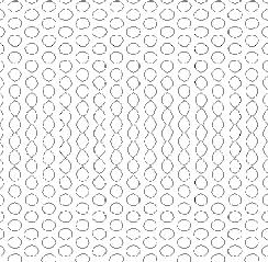
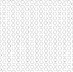
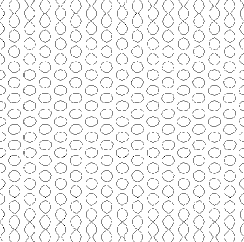
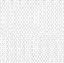
FIG. 11.: A real-space illustration of the stable oscillations of the perturbation mode for $R=0.0355$, $k=1.02$, $\alpha=0.1$, $\beta=0$, $\gamma=6$, $g_{2}=0$ at times $t=0$, $t=50$, $t=110$, $t=170$. Indicated in the figure are the zero level contours of the solution.

When the wavenumber $k$ or the control parameter $R$ is increased beyond the line marked by diamonds in Fig.6b the modulated hexagons become unstable and the regular pattern breaks down leading to a temporally and spatially chaotic state. Typical snapshots are displayed in Fig.12a,b. They suggest a strong signature of a hexagonal symmetry and a predominant orientation of the disordered pattern which rotates in time. This is brought out more clearly in the power spectrum of Fig.12a pictured in Fig.12c, which clearly shows six dominant peaks (see also Fig.15 below). Its temporal evolution is depicted in Fig.13a as a space-time diagram of the radially integrated power spectrum Fig.12c with time increasing upward. Since $\psi$ is real, only the range $-90^{o}$ to $90^{o}$ is shown. The rotation of the spectrum is seen to be surprisingly pronounced and steady over long periods of time, which are intermittently interrupted by periods during which the peaks in the spectrum are less pronounced. The space-time autocorrelation function of this state as obtained from a run of duration $T_{max}=278,880$ is shown in Fig.13b. The azimuthal decay of the correlation function is seen to be quite slow. We do not expect that the sixfold symmetry of the power spectrum persists as the system size is increased. In fact, the highest peaks in the power spectrum decrease by roughly a factor of two if the linear dimensions of the system are doubled. However, Fig.13a,b indicates that the disordered state at least locally exhibits a structure with hexagonal symmetry, which rotates in time.

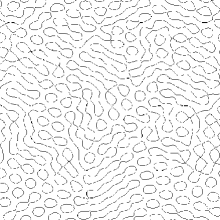
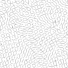
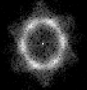
FIG. 12.: a) Zero-level contours in real space for time $t=118580$. b) Zero-level contours at a time when the power spectrum has rotated by about $30^{o}$. c) Power spectrum on a logarithmic scale of pattern at time $t=118580$ for $\alpha=0.1$, $\gamma=6$, $R=0.036$, $k=1.02$. Note the residual sixfold symmetry.

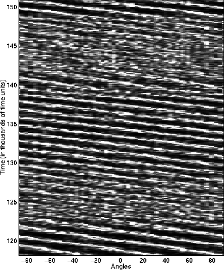
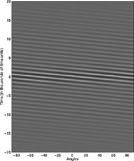
FIG. 13.: Temporal evolution of radially integrated power spectrum and space-time correlation thereof in the disordered domain $\alpha=0.1$, $\gamma=6$, $R=0.036$, $k=1.02$ (cf. Fig.10).

The modulated hexagons and the disordered hexagons shown in Fig.11 and Fig.12 are obtained in the minimal model (2) and arise from the short-wave instability connected with the translation mode. Very similar results are also obtained in the more general model (3) where they can also arise from the short-wave Hopf mode. For the nonlinear evolution the long-wave behavior of the branch of destabilizing modes is apparently not relevant.

An interesting aspect of the disordered state of Fig.12 is that it exists stably for the same value of the control parameter as the steady hexagons and the modulated hexagons. This coexistence of ordered and disordered states is reminiscent of the situation in Rayleigh-Bénard convection with small Prandtl number where the state of spiral-defect chaos coexists with that of straight parallel rolls [2].

It is less surprising to find complex dynamics in parameter regimes in which no stable steady hexagons exist. Such a case is shown in Fig.14. The parameters are as in Fig.6c with $R$ (marked by a line in Fig.6c) chosen in the gap between the stable steady hexagons and the transition line to unmodulated oscillating hexagons. In this case the disorder is sufficiently strong that the power spectrum is essentially isotropic for the system sizes investigated.

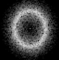
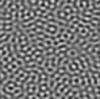
FIG. 14.: Power spectrum on a logarithmic scale and zero-level contour lines of real space of disordered state at $\alpha=0.1$, $\gamma=14$, $R=0.052$, at time $t=22400$ in the minimal model (cf. Fig.6c).

From an experimental point of view an important question is whether the interesting dynamic states identified here are actually accessible even if the initial conditions cannot be prepared carefully. After all, they occur in parameter regimes in which the system could also evolve into a stripe pattern. We have therefore performed a few simulations starting from random initial conditions. For the parameters in the stability gap of Fig.6c the system evolves directly to a disordered state like that shown in Fig.14. Fig.15 shows the space-time diagram for a simulation starting from small random initial conditions for parameter values for which steady and modulated hexagons coexist stably with the disordered state (cf. Fig.12). Clearly, the spectrum is initially essentially isotropic (bottom panel), reflecting the random initial conditions, and then evolves into a more ordered spectrum (top panel) corresponding to the rotating state discussed above. These runs suggest that the states found here should be experimentally accessible. Of course, so far no information is available to what extent the Swift-Hohenberg models discussed here describe a concrete physical system and whether the parameter regimes in which the dynamical states arise are accessible experimentally.

FIG. 15.: Temporal evolution of radially integrated power spectrum starting from random initial conditions for $\alpha=0.1$, $\gamma=6$, $R=0.03$ (cf. Fig.10).

V Conclusion

Motivated by the Küppers-Lortz instability of roll patterns in the presence of rotation we have investigated the effect of rotation on the stability of hexagonal patterns. To get a first impression we have studied a minimal and a more general Swift-Hohenberg-type order-parameter model. In a linear stability analysis of the weakly nonlinear hexagon pattern we focussed on instabilities that lead out of the space spanned by the modes corresponding to the hexagons themselves. Long- and short-wave instabilities were found, which can be steady or oscillatory. Immediately at onset the wavenumber band is limited by an instability arising from the translation mode. For larger rotation rates it may be oscillatory. In contrast to the case of roll patterns in the presence of rotation, which for sufficiently large rotation rates can become unstable at all wavenumbers immediately at onset due to the Küppers-Lortz instability, no such parameter range is found for the hexagons.

Further above threshold the instabilities typically become short-wave and oscillatory. They can lead to periodically oscillating spatially modulated hexagons or to a disordered state characterized by cellular and stripe-like elements. Locally the structure can exhibit a surprisingly regular rotation of the orientation of its residual hexagonal symmetry. It is worth comparing this behavior with that arising in the Küppers-Lortz regime of systems with up-down symmetry. While in numerical simulations of an order-parameter model a very pronounced switching between the three orientations of the stripe pattern was found [11], in experiments also a behavior was observed that is more akin to the rotation of the spectrum found here [8]. Particularly striking is the fact that the disordered state found here can arise for the same control parameter value as the periodically oscillating modulated hexagons and the steady hexagons. This apparent stable coexistence of the spatio-temporally chaotic state with an ordered state is reminiscent of the spiral-defect chaos found in Rayleigh-Bénard convection, which coexists with the straight-roll state [34]. An interesting question is whether propagating fronts separating the ordered from the disordered state can be found as has been in those experiments.

In investigations of the stability of hexagons with broken chiral symmetry within the framework of coupled Ginzburg-Landau equations the same type of long- and short-wave, steady and oscillatory instabilities have been identified recently [35]. There also a regime was found in which the instability does not lead to an ordered state although such a state is stable for the same value of the control parameter. In the Ginzburg-Landau equations, however, that state cannot be described appropriately. They break the isotropy of the system and can only describe perturbations that make a small angle with respect to the hexagon pattern. Since the disordered state that was found in the Swift-Hohenberg equations investigated here exhibits an almost isotropic Fourier spectrum (cf. Figs.12,14), it leads to the excitation of ever higher Fourier modes in the numerical simulation of the Ginzburg-Landau equations. This renders them useless for the investigation of the chaotic state.

In order to make concrete predictions for experimental systems the order-parameter equations have to be derived for specific physical systems. Situations of interest are Marangoni convection and Rayleigh-Bénard convection with broken Boussinesq symmetry. For Marangoni convection with poorly conducting boundaries [25, 33] the effect of rotation has only been included recently in the derivation of long-wave equations [32]. The case of Rayleigh-Bénard convection has been treated to some extent. For poorly conducting boundaries a systematic long-wave expansion has been performed [24]. By imposing asymmetric boundary conditions (but neglecting other non-Boussinesq effects) quadratic terms in the order parameter equation were obtained, including the crucial term involving $\gamma$ that breaks the chiral symmetry. In that work the analysis focused on square rather than hexagonal patterns [24].

If the pattern arises first at a finite (i.e. not small) wavenumber an equation of the form (2) or (3) can be obtained in an approximation in which the kernel of the nonlinear integral term in Fourier space is approximated by local terms in real space [30, 20, 31]. For Boussinesq Rayleigh-Bénard convection with and without rotation it has been found that such an approximation can yield good agreement with weakly nonlinear amplitude equations while still preserving the isotropy of the system [19]. The non-Boussinesq case with rotation has not been treated yet.

We gratefully acknowledge helpful discussions with B. Echebarria, A. Golovin, A. Mancho, W. Pesch, and M. Silber. The computations were done with a modification of a code by G. D. Granzow. This work was supported by D.O.E. Grant DE-FG02-G2ER14303 and NASA Grant NAG3-2113.

REFERENCES

- [1] J. Swift, in Contemporary Mathematics Vol. 28 (American Mathematical Society, Providence, 1984), p. 435.
- [2] S. Morris, E. Bodenschatz, D. Cannell, and G. Ahlers, Phys. Rev. Lett. 71, 2026 (1993).
- [3] W. Decker, W. Pesch, and A. Weber, Phys. Rev. Lett. 73, 648 (1994).
- [4] G. Küppers and D. Lortz, J. Fluid Mech. 35, 609 (1969).
- [5] F. Busse and K. Heikes, Science 208, 173 (1980).
- [6] R. May and W. Leonard, SIAM J. Appl. Math. 29, 243 (1975).
- [7] F. Zhong, R. Ecke, and V. Steinberg, Physica D 51, 596 (1991).
- [8] Y. Hu, R. Ecke, and G. Ahlers, Phys. Rev. Lett. 74, 5040 (1995).
- [9] Y. Hu, R. Ecke, and G. Ahlers, Phys. Rev. E 55, 6928 (1997).
- [10] Y. Tu and M. Cross, Phys. Rev. Lett. 69, 2515 (1992).
- [11] M. Cross, D. Meiron, and Y. Tu, Chaos 4, 607 (1994).
- [12] H. Xi, J. Gunton, and G. Markish, Physica A 204, 741 (1994).
- [13] N. Tufillaro, R. Ramshankar, and J. Gollub, Phys. Rev. Lett. 62, 422 (1989).
- [14] A. Kudrolli and J. Gollub, Physica D 97, 133 (1996).
- [15] Q. Ouyang and H. Swinney, Chaos 1, 411 (1991).
- [16] A. Soward, Physica D 14, 227 (1985).
- [17] J. Millàn-Rodriguez et al., Phys. Rev. A 46, 4729 (1992).
- [18] J. Swift and P. Hohenberg, Phys. Rev. A 15, 319 (1977).
- [19] M. Neufeld, R. Friedrich, and H. Haken, Z. Phys. B 92, 243 (1993).
- [20] M. Bestehorn and R. Friedrich, in A Perspective Look at Nonlinear Media, edited by J. Parisi, S. Müller, and W. Zimmermann (Springer, Berlin, 1998), p. 31.
- [21] C. Kubstrup, H. Herrero, and C. Perez-Garcia, Phys. Rev. E 54, 1560 (1996).
- [22] H. Sakaguchi and H. Brand, J. Phys. II 7, 1325 (1997).
- [23] C. Crawford and H. Riecke, Physica D 129, 83 (1999).
- [24] S. Cox, SIAM J. Appl. Math. 58, 1338 (1998).
- [25] E. Knobloch, Physica D 41, 450 (1990).
- [26] M. Bestehorn, Phys. Rev. E 48, 3622 (1993).
- [27] M. Sushchik and L. Tsimring, Physica D 74, 90 (1994).
- [28] D. Riahi, Int. J. Eng. Sci. 32, 877 (1994).
- [29] H. Sakaguchi and H. Brand, Physica D 97, 274 (1996).
- [30] H. Haken, Advanced Synergetics : Instability Hierarchies of Self- Organizing Systems and Devices (Springer-Verlag, Berlin, 1983).
- [31] M. Bestehorn and R. Friedrich, Phys. Rev. E 59, 2642 (1999).
- [32] A. Mancho, F. Sain, and H. Riecke, unpublished .
- [33] V. Gertsberg and G. Sivashinsky, Prog. Theor. Phys. 66, 1219 (1981).
- [34] R. Cakmur, D. Egolf, B. Plapp, and E. Bodenschatz, Phys. Rev. Lett. 79, 1853 (1997).
- [35] B. Echebarria and H. Riecke, submitted to Physica D. .