A Transverse Oscillation Arising From Spatial Soliton Formation in Nonlinear Optical Cavities

Abstract

A new type of transverse instability in dispersively nonlinear optical cavities, called the optical whistle, is discussed. This instability occurs in the mean field, soliton forming limit when the cavity is driven with a finite width Gaussian beam, and gives rise to oscillation, period doubling, and chaos. It is also seen that bistability is strongly affected due to the oscillation within the upper transmission branch. The phenomenon is interpreted as a mode mismatch in the soliton formation process and is believed to have broad applicability.

Introduction

Over the last 25 years the nonlinear optical resonator has been a rich source of interesting phenomena [1]. These systems are attracting attention recently due to their potential applications as all-optical switches, memories [2], and logic gates [3], at both the classical and quantum levels. The resonator geometry naturally gives appreciably stronger nonlinear effects for a given incident beam intensity than do the travelling wave schemes, potentially allowing the use of faster, less lossy, materials with relatively weaker nonlinearities (for example, atomic vapors or even silica as opposed to thermal or photorefractive materials). The resonator geometry also leads to a variety of time-dependent behaviors which must be adequately characterized, either to avoid undesired effects in engineered systems or to perhaps take advantage of them for communications or computing purposes.

The most fundamental physical process in the nonlinear resonator, plane wave optical bistability, was first observed experimentally in 1975 [4]. Ikeda [5] later showed in a discrete return-map analysis that as the incident intensity increases the intracavity field intensity can oscillate and undergo a period doubling route to chaos. In the 1980’s a great deal of work concentrated on transverse structure and dynamics in nonlinear cavities, in order to incorporate the phenomena of self-(de)focusing and diffraction. McLaughlin et al [6] demonstrated in 1985 that a finite-width Gaussian beam incident on a cavity with a single transverse dimension can give rise to a transverse oscillation in the cavity field, essentially due to a modulational instability. These oscillations are of period equal to a multiple of the cavity round-trip time and thus correspond to the occupation of multiple resonator longitudinal modes. More recently Haelterman and Vitrant discussed a transverse oscillation which arises when a nonlinear Fabry-Perot is illuminated obliquely, due to the lateral drift of the field within the cavity [7].

Here we report on the discovery of a new type of oscillation within high-finesse nonlinear cavities driven by Gaussian beams. This optical whistle oscillation occurs as a competition between spatial soliton formation [8][9] and the driving input, and can exhibit oscillatory or chaotic behavior.

General Considerations

The dynamics of a general (dispersively) nonlinear optical cavity driven with a finite-width beam is principally governed by four effects: propagation, damping, diffraction, and nonlinearity. A qualitative understanding of cavity behavior is gained by simply comparing the characteristic timescales of these processes, given by:

$$\begin{array}[]{rcl}\tau_{prop}&=&L/c\\ \tau_{damp}&=&L{\cal F}/c\\ \tau_{diff}&=&w^{2}/\lambda c\\ \tau_{nl}&=&\lambda/c\Delta n\end{array}$$ (1)

where $L$ and $\cal F$ are the cavity length and finesse, $\lambda$ is the optical wavelength, $w$ is a characteristic size of transverse features in the optical beam, and $\Delta n=|n(I)-n(0)|$ is the typical nonlinear index shift caused by the optical field of typical intensity $I$ (the linear index is assumed to be unity).

The timescale $\tau_{nl}$ is the time required for the nonlinearity to induce a $2\pi$ phase shift in the light field. For self-focusing nonlinearities we can also identify $\tau_{nl}$ as the typical formation time of transverse structure arising from the modulational instability [10]. These structures form with characteristic transverse wavelength $\Lambda=\lambda/\sqrt{\Delta n}$. A feature of this size will diffract apart in a time $\Lambda^{2}/(\lambda c)\approx\tau_{nl}$, and we generally conclude that these structures spontaneously form so that diffraction and nonlinearity are equally important. The same result applies to the formation of spatial solitons, which can be considered modes of self-induced waveguides [11][12]. Soliton formation is more efficient when the incident beam is of size $\Lambda$, in analogy with mode-matching in linear optics. The optical whistle instability arises from a “mode mismatch” between the incident beam size and the (self-consistent) soliton dimension $\Lambda$.

Returning to the cavity timescales of Eq. 1, one important case is when $\tau_{prop}$ is much shorter than the others. In this mean field limit the field changes little in traversing the cavity once, and we can suppress the field envelope’s longitudinal dependence. It can be shown that in this limit only a single longitudinal cavity mode is appreciably occupied [13].

The optical whistle phenomenon exists under the same conditions as spatial soliton formation:

$$\tau_{prop}\ll\tau_{diff}\approx\tau_{nl}\ll\tau_{damp}$$ (2)

For the remainder of the discussion we confine ourselves to this case. From Eq. 1 it follows that we are discussing a high-finesse cavity.

The Nonlinear Cavity Equation

We now restrict our attention to a Kerr nonlinear cavity having a single transverse degree of freedom $x$. The cavity’s internal field envelope is governed by the Lugiato-Lefever equation [14], written here as

$$\frac{\partial{\cal E}}{\partial t}=\frac{ic}{2k}\frac{\partial^{2}{\cal E}}{\partial x^{2}}-\Gamma^{\prime}{\cal E}+i(\Delta\omega^{\prime}){\cal E}+\Gamma^{\prime}{\cal E}_{drive}+i\omega n_{2}|{\cal E}|^{2}{\cal E}\,,$$ (3)

where ${\cal E}$ is the internal cavity field envelope amplitude, $k=2\pi/\lambda$ is the longitudinal wavenumber, $\Gamma^{\prime}=cT/L$ is the amplitude decay rate from the cavity ($T$ is the amplitude transmission coefficient at each mirror, assumed equal, and $L$ is the cavity length), $\omega$ is the field angular frequency, $\Delta\omega^{\prime}=\omega-\omega_{cav}$ is the detuning of the driving field from linear cavity resonance, and $n_{2}$ is the nonlinear index inside the cavity. A time-independent version of this equation was also derived by Haelterman et al from their modal theory [15]. Equation 3 is slightly different from the version in Ref. [14], which has been rescaled to yield $\Gamma=1$; here we will employ a different rescaling to easily accomodate the important limit $\Gamma\rightarrow 0$.

Equation 3 is now made dimensionless by choosing an arbitrary distance scale $x_{0}$ and relating the time and field scales $t_{0}$ and $|{\cal E}_{0}|$ to it using $t_{0}=kx_{0}^{2}/c$ and $|{\cal E}_{0}|=1/{kx_{0}\sqrt{|n_{2}|}}$. After rescaling Eq. 3 takes on the dimensionless form

$$\dot{\Psi}=\frac{i}{2}\nabla^{2}\Psi+i\eta|\Psi|^{2}\Psi+i\Delta\omega\Psi-\Gamma(\Psi-\Psi_{drive})\,,$$ (4)

where $\eta=+1(-1)$ for self-focusing (-defocusing), $\Psi={\cal E}/|{\cal E}_{0}|$, $\Delta\omega=\Delta\omega^{\prime}t_{0}$, and $\Gamma=\Gamma^{\prime}t_{0}$. The conditions of Eq. 2 have allowed us to use the mean field limit in deriving this equation and also imply that $\Gamma\ll 1$.

Soliton Filtering and the Optical Whistle

Equation 4 is a damped, driven version of the nonlinear Schrödinger equation. In the limit $\Gamma\rightarrow 0$ and for $\eta=+1$ it admits the family of stationary soliton solutions [16]

$$\begin{array}[]{rcl}\Psi(X,T)&=&d^{-1}\,{\mathrm{s}ech}(X/d)\\ \Delta\omega&=&-1/(2d^{2})\end{array}$$ (5)

where $d$ is an arbitrary width and $X=x/x_{0}$, $T=t/t_{0}$ are dimensionless coordinates. There are other, time-dependent (“breather”), soliton solutions [17] which are unimportant for our present purposes. Equation 5 is also a solution in the damped case ($\Gamma\neq 0$) if the driving field has the special form

$$\Psi_{drive,sech}(X,T)=\Psi(X,T)=d^{-1}\,{\mathrm{s}ech}(X/d)\,.$$ (6)

Whether this $\Gamma\neq 0$ solution is a soliton in the mathematical sense is a subtle issue and not resolved here. We will take the common practical approach and refer to this as a “soliton solution” in reference to its observed soliton-like robustness, keeping in mind the potential inappropriateness of this terminology.

A general qualitative feature of solitons is their robustness to small perturbations. Hence we might expect that the Gaussian driving field

$$\Psi_{drive,Gaussian}(X,T)=d^{-1}\,{\mathrm{e}xp}\left[-X^{2}/(1.699d)^{2}\right]\,.$$ (7)

may lead to the soliton solution (5) nearly as efficiently as the sech drive (6) when $\Gamma\ll 1$. The constant 1.699 has been chosen to minimize the difference integral

$$\int_{-\infty}^{\infty}\left[\Psi_{drive,Gaussian}(X)-\Psi_{drive,sech}(X)\right]^{2}\,dx\,.$$ (8)

This possibility was considered in a travelling wave geometry by Burak and Nasalski [18], who found that as much as 99.5% of the incident power is converted into a soliton.

In our present situation it is found that the folded path arising from the cavity configuration can modify this picture substantially. Generally, soliton forming behavior is observed when the driving field amplitude is matched to its width, as in Eq. 7. Because the non-sech incident beam profile yields a sech beam in transmission, we call this process soliton filtering in analogy with ordinary spatial filtering. A larger driving amplitude leads to a “mode mismatch” since the soliton is trying to form with a smaller width than the input beam. The optical whistle oscillation results from a competition between the soliton trying to shrink in size, and the driving field feeding in light mismatched in phase and spatial profile.

Considering again the Gaussian driving field of Eq. 7, recall that the choice of distance scale $x_{0}$ in deriving Eq. 4 is arbitrary, so we can choose it to be the waist size of the input beam without loss of generality. (In this case the time scale $t_{0}$ is the time of flight through the beam’s Rayleigh range.) Then we have $\Psi_{drive}(X,T)=q\,\exp{(-X^{2})}$ where $q$ is a real, dimensionless driving amplitude, and our model is characterized by the four real dimensionless quantities $\eta$, $\Gamma$, $\Delta\omega$, and $q$. We expect optimal coupling into the soliton when

$$\begin{array}[]{rcl}q&\approx&1.699\\ \Delta\omega&\approx&-(1.699)^{2}/2=-1.443\,.\\ \end{array}$$ (9)

The former is remarkably close to the optimal value $1.69$ in the travelling wave case, found using the inverse scattering transform [18].

Numerical Results

Equation 4 is solved using a version of the popular split-step technique [19][20], accurate through two orders in the time step size $h$. The results presented below are calculated using $h=0.01$ and a spatial grid consisting of 256 points separated by 0.156 dimensionless units. These values are found to give accurate results for the cases of interest here; halving the grid spacings in space and time yields essentially identical results for a variety of test cases.

Oscillation

Figure 1 summarizes the asymptotic (long-time) cavity solutions when the Gaussian driving field is suddenly turned on at $t=0$. We have here assumed an initially empty cavity, $\eta=+1$, and $\Gamma=0.14$. The asymptotic cavity solutions are categorized into five basic types: (1) steady state solutions, (2) period 1 oscillations, (3) period 2 oscillations, (4) long period oscillations, and (5) chaos. The regions are seen to have complex boundaries, and points near the borders of the “chaotic” regions show particularly interesting behaviors: at the borders with steady state regions lie oscillations of very long period, and at the borders with the normal oscillating regions period doubling occurs. Period 3 oscillations are also observed.

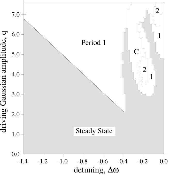
FIG. 1.: Asymptotic behavior of cavity field, for $\eta=+1$, $\Gamma=0.14$, and an initially empty cavity. Labels indicate regions of steady state, period 1 oscillation (1), period 2 oscillation (2), and chaos (C).

Time series of examples are shown in Figure 2, where we plot the total power output for a variety of cases. For the period 1 example, snapshots of the cavity field amplitude are shown in Figure 3. The field profile narrows as the soliton forms, then is attenuated as the nonlinearity shifts the peak out of cavity resonance and power enters at the edges. The fundamental oscillation frequencies for several cases are plotted in Figure 4. It is not known what ranges of $\Gamma$ permit oscillations to occur.

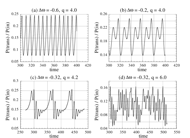
FIG. 2.: Time series of transmitted power for specified parameters, illustrating the asymptotic solutions shown in Fig. 1. (a) period 1, (b) period 2, (c) long period, and (d) chaotic oscillation. $\eta=+1$, $\Gamma=0.14$.

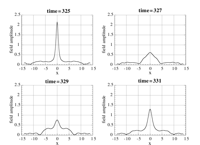
FIG. 3.: Cavity field amplitude profiles for the period 1 oscillation shown in Figure 2(a). $\Delta\omega=-0.6$, $q=4.0$,$\Gamma=0.14$.

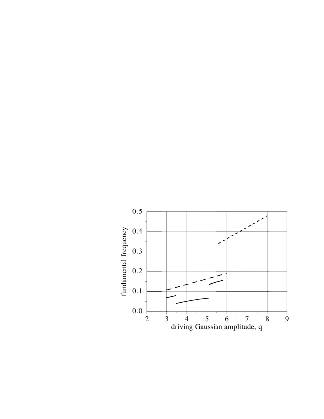
FIG. 4.: Fundamental frequency of oscillation as a function of driving amplitude $q$. The solid curve is for $\Gamma=0.14$, $\Delta\omega=-0.2$ and shows one of the period-doubled regions of Fig. 1. The long dashed curve is for $\Gamma=0.14$, $\Delta\omega=-0.6$. The short dashed curve is for $\Gamma=0.3$, $\Delta\omega=-0.6$.

Bistability

An interesting issue is the effect the optical whistle has on dispersive optical bistability. Figure 5 compares a bistability curve from our time-dependent analysis with that given in Ref. [21] which assumed a steady state field. Our respective equations have been made dimensionless in slightly different manners; to correspond to the $X_{0}=1$, $\Delta=+3$ curve in their Figure 3a we have chosen $\Gamma=X_{0}^{2}/2=0.5$, $\Delta\omega=-\Gamma\Delta=-1.5$ and have related their field amplitude $f$ to ours using $\Psi=\sqrt{\Gamma}f$. Part of the upper branch of the bistability curve is seen to be unstable due to the whistle oscillation, and the oscillation amplitude is indicated by the bars in Fig. 5. In general we observe that where bistability occurs ($\Delta\omega<-0.19$ for $\Gamma=0.14$) the whistle oscillation occurs only in the upper branch of the bistability curve. However, the oscillation can also occur when there is no bistability, as is evident from Fig. 1.

FIG. 5.: Comparison with steady state theory. The dashed bistability curve is from Fig. 3a of Vitrant et al (1990) and the solid curve is from our time-dependent analysis. Bars on the solid curve show the oscillation amplitude. $\Gamma=0.5$, $\Delta\omega=-1.5$.

In other cases the optical whistle modifies bistability curves more dramatically. Figure 6 shows steady state and time-dependent bistability curves for $\Gamma=0.14$, $\Delta\omega=-1.443$. In this case the whistle oscillation has moved the switch-off point substantially, a common occurrence. In contrast, the switch-on point has not been seen to change from its steady state value in our analysis.

FIG. 6.: Comparison of steady state (dashed) and time-dependent (solid, with oscillation amplitude indicated by bars) analyses. In this case the whistle instability changes the switch-off point in the bistability curve. $\Gamma=0.14$, $\Delta\omega=-1.443$.

Soliton Formation

We argued above that the soliton solution of Eq. 5 would be stable when $\Gamma\ll 1$, in the sense that a sech-profiled cavity field would result when a Gaussian driving beam is applied. This is numerically demonstrated in Figure 7 where steady state field solutions are presented for the cases $\Gamma=0.1$ and $\Gamma=10$. The former solution is very close to the sech form of Eq. 5, and the latter is close to the Gaussian driving field. Although the existence of solitons in a damped cavity is an unresolved technical question, the sech solutions are seen to be quite stable when $\Gamma\ll 1$.

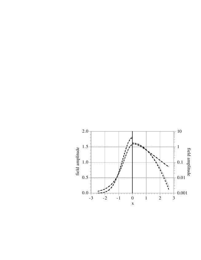
FIG. 7.: Steady state field solution with Gaussian drive, plotted on linear and logarithmic scales, in the upper transmission branch. The dashed curves are the driving function and $1.58\,\mathrm{sech}(1.575x)$; overlapping solid curves are solutions with $\Gamma=10$ and $\Gamma=0.1$, respectively. The latter solution is very close to the soliton form of Eq. 5 despite being driven by a Gaussian beam, providing evidence for the stability of the sech solution when $\Gamma\ll 1$. $q=1.8$, $\Delta\omega=-1.2$.

In the travelling wave case soliton formation with Gaussian driving beams can be very efficient; as much as 99.5% of the input power can be transformed into a soliton [18]. In a cavity we might expect this to be an upper bound since imperfect interference (and reflection of the incident beam) would seem to present an additional loss of efficiency. In Eq. 9 we made a simple estimate of the optimal coupling parameters. However, Fig. 6 shows that for $\Delta\omega=-1.443$, $\Gamma=0.14$ the whistle disrupts the bistability curve’s upper branch near $q=1.699$. A nearby case ($\Delta\omega=-1.2$, $\Gamma=0.14$) without the disruption is shown in Fig. 8. At the switch-off point $q\approx 1.6$ the coupling efficiency into the transmitted beam is 97.6%, still quite high. Because $\Gamma=0.14\ll 1$ the transmitted field is found to be quite close to the sech form of Eq. 5; when $\Gamma>1$ the transmitted field is more Gaussian in profile. Figure 9 shows the steady state soliton width in the upper branch of Fig. 8, and the decrease in width as the oscillation point is reached. For the present work we have not attempted a thorough study to optimize soliton coupling efficiency but wish to point out that fairly high efficiencies are possible in cavities.

FIG. 8.: Bistability curve showing nearly complete (97.6%) coupling into the transmitted sech beam. The expected optimal case, Eq. 9, is disrupted by the whistle as shown in Fig. 6. $\Delta\omega=-1.2$, $\Gamma=0.14$.

FIG. 9.: Width $d$ of soliton solution in upper branch of Fig. 8 as a function of driving amplitude $q$. As $q$ increases the soliton narrows in width and begins oscillating at $q\approx 2.4$. $\Delta\omega=-1.2$, $\Gamma=0.14$.

Discussion

A variety of instability phenomena similar to the optical whistle have been reported in the literature [1]. These can be broadly categorized into multi-mode and single-mode (mean field) effects. In the former case the plane wave oscillation phenomenon has been called “self-pulsing” (it occurs in both the context of absorptive [22] and dispersive [5][23] bistability). The instability here is essentially due to the interplay of two different timescales, nonlinearity and cavity feedback, and gives rise to an oscillation period which is a multiple of the cavity round-trip time. Slightly later the single-mode case was also shown to yield oscillations. Ikeda and Akimoto [24] first demonstrated this within a plane wave, purely dispersive Kerr model. Lugiato et al [25] constructed a more realistic optical Bloch model and found oscillations (and chaos) in that case as well, again at the plane wave level of description.

Our work is more closely related to the transverse instability discovered by McLaughlin et al [26] and discussed in the mean field limit by Lugiato and Lefever [14]. In these studies, stationary transverse structure in a broad illuminating beam arises from a modulational instability. McLaughlin et al [6] showed in 1985 that the transverse features can oscillate in time. In all cases, more recent numerical work has shown that these transverse perturbations can grow to become soliton chains [7][27] which may or may not be stationary in time. Lastly, for a plane wave driving field of variable intensity a series of bifurcations similar to the ones seen here are observed to occur in the mean field case, eventually leading to spatio-temporal chaos [28]. Our present work is different from these earlier results because here the most unstable transverse wavelength is comparable to the driving field width; the instability consists of a broad spectrum of transverse wavenumbers and it is somewhat more intuitive to view the process as a mode mismatch in the soliton formation process rather than as a sinusoidal modulation in a very broad beam growing into a (perhaps) time-varying soliton chain.

There are several possible experimental configurations in which the optical whistle might be observed. One concrete realization is a fiber-loop geometry [29], in which Gaussian pulses from a laser are injected into a (nonlinear) fiber loop and the copropagating longitudinal coordinate $z-vt$ plays the role of the tranverse dimension $x$ in our analysis. Another possibility is a cylindrical nonlinear cavity with strong single-moding in the $y$ and $z$ dimensions [30].

The optical whistle phenomenon presented here is believed to exist beyond the Kerr nonlinear, one dimensional model, whenever one is in the soliton forming limit of Eq. 2. We conjecture this on the basis of our general picture that the whistle is the result of a mode mismatch between the generated soliton and driving field. The study of related phenomena in other systems would be an interesting topic of further research.

REFERENCES

- [1] For a comprehensive review see R. Reinisch and G. Vitrant, Prog. Quant. Electr. 18, 1 (1994).
- [2] W.J. Firth and A.J. Scroggie, Phys. Rev. Lett. 76, 1623 (1996).
- [3] Q.A. Turchette, C.J. Hood, W. Lange, H. Mabuchi, and H.J. Kimble, Phys. Rev. Lett. 75, 4710 (1995).
- [4] S.L. McCall, H.M. Gibbs, G.G. Churchill, and T.N.C. Venkatesan, Bull. Am. Phys. Soc. 20, 636 (1975); S.L. McCall, H.M. Gibbs, and T.N.C. Venkatesan, J. Opt. Soc. Am. 65, 1184 (1975).
- [5] K. Ikeda, Opt. Comm. 30, 257 (1979).
- [6] D.W. McLaughlin, J.V. Moloney, and A.C. Newell, Phys. Rev. Lett. 54, 681 (1985).
- [7] M. Haelterman and G. Vitrant, J. Opt. Soc. Am. B 9, 1563 (1992).
- [8] R.Y. Chiao, E. Garmire, and C.H. Townes, Phys. Rev. Lett. 13, 479 (1964).
- [9] S.A. Akhmanov, A.P. Sukhorukov, and R.V. Khokhlov, Sov. Phys. JETP 23, 1025 (1966).
- [10] T.B. Benjamin and J.E. Fier, J. Fluid Mech. 27, 417 (1966).
- [11] A.W. Snyder, D.J. Mitchell, and Yu.S. Kivshar, Mod. Phys. Lett. B 9, 1479 (1995).
- [12] A.W. Snyder and Yu.S. Kivshar, J. Opt. Soc. Am. B 14, 3025 (1997).
- [13] L.A. Lugiato and L.M. Narducci, Z. Phys. B 71, 129 (1988).
- [14] L.A. Lugiato and R. Lefever, Phys. Rev. Lett. 58, 2209 (1987).
- [15] M. Haelterman, G. Vitrant, and R. Reinisch, J. Opt. Soc. Am. B 7, 1309 (1990).
- [16] R.Y. Chiao, I.H. Deutsch, J.C. Garrison, and E.W. Wright, in Frontiers in Nonlinear Optics: the Serge Akhmanov Memorial Volume, edited by H. Walther, N. Koroteev, and M.O. Scully (Institute of Physics Publishing, Bristol and Philadelphia, 1993), p. 151.
- [17] G.P. Agrawal, Nonlinear Fiber Optics (Academic Press, San Diego, 1989), p. 111.
- [18] D. Burak and W. Nasalski, Applied Optics 33, 6393 (1994).
- [19] Ref. [17], p. 44.
- [20] T.R. Taha and M.J. Ablowitz, J. of Comp. Phys. 55, 203 (1984).
- [21] G. Vitrant, M. Haelterman, and R. Reinisch, J. Opt. Soc. Am. B 7, 1319 (1990).
- [22] R. Bonifacio, M. Gronchi, and L.A. Lugiato, Opt. Comm. 30, 129 (1979).
- [23] L.A. Lugiato, Opt. Comm. 33, 108 (1980).
- [24] K. Ikeda and O. Akimoto, Phys. Rev. Lett. 48, 617 (1982).
- [25] L.A. Lugiato, L.M. Narducci, D.K. Bandy, and C.A. Pennise, Opt. Comm. 43, 281 (1982).
- [26] D.W. McLaughlin, J.V. Moloney, and A.C. Newell, Phys. Rev. Lett. 51, 75 (1983).
- [27] G.S. McDonald and W.J. Firth, J. Opt. Soc. Am. B 7, 1328 (1990).
- [28] K. Nozaki and N. Bekki, Physica 21D, 381 (1986).
- [29] A. Schwache and F. Mitschke, Phys. Rev. E 55, 7720 (1997).
- [30] I.H. Deutsch and R.Y. Chiao, Phys. Rev. Lett. 69, 3627 (1992).