Simple and Superlattice Turing Patterns in Reaction-Diffusion Systems: Bifurcation, Bistability, and Parameter Collapse

Abstract

We use equivariant bifurcation theory to investigate pattern selection at the onset of a Turing instability in a general two-component reaction-diffusion system. The analysis is restricted to patterns that periodically tile the plane in either a square or hexagonal fashion. Both simple periodic patterns (stripes, squares, hexagons, and rhombs) and “superlattice” patterns are considered. The latter correspond to patterns that have structure on two disparate length scales; the short length scale is dictated by the critical wavenumber from linear theory, while the periodicity of the pattern is on a larger scale. Analytic expressions for the coefficients of the leading nonlinear terms in the bifurcation equations are computed from the general reaction-diffusion system using perturbation theory. We show that, no matter how complicated the reaction kinetics might be, the nonlinear reaction terms enter the analysis through just four parameters. Moreover, for hexagonal problems, all patterns bifurcate unstably unless a particular degeneracy condition is satisfied, and at this degeneracy we find that the number of effective system parameters drops to two, allowing a complete characterization of the possible bifurcation results at this degeneracy. For example, we find that rhombs, squares and superlattice patterns always bifurcate unstably. We apply these general results to some specific model equations, including the Lengyel-Epstein CIMA model, to investigate the relative stability of patterns as a function of system parameters, and to numerically test the analytical predictions.

1 Introduction

Regular patterns arise in a wide variety of physical, chemical and biological systems that are driven from equilibrium. The origin of these spatial patterns can often be traced to a symmetry-breaking instability of a spatially-homogeneous state. Such an instability mechanism was proposed by Alan Turing in 1952 [1] for pattern formation in chemical systems featuring both reaction and diffusion. The key insight of Turing was that diffusion, which is usually thought of as a stabilizing mechanism, can actually act as a destabilizing mechanism of the spatially-uniform state. This is the case, for example, in a class of two-component activator-inhibitor systems, provided the inhibitor diffuses more rapidly than the activator. This competition between long-range inhibition and short-range activation can lead to spatially inhomogeneous steady states called Turing patterns [2]. Experimental evidence of Turing patterns was discovered only recently[3], and a number of experiments on the Turing instability have now been carried out on the chlorite-iodide-malonic acid (CIMA) reaction in a gel [3, 4, 5]. These experiments have demonstrated the existence and stability of a variety of regular patterns, including stripes, hexagons, and rhombs. At the same time, a two variable model of the CIMA reaction has been proposed by Lengyel and Epstein [6].

Equivariant bifurcation theory [7] is a powerful tool for analyzing the nonlinear evolution of symmetry-breaking instabilities in pattern-forming systems. This approach determines the generic behaviors associated with bifurcation problems that are equivariant with respect to a given group of linear transformations. In particular, the form of the bifurcation problem is restricted by symmetry considerations, limiting the behavior to some finite set of possibilities. The problem of determining which type of behavior occurs in a given physical system then reduces to one of computing the coefficients of specific nonlinear terms in the bifurcation problem. In this paper we perform this computation for a general two-component reaction-diffusion system in a neighborhood of a Turing bifurcation. We consider two different symmetry groups for the problem, one associated with Turing patterns that tile the plane in a square lattice, and the other associated with patterns that tile the plane in a hexagonal lattice. The symmetry groups are ${\rm D}_{4}\dot{+}{\rm T}^{2}$ and ${\rm D}_{6}\dot{+}{\rm T}^{2}$, respectively, where ${\rm D}_{n}$ ($n=4,6$) is the dihedral group of symmetries of the fundamental tile, and ${\rm T}^{2}$ is the two-torus of translation symmetries associated with the doubly-periodic solutions. The fundamental irreducible representations of these groups, which are four- and six-dimensional, lead respectively to bifurcation problems that address competition between stripes and simple squares, and between stripes and simple hexagons. The higher dimensional irreducible representations, which are eight- and twelve-dimensional, lead to bifurcation problems that address competition between these simple Turing patterns and a class of patterns that are spatially-periodic on a larger scale than the simple patterns, but still arise in a primary bifurcation from the homogeneous state at the Turing bifurcation point [8, 9, 10, 11]. An example of such a “superlattice” pattern was recently observed in an experiment on parametrically excited surface waves [12]. Finally, the higher-dimensional group representations also allow us to investigate the relative stability properties of rhombs and squares or rhombs and hexagons.

A number of earlier studies have used bifurcation theory to investigate Turing pattern formation for reaction-diffusion systems. For instance, Othmer [13] described a group theoretic approach for analyzing the Turing bifurcation nearly twenty years ago, in 1979. Recently Callahan and Knobloch [14] derived and analyzed the general equivariant bifurcation problems for three-dimensional Turing patterns having the spatial periodicity of the simple cubic, face-centered cubic and body-centered cubic lattices. They applied their general results to the Brusselator and the Lengyel-Epstein CIMA reaction-diffusion models [15]. Gunaratne, et al. [16] developed an approach to pattern formation problems based on a model equation akin to Newell-Whitehead-Segel, but with full rotational symmetry. They used this model to investigate bistability of hexagons and rhombs, and tested their predictions against laboratory experiments.

In addition to these general bifurcation studies of Turing pattern formation, a number of specific reaction-diffusion models have been investigated analytically and numerically. Dufiet and Boissonade [17] investigated numerically the formation of two-dimensional Turing patterns for the Schnackenberg reaction-diffusion system. The formation of three-dimensional Turing structures has been investigated for the Brusselator by DeWit, et al. [18]. Turing patterns for the two-variable reaction-kinetics based model of the CIMA reaction, proposed by Lengyel and Epstein [6], have been investigated using bifurcation theory [19], as well as numerically [20].

This paper extends existing bifurcation studies of Turing patterns in reaction-diffusion systems in two primary ways. The first, as discussed above, is that we consider the higher dimensional (8 and 12, respectively) irreducible group representations associated with the square and hexagonal lattice tilings. This corresponds to choosing a fundamental tile for the periodic patterns large enough to admit many copies of the simple Turing patterns – stripes, hexagons, squares, and rhombs – as well as new solutions in the form of “superlattice” patterns. In this way we extend the standard stripes vs. hexagons stability analysis, while also determining conditions under which other more exotic Turing patterns might arise.

The second way in which our analysis differs from earlier studies is that it does not restrict attention to a specific model (e.g. Schnackenberg, Brusselator, Lengyel-Epstein CIMA model, etc.). The coefficients in the bifurcation equations are derived for a general two-component reaction diffusion system. This allows us to make a number of general statements about Turing patterns in these systems. For example, we show that the bifurcation results depend on four effective parameters that may be simply computed from the nonlinear terms in the reaction-kinetics. Moreover, in the case of the standard degenerate hexagonal bifurcation problem, we show that the details of the reaction-kinetics enter the analysis through just two parameters. Even more surprising is the result that at this degenerate point all angle-dependence, as associated with rhombic patterns, drops out of the corresponding bifurcation problems; in this case we show that all rhombic patterns are unstable to rolls, even when hexagons are the preferred planform. This is in contrast to the general stability analysis of Gunaratne et al. [16], which suggest that rhombs with angle close to $\pi/3$ should be stable when hexagons are stable. Thus our analysis indicates that two-component reaction-diffusion models may have a more rigid mathematical structure than anticipated.

Our paper is organized as follows: Section 2 reviews the necessary conditions for a Turing instability in a two-component reaction-diffusion system. It also provides the necessary background on the mathematical framework for the bifurcation analysis. Section 3 calculates the bifurcation equation coefficients using perturbation methods, with the final results summarized in an Appendix. Section 4 describes the concept of parameter collapse, where multiple system parameters collapse into a small number of effective parameters. Special attention is given to the degenerate bifurcation problem on the hexagonal lattice, where we show that the details of the reaction-kinetics enter the analysis in this case through only two effective parameters. The resulting predictions are then then tested numerically; specifically, we present an example of tri-stability between stripes, simple hexagons, and super hexagons in a neighborhood of the degenerate bifurcation problem. Section 5 applies the general results to a model of the CIMA reaction proposed by Lengyel and Epstein [6] and a model demonstrating super squares. Finally, we suggest some directions for future work and summarize the key points of the paper in the conclusions section.

2 Formulation of Bifurcation Problem

2.1 Linearized Problem

We begin by summarizing the conditions for a Turing instability to occur as some parameter is varied in the reaction-diffusion system

$$u_{t} = \nabla^{2}u+f(u,v)$$

$$v_{t} = K\nabla^{2}v+g(u,v),\quad\nabla^{2}=\partial_{xx}+\partial_{yy}\ .$$ (1)

We assume that the species diffuse at different rates and that $v$ measures the concentration of the more rapidly diffusing species. Thus the ratio of diffusion coefficients is $K>1$. The Turing instability first occurs as a symmetry-breaking steady state bifurcation of a spatially-uniform steady state of (2.1); associated with the instability is a critical wave number $q_{c}\neq 0$, which is determined below.

Without loss of generality, we take the spatially-uniform state to be $u=v=0$. We expand $f(u,v)$ and $g(u,v)$ about this state as

$$f(u,v) = au+bv+\ldots$$

$$g(u,v) = cu+dv+\ldots$$

yielding the linearized reaction-diffusion system

$$\left(\matrix{u_{t}\cr v_{t}\cr}\right)=\left(\matrix{a+\nabla^{2}&b\cr c&d+K\nabla^{2}\cr}\right)\left(\matrix{u\cr v\cr}\right).$$ (2)

The stability of the spatially uniform solution is determined by substituting

$$\left(\matrix{u\cr v}\right)={\bf\xi}e^{iqx}e^{\sigma t}$$

into (2) to obtain the eigenvalue problem

$$\sigma(q){\bf\xi}=L(q){\bf\xi};\quad L(q)\equiv\left(\matrix{a-q^{2}&b\cr c&d-Kq^{2}}\right)\ .$$ (3)

The eigenvalues $\sigma_{1}(q),\ \sigma_{2}(q)$ depend on the parameters $a,b,c,d,K$, as well as the wavenumber of the perturbation $q$. A Turing bifurcation occurs for parameter values where there is a zero eigenvalue for some $q=q_{c}\neq 0$ with all other modes being damped, i.e.,

$$\sigma_{1}(q_{c})<\sigma_{2}(q_{c})=0,$$

$${\rm Re}\big{(}\sigma_{j}(q)\big{)}<0,\quad j=1,2,\quad{\rm for\ all}\ q\neq q_{c}.$$

These inequalities imply that

$${\rm Tr}\left(L(q)\right) < 0,\quad\forall q,$$ (4)

$${\rm Det}(L(q)) > 0,\quad q\neq q_{c},$$

at the bifurcation point. The critical wave number $q_{c}$ is given by

$${\rm Det}(L(q_{c}))=0.$$ (5)

Since ${\rm Det}(L(q))$ is quadratic in $q^{2}$ and concave up, the second of conditions (4) is assured if $q_{c}$ is a minimum of ${\rm Det}(L(q))$:

$$\left.{\partial{\rm Det}(L(q))\over\partial q}\right|_{q=q_{c}}=0.$$ (6)

Thus the parameters at the Turing bifurcation ($a=a_{c},\ b=b_{c},\ c=c_{c},\ d=d_{c},\ K=K_{c},\ q=q_{c}$) satisfy

$$q_{c}^{2}={K_{c}a_{c}+d_{c}\over 2K_{c}}>0,$$ (7)

$$(K_{c}a_{c}-d_{c})^{2}+4K_{c}b_{c}c_{c}=0,$$ (8)

and must also satisfy the inequalities

$$K_{c}a_{c}+d_{c} > 0,$$

$$b_{c}c_{c} < 0,$$ (9)

$$a_{c}+d_{c} < 0,$$

$$a_{c}d_{c}-b_{c}c_{c} > 0,$$

to ensure that $q_{c}^{2}>0$ and that perturbations at $q=0$ decay. From the initial assumption that $K>1$, it follows that $a_{c}>0$ and $d_{c}<0$, which for $b_{c}<0,\ c_{c}>0$ is consistent with the interpretation of $u$ as the concentration of the activator and $v$ as the concentration of the inhibitor in (2.1).

2.2 Spatially-Periodic Solutions of the Nonlinear Problem

For the two-dimensional spatially-unbounded problem there are infinitely many neutrally stable Fourier modes at the bifurcation point: all Fourier modes associated with wave vectors on the critical circle $|{\bf q}|=q_{c}$ are neutrally stable. In the remainder of the paper we focus on spatially doubly-periodic solutions of (2.1):

$$u({\bf r},t)=u({\bf r}+{\bf d}_{1},t)=u({\bf r}+{\bf d}_{2},t),\quad v({\bf r},t)=v({\bf r}+{\bf d}_{1},t)=v({\bf r}+{\bf d}_{2},t),$$

where ${\bf r}\equiv(x,y)$ and ${\bf d}_{1},\ {\bf d}_{2}$ are linearly independent vectors in ${\bf R}^{2}$. We further restrict to the cases where $|{\bf d}_{1}|=|{\bf d}_{2}|$. We then write each field $u,v$ in terms of its Fourier series, e.g.

$$u({\bf r},t) = \sum_{j,k\in{\bf Z}}\hat{u}_{j,k}(t)e^{iq(j\widehat{\bf k}_{1}+k\widehat{\bf k}_{2})\cdot{\bf r}}\ ,\quad\hat{u}_{-j,-k}=\hat{u}^{*}_{j,k},$$ (10)

where $\widehat{\bf k}_{1}$ and $\widehat{\bf k}_{2}$ are unit vectors that satisfy

$$q\widehat{\bf k}_{i}\cdot{\bf d}_{j}=2\pi\delta_{ij}$$

for an appropriate choice of $q$. Since the Fourier transform of spatially-periodic solutions is discrete, only a finite number of Fourier modes can have wave vectors ${\bf q}$ that lie on the critical circle $|{\bf q}|=q_{c}$ at the bifurcation point; all other modes will be linearly damped. Thus, in this setting, finite-dimensional bifurcation theory may be applied in a neighborhood of the Turing bifurcation point.

For Turing patterns that tile the plane in a square lattice the unit vectors $\widehat{\bf k}_{1}$ and $\widehat{\bf k}_{2}$ are separated by an angle of $\pi/2$, whereas in the hexagonal case they are separated by $2\pi/3$; all angles that are not a multiple of $\pi/3$ or $\pi/2$ correspond to rhombic lattices. The parameter $q$ in (10), which is determined by the imposed period, also dictates the the spacing of the lattice points in the Fourier transform, and may in turn be used to determine which lattice points (if any) lie on the critical circle. Of particular interest here is the ratio of this scale to the natural scale of the problem $q_{c}$. For instance, if $q/q_{c}=1$ then on the square lattice there are four lattice points which lie on the critical circle: $(j,k)=(\pm 1,0)$, $(0,\pm 1)$ in (10), corresponding to Fourier modes

$$e^{iq_{c}x},\quad e^{-iq_{c}x},\quad e^{iq_{c}y},\quad e^{-iq_{c}y}.$$

If, however, a tighter spacing with $q/q_{c}=1/\sqrt{5}$ is used then there are eight square-lattice modes which lie on the circle: $(j,k)=(2,\pm 1)$, $(-2,\pm 1)$, $(1,\pm 2)$ and $(-1,\pm 2)$. Examples for these cases, as well as analogous ones for the hexagonal lattice, are depicted in Figure 1.

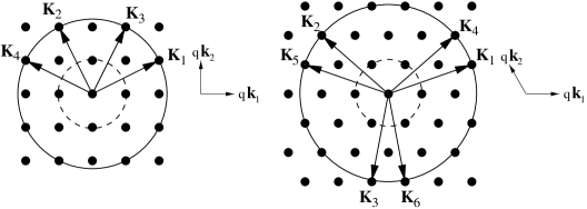
Figure 1: Square and hexagonal lattices in Fourier-space plotted together with two examples of critical circles of radius $q_{c}$. The dashed circles corresponds to $q_{c}=q$ in (11) and (12), i.e. $(m,n)=(1,0)$; the solid circle corresponds to $(m,n)=(2,1)$ on the square lattice and $(m,n)=(3,1)$ on the hexagonal lattice. Note that the solid circle has twice as many critical modes as the dashed circle.

In this paper we consider a discrete set of values of $q$, parameterized by an integer pair $(m,n)$, which admit wave vectors in (10) with length $q_{c}$, i.e., for which $|q(m\widehat{\bf k}_{1}+n\widehat{\bf k}_{2})|=q_{c}$. Specifically, on the square lattice the values of $q$ are related to $(m,n)$ by

$$q^{2}=q_{c}^{2}/(m^{2}+n^{2}),$$ (11)

and on the hexagonal lattice by

$$q^{2}=q_{c}^{2}/(m^{2}+n^{2}-mn)\ .$$ (12)

In a neighborhood of the bifurcation point, $(a,b,c,d,K)=(a_{c},b_{c},c_{c},d_{c},K_{c})$, we apply our analysis separately to the cases where there are eight critical Fourier modes on the square lattice and twelve on the hexagonal lattice (see Figure 1). Specifically, on the square lattice, we investigate primary steady solution branches of the form

$$z_{1}e^{iq{\bf K}_{1}\cdot{\bf r}}+z_{2}e^{iq{\bf K}_{2}\cdot{\bf r}}+z_{3}e^{iq{\bf K}_{3}\cdot{\bf r}}+z_{4}e^{iq{\bf K}_{4}\cdot{\bf r}}+{\rm c.c.}+\cdots$$ (13)

where $z_{1},\ldots,z_{4}$ are the complex-valued amplitudes of the critical modes, $\cdots$ represents the linearly-damped Fourier modes that are slaved to the critical modes, and ${\bf K}_{1}=(m,n)$, ${\bf K}_{2}=(-n,m)$, ${\bf K}_{3}=(n,m)$, and ${\bf K}_{4}=(-m,n)$. Note that, while ${\bf K}_{1}\cdot{\bf K}_{2}={\bf K}_{3}\cdot{\bf K}_{4}=0$, the angle between ${\bf K}_{1}$ and ${\bf K}_{3}$ depends on the integer pair $(m,n)$. Similarly, on the hexagonal lattice,

$$\sum_{n=1}^{6}z_{n}e^{iq{\bf K}_{n}\cdot{\bf r}}+{\rm c.c.}+\cdots$$ (14)

where ${\bf K}_{1}=m(1,0)+n(-1/2,\sqrt{3}/2)$ and ${\bf K}_{4}=m(1,0)+(m-n)(-1/2,\sqrt{3}/2)$. ${\bf K}_{2}$ and ${\bf K}_{3}$ are obtained by rotating ${\bf K}_{1}$ by $\pm 2\pi/3$, and ${\bf K}_{5}$ and ${\bf K}_{6}$ are obtained by rotating ${\bf K}_{4}$ by $\pm 2\pi/3$ (see Figure 1). Note that the angle between ${\bf K}_{1}$ and ${\bf K}_{4}$ again depends on $(m,n)$.

Dionne and Golubitsky [8] used the equivariant branching lemma [7] to prove that for the square lattice cases (13), the following types of steady solutions arise in pitchfork bifurcations from the spatially-uniform state:

• Stripes: ${\bf z}\equiv(z_{1},z_{2},z_{3},z_{4})=(x,0,0,0)$

• Simple squares: ${\bf z}=(x,x,0,0)$

• Rhombs: ${\bf z}=(x,0,x,0)$ and $(x,0,0,x)$

• Super squares: ${\bf z}=(x,x,x,x)$

• Anti-squares: ${\bf z}=(x,x,-x,-x)$,

where in each case $x$ is a real amplitude. (Examples of super and anti-squares are given in Section 5.2, Figure 9). While the striped and simple square patterns are essentially the same for each $m$ and $n$, the solutions in the form of rhombs, super squares and anti-squares differ for each co-prime $m$ and $n$ since the angle between ${\bf K}_{1}$ and ${\bf K}_{3}$ (and ${\bf K}_{1}$ and ${\bf K}_{4}$) depends on $m$ and $n$. The general form of the amplitude equations describing the branching and relative stability of the square lattice patterns is derived in [9]. To cubic order the bifurcation equations take the simple form

$$\dot{z}_{1}=\mu z_{1}+z_{1}(a_{1}|z_{1}|^{2}+a_{2}|z_{2}|^{2}+a_{3}|z_{3}|^{2}+a_{4}|z_{4}|^{2})+\cdots$$ (15)

with similar expressions for $\dot{z}_{2}$, $\dot{z}_{3}$, $\dot{z}_{4}$ and their conjugates. Here $\mu$ is the bifurcation parameter and $a_{1},\ldots,a_{4}$ are real. Linearizing (15) about a particular solution generates a set of eigenvalues which determines the stability of that solution with respect to perturbations on the lattice. The signs of these eigenvalues are given in Table 1 in terms of $a_{1},\ldots,a_{4}$; a positive eigenvalue indicates instability. Note that higher order terms are necessary to determine the relative stability of the super square and anti-square patterns [9]. In the next section we compute the coefficients $a_{1},\ldots,a_{4}$ needed to evaluate the signs of the eigenvalues in terms of the angle between ${\bf K}_{1}$ and ${\bf K}_{3}$ and in terms of parameters in the general reaction diffusion system (2.1).

Table 1: Signs of eigenvalues for primary bifurcation branches on the square lattice; $a_{1},\ldots,a_{4}$ are coefficients in the bifurcation equation (15). See [9] for more details.

Planform	Signs of non-zero eigenvalues
Stripes	${\rm sgn}(a_{1}),\quad{\rm sgn}(a_{2}-a_{1}),\par\quad{\rm sgn}(a_{3}-a_{1}),\quad{\rm sgn}(a_{4}-a_{1})$
${\bf z}=(x,0,0,0)$
Simple Squares	${\rm sgn}(a_{1}+a_{2}),\quad{\rm sgn}(a_{1}-a_{2}),\quad{\rm sgn}(a_{3}+a_{4}-a_{1}-a_{2})$
${\bf z}=(x,x,0,0)$
Rhombs	${\rm sgn}(a_{1}+a_{3}),\quad{\rm sgn}(a_{1}-a_{3}),\quad{\rm sgn}(a_{2}+a_{4}-a_{1}-a_{3})$
${\bf z}=(x,0,x,0)$
Rhombs	${\rm sgn}(a_{1}+a_{4}),\quad{\rm sgn}(a_{1}-a_{4}),\quad{\rm sgn}(a_{2}+a_{3}-a_{1}-a_{4})$
${\bf z}=(x,0,0,x)$
Super Squares	${\rm sgn}(a_{1}+a_{2}+a_{3}+a_{4}),\quad{\rm sgn}(a_{1}+a_{2}-a_{3}-a_{4})$
${\bf z}=(x,x,x,x)$	${\rm sgn}(a_{1}-a_{2}+a_{3}-a_{4}),\quad{\rm sgn}(a_{1}-a_{2}-a_{3}+a_{4})$
	${\rm sgn}(\zeta_{0})$, where $\zeta_{0}={\rm O}\bigl{(}x^{2(m+n-1)}\bigr{)}$
Anti–Squares	same as super squares, except $\zeta_{0}\to-\zeta_{0}$
${\bf z}=(x,x,-x,-x)$

Dionne and Golubitsky [8] also considered the hexagonal lattice problem and used group theoretic methods to determine that there are primary branches of the form

• Stripes: ${\bf z}\equiv(z_{1},z_{2},z_{3},z_{4},z_{5},z_{6})=(x,0,0,0,0,0)$

• Simple hexagons: ${\bf z}=(x,x,x,0,0,0)$

• Rhombs: ${\bf z}=(x,0,0,x,0,0)$, $(x,0,0,0,x,0)$, and $(x,0,0,0,0,x)$

• Super hexagons: ${\bf z}=(x,x,x,x,x,x)\ .$

Recently, Silber and Proctor [11] showed that there is an additional primary solution branch that has triangular symmetry:

• Super triangles: ${\bf z}=(z,z,z,z,z,z)\ \quad z\in{\bf C},$

where, near the bifurcation point, the argument of the complex amplitude $z$ is $\sim{\pi\over 3},{2\pi\over 3}$. The stripes and simple hexagons are the same for each integer pair $(m,n)$, while the other solutions change with the values of $m$ and $n$. The general form of the bifurcation equations describing the evolution of the critical modes $z_{1},\ldots,z_{6}$ is derived in [9]. The cubic truncation is

$$\dot{z}_{1} = \mu z_{1}+\gamma z_{2}^{*}z_{3}^{*}+z_{1}(b_{1}|z_{1}|^{2}+b_{2}(|z_{2}|^{2}+|z_{3}|^{2})$$ (17)

$$\qquad\qquad\qquad\qquad+b_{4}|z_{4}|^{2}+b_{5}|z_{5}|^{2}+b_{6}|z_{6}|^{2})+\cdots$$

with similar expressions for $\dot{z}_{2},\ldots,\dot{z}_{6}$. While the stripes and rhombs solutions arise from the uniform state in a pitchfork bifurcation, all other solutions bifurcate transcritically. The relative stability of the primary patterns are summarized from [9] in Table 2. Note that unless the quadratic coefficient $\gamma$ is zero, all branches bifurcate unstably. Thus we will consider a degenerate bifurcation problem for which $\gamma\approx 0$. Also note that, as in the case of super squares and anti-squares, the relative stability of the super hexagons and super triangles is determined by terms higher than cubic in (17) [11].

Table 2: Branching equations and signs of eigenvalues for primary bifurcation branches on the hexagonal lattice; $\gamma,b_{1},\dots,b_{6}$ are coefficients in the bifurcation equation (17). See [9, 10] for more details.

Planform and branching equation	Signs of non-zero eigenvalues
Stripes	${\rm sgn}(b_{1})$,
${\bf z}=(x,0,0,0,0,0)$	${\rm sgn}(\gamma x+(b_{2}-b_{1})x^{2}),\quad{\rm sgn}(-\gamma x+(b_{2}-b_{1})x^{2})$,
$0=\mu x+b_{1}x^{3}+{\rm O}(x^{5})$	${\rm sgn}(b_{4}-b_{1}),\quad{\rm sgn}(b_{5}-b_{1}),\quad{\rm sgn}(b_{6}-b_{1})$
Simple Hexagons	${\rm sgn}(\gamma x+2(b_{1}+2b_{2})x^{2}),\quad{\rm sgn}(-\gamma x+(b_{1}-b_{2})x^{2}$)
${\bf z}=(x,x,x,0,0,0)$	${\rm sgn}(-\gamma x+(b_{4}+b_{5}+b_{6}-b_{1}-2b_{2})x^{2})$
$0=\mu x+\gamma x^{2}+(b_{1}+2b_{2})x^{3}+{\rm O}(x^{4})$	${\rm sgn}(-\gamma x+{\rm O}(x^{3}))$
Rhombs	${\rm sgn}(b_{1}+b_{4}),\quad{\rm sgn}(b_{1}-b_{4}),\quad{\rm sgn}(\zeta_{1}),\quad{\rm sgn}(\zeta_{2}),$
${\bf z}=(x,0,0,x,0,0)$	where $\zeta_{1}+\zeta_{2}=(-2b_{1}-2b_{4}+2b_{2}+b_{5}+b_{6})x^{2}$,
$0=\mu x+(b_{1}+b_{4})x^{3}+{\rm O}(x^{5})$	$\zeta_{1}\zeta_{2}=-\gamma^{2}x^{2}+(b_{1}+b_{4}-b_{2}-b_{5})(b_{1}+b_{4}-b_{2}-b_{6})x^{4}$
Rhombs	${\rm sgn}(b_{1}+b_{5}),\quad{\rm sgn}(b_{1}-b_{5}),\quad{\rm sgn}(\zeta_{1}),\quad{\rm sgn}(\zeta_{2}),$
${\bf z}=(x,0,0,0,x,0)$	where $\zeta_{1}+\zeta_{2}=(-2b_{1}-2b_{5}+2b_{2}+b_{4}+b_{6})x^{2}$,
$0=\mu x+(b_{1}+b_{5})x^{3}+{\rm O}(x^{5})$	$\zeta_{1}\zeta_{2}=-\gamma^{2}x^{2}+(b_{1}+b_{5}-b_{2}-b_{4})(b_{1}+b_{5}-b_{2}-b_{6})x^{4}$
Rhombs	${\rm sgn}(b_{1}+b_{6}),\quad{\rm sgn}(b_{1}-b_{6}),\quad{\rm sgn}(\zeta_{1}),\quad{\rm sgn}(\zeta_{2}),$
${\bf z}=(x,0,0,0,0,x)$	where $\zeta_{1}+\zeta_{2}=(-2b_{1}-2b_{6}+2b_{2}+b_{4}+b_{5})x^{2}$
$0=\mu x+(b_{1}+b_{6})x^{3}+{\rm O}(x^{5})$	$\zeta_{1}\zeta_{2}=-\gamma^{2}x^{2}+(b_{1}+b_{6}-b_{2}-b_{4})(b_{1}+b_{6}-b_{2}-b_{5})x^{4}$
	${\rm sgn}(\gamma x+2(b_{1}+2b_{2}+b_{4}+b_{5}+b_{6})x^{2})$
Super Hexagons	${\rm sgn}(\gamma x+2(b_{1}+2b_{2}-b_{4}-b_{5}-b_{6})x^{2})$
${\bf z}=(x,x,x,x,x,x)$	${\rm sgn}(-\gamma x+{\rm O}(x^{3})),\quad{\rm sgn}(\zeta_{1}),\quad{\rm sgn}(\zeta_{2})$,
$0=\mu x+\gamma x^{2}+(b_{1}+2b_{2})x^{3}\quad$	where $\zeta_{1}+\zeta_{2}=-4\gamma x+4(b_{1}-b_{2})x^{2}$
$\qquad+(b_{4}+b_{5}+b_{6})x^{3}+{\rm O}(x^{4})$	$\zeta_{1}\zeta_{2}=4(\gamma x-(b_{1}-b_{2})x^{2})^{2}\qquad\qquad\qquad\quad$
	$\qquad\qquad\qquad-2((b_{4}-b_{5})^{2}+(b_{4}-b_{6})^{2}+(b_{5}-b_{6})^{2}))x^{4}$
	${\rm sgn}(\zeta_{0})$, where $\zeta_{0}={\rm O}(x^{2(m-1)})$
Super Triangles
${\bf z}=(z,z,z,z,z,z),$	Same as super hexagons
$\quad z=xe^{i\psi},\psi\neq 0,\pi,\ldots$	except $\zeta_{0}\to-\zeta_{0}$
$0=\mu z+\gamma\bar{z}^{2}+(b_{1}+2b_{2})|z|^{2}z\quad$
$\qquad+(b_{4}+b_{5}+b_{6})|z|^{2}z+{\rm O}(x^{4})$

3 Reduction to Bifurcation Equations

Although symmetry determines the form of the bifurcation equations, the particular system determines $a_{n}$ (and $b_{n}$) in equations (15) (and (17)). Each coefficient $a_{n}$ is associated with a particular amplitude $z_{n}$ in (15), and each of these amplitudes is in turn associated with a Fourier wave vector ${\bf K}_{n}$. In this section we use perturbation theory to derive the coefficients $a_{n}$, $\gamma$, and $b_{n}$ from the full system (2.1).

The coefficients $a_{1},\ldots,a_{4}$ and $b_{1}(=a_{1}),b_{4},b_{5},b_{6}$ may all be calculated by considering a single bifurcation problem involving just two critical Fourier modes; the remaining coefficients $\gamma$ and $b_{2}$ are calculated by considering a bifurcation to hexagons. To understand the need for only two modes in the computation of $a_{1},\ldots,a_{4},b_{4},b_{5},b_{6}$ consider, for example, the square lattice, where the ${\bf K}_{2},{\bf K}_{3},$ and ${\bf K}_{4}$ vectors are all related to the ${\bf K}_{1}$ vector by an angle $\theta$. Let $\theta_{j}$ denote the angle between ${\bf K}_{1}$ and ${\bf K}_{j}$; then $\theta_{2}=\pi/2$ and $\theta_{4}=\pi/2+\theta_{3}$ where $\theta_{3}$ is related to the integer pair $(m,n)$ by

$$\cos\theta_{3}={2mn\over m^{2}+n^{2}}$$ (18)

(see Figure 1). The coefficients $a_{j}$ are a function of the angle $\theta_{j}$:

$$a_{j}=h(\theta_{n}),\quad j=2,3,4.$$

Similarly, on the hexagonal lattice,

$$b_{j}=h(\theta_{j}),\quad j=4,5,6$$

where $\theta_{5}=\theta_{4}+2\pi/3$ and $\theta_{6}=\theta_{4}+4\pi/3$, with $\theta_{4}$ determined by the integers $(m,n)$. From symmetry considerations we know that $h(\theta)=h(\pi-\theta)$. A calculation with two critical modes will determine $h(\theta)$, and hence determine all of the angle-dependent coefficients in the bifurcation equations.

To compute $h(\theta)$ we seek solutions which are periodic on a rhombic (or square) lattice; specifically, solutions of the form

$$w_{\rm rh}=z_{1}e^{i{\bf k}_{1}\cdot{\bf r}}+z_{\theta}e^{i{\bf k}_{\theta}\cdot{\bf r}}+{\rm c.c.},$$ (19)

where ${\bf k}_{1}=q_{c}(1,0)$, ${\bf k}_{\theta}=q_{c}(\cos\theta,\sin\theta)$, and $\theta$ is not a multiple of $\pi/3$. The amplitudes evolve in a neighborhood of the bifurcation point $\mu=0$ according to

$$\dot{z}_{1} = \mu z_{1}+z_{1}(a_{1}|z_{1}|^{2}+h(\theta)|z_{\theta}|^{2})$$

$$\dot{z}_{\theta} = \mu z_{\theta}+z_{\theta}(a_{1}|z_{\theta}|^{2}+h(\theta)|z_{1}|^{2}).$$ (20)

Stripes are solutions satisfying $z_{\theta}=0$; rhombs correspond to $z_{1}=z_{\theta}$; squares correspond to $z_{1}=z_{\pi/2}$. Comparison of (20) with (15) restricted to the subspace ${\bf z}=(z_{1},0,z_{\theta},0)$ confirms the relationship $a_{3}=h(\theta_{3})$, etc.

To compute $\gamma$ and $b_{2}$ in equation (17) we consider a three-mode solution

$$w_{\rm hex}=z_{1}e^{i{\bf k}_{1}\cdot{\bf r}}+z_{2}e^{i{\bf k}_{2}\cdot{\bf r}}+z_{3}e^{i{\bf k}_{3}\cdot{\bf r}}+{\rm c.c.},$$ (21)

where ${\bf k}_{1}=q_{c}(1,0)$, ${\bf k}_{2}=q_{c}(-1/2,\sqrt{3}/2)$, and ${\bf k}_{3}=q_{c}(-1/2,-\sqrt{3}/2)$. The amplitudes evolve according to equations of the form

$$\dot{z}_{1}=\mu z_{1}+\gamma z_{2}^{*}z_{3}^{*}+z_{1}(b_{1}|z_{1}|^{2}+b_{2}(|z_{2}|^{2}+|z_{3}|^{2}))$$ (22)

with similar equations for $\dot{z}_{2}$ and $\dot{z}_{3}$.

To compute the bifurcation equations (20) and (22) from equation (2.1) we first Taylor-expand $f(u,v)$ and $g(u,v)$ through cubic order in $u$ and $v$:

$$f(u,v) = au+bv+F_{2}(u,v)+F_{3}(u,v)+\cdots$$

$$g(u,v) = cu+dv+G_{2}(u,v)+G_{3}(u,v)+\cdots.$$

Here $F_{2}(u,v)$, $G_{2}(u,v)$, $F_{3}(u,v)$, and $G_{3}(u,v)$ denote the quadratic and cubic nonlinear terms:

$$\left(\matrix{F_{2}(u,v)\cr G_{2}(u,v)\cr}\right) \equiv \left(\matrix{f_{uu}u^{2}/2+f_{uv}uv+f_{vv}v^{2}/2\cr g_{uu}u^{2}/2+g_{uv}uv+g_{vv}v^{2}/2\cr}\right),$$

$$\vskip 6.0pt plus 2.0pt minus 2.0pt\left(\matrix{F_{3}(u,v)\cr G_{3}(u,v)\cr}\right) \equiv \left(\matrix{f_{uuu}u^{3}/6+f_{uuv}u^{2}v/2+f_{uvv}uv^{2}/2+f_{vvv}v^{3}/6\cr g_{uuu}u^{3}/6+g_{uuv}u^{2}v/2+g_{uvv}uv^{2}/2+g_{vvv}v^{3}/6\cr}\right),$$

where the subscripts on $f$ and $g$ denote partial derivatives evaluated at $u=v=0$.

We use perturbation theory to compute the small amplitude, slow evolution on the center manifold. Let

$$t_{1}=\epsilon t,\quad t_{2}=\epsilon^{2}t,$$

$$\left(\matrix{u\cr v\cr}\right)=\epsilon\left(\matrix{u_{1}\cr v_{1}\cr}\right)w_{1}({\bf r},t_{1},t_{2})+\epsilon^{2}{\bf W}_{2}+\epsilon^{3}{\bf W}_{3}+O(\epsilon^{4}),$$ (23)

where $w_{1}$ takes the form of either (19) or (21) for the respective rhombic or hexagonal calculations, and ${\bf W}_{2}$ and ${\bf W}_{3}$ represent higher order terms to be determined. The vector $(u_{1},v_{1})^{T}$ is a null-vector of $L(q_{c})$, at the bifurcation point; see equation (3). We further assume that the linear parameters $a,b,c,d,K$ are within $O(\epsilon^{2})$ of the critical bifurcation values, e.g. $a=a_{c}+\epsilon^{2}\lambda_{a}$, etc. where $a_{c},b_{c},c_{c},d_{c},K_{c}$ satisfy (8) and determine $q_{c}$ via substitution into (7). With these assumptions, equation (2.1) may be written as

$$\epsilon^{2}{\partial\over\partial t_{2}}\left(\matrix{u\cr v\cr}\right)+\epsilon{\partial\over\partial t_{1}}\left(\matrix{u\cr v\cr}\right)+L_{0}\left(\matrix{u\cr v\cr}\right)=\epsilon^{2}L_{2}\left(\matrix{u\cr v\cr}\right)+\left(\matrix{F_{2}(u,v)\cr G_{2}(u,v)\cr}\right)+\left(\matrix{F_{3}(u,v)\cr G_{3}(u,v)\cr}\right)$$ (24)

plus higher order terms, where

$$L_{0}\equiv\left(\matrix{-\nabla^{2}-a_{c}&-b_{c}\cr-c_{c}&-K_{c}\nabla^{2}-d_{c}\cr}\right)$$

and

$$L_{2}\equiv\left(\matrix{\lambda_{a}&\lambda_{b}\cr\lambda_{c}&\lambda_{d}+\lambda_{K}\nabla^{2}\cr}\right).$$

3.1 Rhombic Lattice Computation

For the rhombic case, the equation for ${\bf W}_{2}$ is given at $O(\epsilon^{2})$ as

$$\left(\matrix{u_{1}\cr v_{1}\cr}\right){\partial\over\partial t_{1}}w_{\rm rh}+L_{0}{\bf W}_{2}=\left(\matrix{F_{2}(u_{1},v_{1})\cr G_{2}(u_{1},v_{1})\cr}\right)w_{\rm rh}^{2},$$ (25)

where $w_{\rm rh}$ is given by (19). Through the term $w_{\rm rh}^{2}$ the quadratic nonlinearities generate four terms with distinct wave numbers:

$$w_{2} = z_{1}^{2}e^{i2{\bf k}_{1}\cdot{\bf r}}+z_{\theta}^{2}e^{i2{\bf k}_{\theta}\cdot{\bf r}}+{\rm c.c.},\quad\nabla^{2}w_{2}=-4q_{c}^{2}w_{2},$$

$$w_{3} = z_{1}z_{\theta}e^{i({\bf k}_{1}+{\bf k}_{\theta})\cdot{\bf r}}+{\rm c.c.},\quad\nabla^{2}w_{3}=-2q_{c}^{2}(1+\cos\theta)w_{3},$$

$$w_{4} = z_{1}z_{\theta}^{*}e^{i({\bf k}_{1}-{\bf k}_{\theta})\cdot{\bf r}}+{\rm c.c.},\quad\nabla^{2}w_{4}=-2q_{c}^{2}(1-\cos\theta)w_{4},$$

$$w_{5} = |z_{1}|^{2}+|z_{\theta}|^{2},\quad\nabla^{2}w_{5}=0.$$

There are no terms on the right hand side of (25) with wave number $q_{c}$, so the solvability condition is

$${\partial\over\partial t_{1}}w_{\rm rh}=0.$$

Since there is no dependence on the $t_{1}$-time scale it will be omitted from the remaining analysis. Solving equation (25) determines

$${\bf W}_{2}\equiv\left(\matrix{U_{2}\cr V_{2}\cr}\right)=\sum_{n=2}^{5}\left(\matrix{u_{n}\cr v_{n}\cr}\right)w_{n},$$ (26)

where $u_{n}$ and $v_{n}$ ($n=2,\ldots,5$) are constant and satisfy

$$L_{0}\left(\matrix{u_{n}\cr v_{n}\cr}\right)w_{n}=\left(\matrix{F_{2}(u_{1},v_{1})\cr G_{2}(u_{1},v_{1})}\right)c_{n}w_{n},$$ (27)

where $c_{2}=1$ and $c_{3}=c_{4}=c_{5}=2$. Explicit expressions for $u_{n}$ and $v_{n}$ are given in the Appendix.

The equation at $O(\epsilon^{3})$ is

$$\left(\matrix{u_{1}\cr v_{1}\cr}\right){\partial\over\partial t_{2}}w_{\rm rh}+L_{0}{\bf W}_{3} = L_{2}\left(\matrix{u_{1}\cr v_{1}\cr}\right)w_{\rm rh}+\left(\matrix{{\partial F_{2}(u_{1},v_{1})\over\partial u_{1}}\cr{\partial G_{2}(u_{1},v_{1})\over\partial u_{1}}\cr}\right)U_{2}w_{\rm rh}$$ (28)

$$+\left(\matrix{{\partial F_{2}(u_{1},v_{1})\over\partial v_{1}}\cr{\partial G_{2}(u_{1},v_{1})\over\partial v_{1}}\cr}\right)V_{2}w_{\rm rh}$$

$$+\left(\matrix{F_{3}(u_{1},v_{1})\cr G_{3}(u_{1},v_{1})\cr}\right)w_{\rm rh}^{3},$$

where $(U_{2},V_{2})$ are given by (26). There are now terms on the right hand side of the equation with spatial dependence $e^{i{\bf k}_{1}\cdot{\bf r}}$ and $e^{i{\bf k}_{\theta}\cdot{\bf r}}$; the operator $L_{0}$ is not invertible for terms with this Fourier dependence. To ensure that these terms will lie in the range of $L_{0}$ we apply the Fredholm alternative theorem to obtain the solvability condition. In this computation we use the fact that the nullspace of the adjoint linear operator $L_{0}^{\dagger}$ is spanned by

$$(\tilde{u},\tilde{v})e^{i{\bf k}_{1}\cdot{\bf r}},\quad(\tilde{u},\tilde{v})e^{i{\bf k}_{\theta}\cdot{\bf r}},$$

where

$$\left(\tilde{u},\tilde{v}\right)=\left(c,-a_{c}+q_{c}^{2}\right).$$ (29)

The inner product of equation (28) with these left null-vectors yields the solvability condition, which takes the expected form of the bifurcation equations (20). After rescaling time to absorb the factor $u_{1}\tilde{u}+v_{1}\tilde{v}$, which is always positive, we obtain the rhombic bifurcation equation coefficients

$$a_{1}=(u_{2}+u_{5})\eta_{1}+(v_{2}+v_{5})\eta_{2}+3\beta$$ (30)

and

$$h(\theta)=(u_{3}+u_{4}+u_{5})\eta_{1}+(v_{3}+v_{4}+v_{5})\eta_{2}+6\beta,$$ (31)

where

$$\eta_{1} \equiv \tilde{u}{\partial F_{2}(u_{1},v_{1})\over\partial u_{1}}+\tilde{v}{\partial G_{2}(u_{1},v_{1})\over\partial u_{1}},$$

$$\eta_{2} \equiv \tilde{u}{\partial F_{2}(u_{1},v_{1})\over\partial v_{1}}+\tilde{v}{\partial G_{2}(u_{1},v_{1})\over\partial v_{1}},$$ (32)

$$\beta \equiv \tilde{u}F_{3}(u_{1},v_{1})+\tilde{v}G_{3}(u_{1},v_{1}).$$

The expressions for $u_{n}$ and $v_{n}$, $n=2,\ldots,5$, are given in the Appendix.

3.2 Hexagonal Lattice Computation

The hexagonal calculation proceeds in a fashion similar to the rhombic case, but requires some additional work due to the presence of resonant terms with wave number $q_{c}$ which are generated by the quadratic nonlinearities.

To simplify the presentation we let $z_{1}=z_{2}=z_{3}=z_{h}$ in (21). Since the form of the amplitude equation is known from equation (17), and $b_{1}(=a_{1})$ is known from the rhombic lattice calculation, the remaining coefficients $\gamma$ and $b_{2}$ may be extracted from the quadratic and cubic coefficient expressions, respectively.

At $O(\epsilon^{2})$ the equation to be solved is

$$\left(\matrix{u_{1}\cr v_{1}\cr}\right){\partial\over\partial t_{1}}w_{\rm hex}+L_{0}{\bf W}_{2} = \left(\matrix{F_{2}(u_{1},v_{1})\cr G_{2}(u_{1},v_{1})\cr}\right)w_{\rm hex}^{2}$$ (33)

where $w_{\rm hex}$ is given by (21). The term $w_{\rm hex}^{2}$ generates four terms with distinct wave numbers:

$$w_{2} = z_{h}^{2}(e^{i2{\bf k}_{1}\cdot{\bf r}}+e^{i2{\bf k}_{2}\cdot{\bf r}}+e^{i2{\bf k}_{3}\cdot{\bf r}})+{\rm c.c.},\quad\nabla^{2}w_{2}=-4q_{c}^{2}w_{2},$$

$$w_{5} = |z_{h}|^{2},\quad\nabla^{2}w_{5}=0,$$

$$w_{6} = |z_{h}|^{2}(e^{i({\bf k}_{1}-{\bf k}_{2})\cdot{\bf r}}+e^{i({\bf k}_{2}-{\bf k}_{3})\cdot r}+e^{i({\bf k}_{3}-{\bf k}_{1})\cdot{\bf r}})+{\rm c.c.},\quad\nabla^{2}w_{6}=-3q_{c}^{2}w_{6},$$

$$w_{7} = {z_{h}^{*}}^{2}(e^{i{\bf k}_{1}\cdot{\bf r}}+e^{i{\bf k}_{2}\cdot{\bf r}}+e^{i{\bf k}_{3}\cdot{\bf r}})+{\rm c.c.},\quad\nabla^{2}w_{7}=-q_{c}^{2}w_{7}.$$

From $w_{7}$ we see that there are now terms on the right hand side of (33) with wave number $q_{c}$, for which $L_{0}$ is not invertible. Unlike in the rhombic case the $t_{1}$ time scale is necessary here, reflecting that the small-amplitude dynamics are dominated by the quadratic nonlinearities. As in the rhombic calculation the Fredholm alternative theorem is applied, giving the solvability condition

$$(u_{1}\tilde{u}+v_{1}\tilde{v}){\partial\over\partial t_{1}}z_{h} = \gamma{z_{h}^{*}}^{2},\qquad\gamma=2(\tilde{u}F_{2}(u_{1},v_{1})+\tilde{v}G_{2}(u_{1},v_{1})).$$ (34)

The factor $(u_{1}\tilde{u}+v_{1}\tilde{v})$ is positive (from conditions (8) and (9)) and will later be absorbed by a rescaling of time. Note that if $\gamma$ is $O(\epsilon)$ then the $t_{1}$-time scale is unnecessary. This is the situation of interest here, since we know from Table 2 that when $\gamma$ is $O(1)$ there are no stable small-amplitude steady states. However, in the following computation we must retain both time scales to compute the general form of the cubic coefficient $b_{2}$. In our subsequent analysis we will focus on the degenerate problem $\gamma=0$.

Continuing as in the rhombic case, the solution of (33) is

$${\bf W}_{2}\equiv\left(\matrix{U_{2}\cr V_{2}}\right)=\sum_{n=2,5,6,7}\left(\matrix{u_{n}\cr v_{n}\cr}\right)w_{n},$$

where $u_{2}$, $v_{2}$, $u_{5}$, and $v_{5}$ are known from the rhombic lattice computation, and $u_{6}$ and $v_{6}$ are computed in a similar fashion. Equations (33) and (34) lead to the following solvable equation for $(u_{7},v_{7})$:

$$L_{0}\left(\matrix{u_{7}\cr v_{7}\cr}\right)w_{7}=-{\gamma\over u_{1}\tilde{u}+v_{1}\tilde{v}}\left(\matrix{u_{1}\cr v_{1}\cr}\right)w_{7}+2\left(\matrix{F_{2}(u_{1},v_{1})\cr G_{2}(u_{1},v_{1})\cr}\right)w_{7}.$$

We choose the particular solution of this singular problem to be

$$u_{7}=0,\quad v_{7}=-{1\over b_{c}}\left(-{\gamma u_{1}\over u_{1}\tilde{u}+v_{1}\tilde{v}}+2F_{2}(u_{1},v_{1})\right).$$

At $O(\epsilon^{3})$ the equation is

$$\left(\matrix{u_{1}\cr v_{1}\cr}\right){\partial\over\partial t_{2}}w_{\rm hex}+{\partial\over\partial t_{1}}{\bf W}_{2}+L_{0}{\bf W}_{3} = L_{2}\left(\matrix{u_{1}\cr v_{1}\cr}\right)w_{\rm hex}$$ (37)

$$+\left(\matrix{{\partial F_{2}(u_{1},v_{1})\over\partial u_{1}}\cr{\partial G_{2}(u_{1},v_{1})\over\partial u_{1}}\cr}\right)U_{2}w_{\rm hex}$$

$$+\left(\matrix{{\partial F_{2}(u_{1},v_{1})\over\partial v_{1}}\cr{\partial G_{2}(u_{1},v_{1})\over\partial v_{1}}\cr}\right)V_{2}w_{\rm hex}$$

$$+\left(\matrix{F_{3}(u_{1},v_{1})\cr G_{3}(u_{1},v_{1})\cr}\right)w_{\rm hex}^{3}.$$

Again the Fredholm alternative theorem must be applied, giving a solvability condition of the form

$$(u_{1}\tilde{u}+v_{1}\tilde{v}){\partial\over\partial t_{2}}z_{h}=\lambda z_{h}+(b_{1}+2b_{2})|z_{h}|^{2}z_{h}.$$

By letting $z(t)=\epsilon z_{h}(t_{1},t_{2})$, $\mu=\epsilon^{2}\lambda$, and rescaling time to absorb the factor $u_{1}\tilde{u}+v_{1}\tilde{v}$ on the left hand side, we obtain the reconstituted bifurcation equation

$$\dot{z}=\mu z+\gamma{z^{*}}^{2}+(b_{1}+2b_{2})|z|^{2}z.$$

The coefficients $\mu$, $\gamma$, $b_{1}$, and $b_{2}$ are given in the Appendix.

4 Parameter Collapse

Naively one might expect that the cubic coefficients $a_{n}$ and $b_{n}$ in the bifurcation equations may be adjusted to take on any desired value, by varying the many nonlinear coefficients in the Taylor expansions of $f(u,v)$ and $g(u,v)$. However, the expressions for $a_{n}$ and $b_{n}$, given in Appendix A, clearly show that all eight cubic coefficients contained within $F_{3}(u_{1},v_{1})$ and $G_{3}(u_{1},v_{1})$ collapse into the single expression $\beta\equiv\tilde{u}F_{3}(u_{1},v_{1})+\tilde{v}G_{3}(u_{1},v_{1})$. Similarly, the six quadratic coefficients in $F_{2}(u,v)$ and $G_{2}(u,v)$ are contained in the coefficient expressions solely in the four terms $F_{2}(u_{1},v_{1})$, $G_{2}(u_{1},v_{1})$, $\eta_{1}$ and $\eta_{2}$, given by (32). Moreover, these last four quantities satisfy the relation

$$u_{1}\eta_{1}+v_{1}\eta_{2}=2\tilde{u}F_{2}(u_{1},v_{1})+2\tilde{v}G_{2}(u_{1},v_{1}).$$ (38)

Therefore the six quadratic coefficients collapse into three independent parameters. In summary, the fourteen nonlinear coefficients in the Taylor expansions of $f(u,v)$ and $g(u,v)$ enter our analysis in just four independent combinations.

4.1 Hexagonal degeneracy

The parameter collapse is even more dramatic at the degeneracy $\gamma=0$ in the hexagonal bifurcation problem (17). An additional striking phenomena occurs at this point, which results in all $\theta$-dependence of the coefficients dropping out, thereby severely restricting the types of patterns which may bifurcate stably. Below we show that the bifurcation equations depend on just two quantities determined from the reaction kinetics of (2.1). Thus, we may simply and completely characterize the possible bifurcation scenarios for all reaction-diffusion systems of the form (2.1) restricted to the hexagonal bifurcation problem at the degeneracy.

The degeneracy condition is

$$\gamma\equiv\tilde{u}F_{2}(u_{1},v_{1})+\tilde{v}G_{2}(u_{1},v_{1})=0,$$ (39)

which implies

$$u_{1}\eta_{1}+v_{1}\eta_{2}=0$$ (40)

by substitution into (38). These two equations may be solved for $F_{2}$ and $\eta_{1}$ in terms of $G_{2}$ and $\eta_{2}$, and therefore these four parameters collapse into the single parameter combination $\eta_{2}G_{2}(u_{1},v_{1})$ in the coefficient expressions for $a_{n}$ and $b_{n}$.

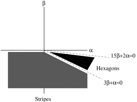
Figure 2: Stability of patterns at the hexagonal degeneracy $\gamma=0$. The details of $f(u,v)$ and $g(u,v)$ in (2.1) enter the stability analysis via two effective parameters: $\alpha$, which depends on the quadratic nonlinearities, and $\beta$, which depends on the cubic nonlinearities. Rhombs and super hexagons are always unstable, as shown in Section 4.1. All patterns bifurcate unstably for $\beta>0$ and/or $15\beta+2\alpha>0$. For the region labeled “hexagons” we have determined only that hexagons are neutrally stable, since their stability for $\gamma=0$ depends on terms higher than cubic in (17).

The bifurcation coefficients $b_{1}=a_{1}$, $h(\theta)$, and $b_{2}$ contain the terms $u_{2},v_{2},\ldots,u_{6},v_{6}$, as given in the Appendix (see also equations (30) and (31)). These terms are determined by solving equations of the form (cf. (27))

$$-L_{0}(q_{c})\left(\matrix{u_{n}\cr v_{n}\cr}\right)+q_{c}^{2}f_{n}(\theta)\left(\matrix{1&0\cr 0&K\cr}\right)\left(\matrix{u_{n}\cr v_{n}\cr}\right)=c_{n}\left(\matrix{F_{2}(u_{1},v_{1})\cr G_{2}(u_{1},v_{1})\cr}\right).$$

Here $L_{0}(q_{c})$ is the singular matrix (3) from the linear calculation, $c_{n}$ is a constant, and $f_{n}(\theta)$ is nonzero; for example, $f_{3}(\theta)=1+2\cos\theta$. Multiplying the above equation by the left null-vector $(\tilde{u},\tilde{v})$ of $L_{0}(q_{c})$ gives

$$\tilde{u}u_{n}+K\tilde{v}v_{n}=0$$

at the degeneracy. Using this relation and relation (40), we see that

$$u_{n}\eta_{1}+v_{n}\eta_{2}=v_{n}\eta_{2}\left({Kv_{1}\tilde{v}\over u_{1}\tilde{u}}+1\right).$$

From the definitions of the null-vectors $(u_{1},v_{1})$ and $(\tilde{u},\tilde{v})$ it immediately follows that

$$u_{n}\eta_{1}+v_{n}\eta_{2}=0,\quad n=2,\ldots,6.$$

These expressions may then be substituted into the bifurcation coefficient expressions from the Appendix, giving

$$b_{1}\equiv(u_{2}+u_{5})\eta_{1}+(v_{2}+v_{5})\eta_{2}+3\beta=3\beta,$$

$$h(\theta)\equiv(u_{3}+u_{4}+u_{5})\eta_{1}+(v_{3}+v_{4}+v_{5})\eta_{2}+6\beta=6\beta,$$

$$b_{2}\equiv(u_{5}+u_{7})\eta_{1}+(v_{5}+v_{6}+v_{7})\eta_{2}-2\gamma(\tilde{v}v_{6})+6\beta=v_{7}\eta_{2}+6\beta,$$

for $\gamma=0$. In short, the quadratic nonlinearities from $F_{2}(u,v)$ and $G_{2}(u,v)$ completely disappear from the bifurcation coefficients $b_{1}$ and $h(\theta)$, and appear in $b_{2}$ solely through the term

$$\alpha\equiv v_{7}\eta_{2}.$$ (41)

This further implies that all $\theta$-dependence disappears from the bifurcation equations, and that rhombs and super hexagons are always unstable at the bifurcation point, for the degenerate problem. The signs of the eigenvalues for rhombs and super hexagons are given in Table 2. The first two eigenvalues for rhombs depend on the signs of $b_{1}+b_{4}$ and $b_{1}-b_{4}$, which cannot both be negative. Hence rhombs are always unstable. The signs of the first three super hexagon eigenvalues are determined by the signs of

$$e_{1}\equiv b_{1}+2b_{2}+b_{4}+b_{5}+b_{6}=33\beta+2\alpha,$$

$$e_{2}\equiv b_{1}+2b_{2}-b_{4}-b_{5}-b_{6}=-3\beta+2\alpha,$$

$$e_{3}\equiv b_{1}-b_{2}=-3\beta-\alpha.$$

All three cannot be made negative, since $e_{1}=-(3e_{2}+8e_{3})$. Stripes and hexagons may bifurcate stably; Figure 2 gives their stability assignments in the $(\alpha,\beta)$-parameter plane. Note that, for the cubic truncation of the bifurcation problem, hexagons are only known to be neutrally stable, since the eigenvalue $-\gamma x+O(x^{3})$ in Table 2 depends on higher-order terms, which are not computed here. For the corresponding square lattice computation, stripes are stable for $\beta<0$; all other solutions are unstable for $\gamma=0$. This picture can be made even simpler for systems with $F_{2}(u,v)\propto G_{2}(u,v)$, such as the CIMA model considered in the next section. In these systems, $\gamma=0$ typically implies $F_{2}(u_{1},v_{1})=G_{2}(u_{1},v_{1})=0$, leading to $\alpha=0$ in Figure 2. Stripes are then stable provided $\beta<0$.

Figure 3: Hexagonal lattice bifurcation diagram for the reaction-diffusion system with $\gamma=0.03$, $\alpha=-2$, and $\beta=-1/3$, as described in Section 4.1. Secondary branches and unstable primary branches are not plotted. Clearly there is a range of $\mu$ for which this system is tri-stable.

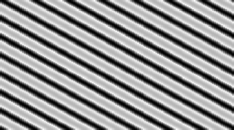
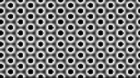
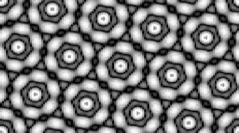
Figure 4: The steady state concentration field $u({\bf r})$ in the form of stripes, hexagons, and super hexagons, as computed numerically from the reaction-diffusion system (2.1) with reaction-kinetics given by (42). The sole difference between these numerical runs was in the initial condition. Compare with the bifurcation diagram given in Figure 3. Numerical simulations were performed with a pseudo-spectral Crank-Nicholson scheme, using second-order Adams-Bashforth on the nonlinear terms. The rectangular domain has aspect ratio $\sqrt{3}$, with a 128$\times$128 grid.

We next unfold the degenerate problem by considering $0<|\gamma|\ll 1$ in (21), keeping $b_{1}=3\beta$, $b_{2}=\alpha+6\beta$, and $b_{4}=b_{5}=b_{6}=6\beta$. There is now a small range of values $\mu\in(\mu_{1},\mu_{2})$ for which super hexagons (or triangles) are stable, provided that $\alpha<0$, $\beta\in(\alpha/3,-\alpha/21)$. For example, Figure 3 shows the unfolded bifurcation diagram for $\beta=-1/3$, $\alpha=-2$ $(0<\gamma\ll 1)$. It is straightforward to construct a system of the form (2.1) with these values. Let

$$K=4,$$

$$f(u,v)=(2+\lambda_{a})u-1.8v+0.2378u^{2}-0.0141u^{3},$$ (42)

$$g(u,v)=4.05u-2.8v-0.04u^{2}+uv.$$

This system gives $\gamma\approx 0.03$, $\alpha\approx-2$, $\beta\approx-1/3$, and according to the unfolding calculation gives stable super hexagons (or triangles) in the range $3.07\times 10^{-5}<\lambda_{a}<1.38\times 10^{-4}$. A value of $\lambda_{a}=7.6\times 10^{-5}$ corresponds to $\mu=5.54\times 10^{-4}$ in Figure 3, at which point rolls, hexagons, and super hexagons are all stable according to our analysis. Figure 4 shows a numerical integration of this system with $\lambda_{a}=7.6\times 10^{-5}$, using a pseudo-spectral Crank-Nicholson scheme on a $128\times 128$ rectangular grid of aspect ratio $\sqrt{3}$. All three pictures are at the same parameter values, and differ solely in the initial condition. The amplitude of the fundamental mode in each case is within two percent of the steady-state values predicted by the amplitude equations.

5 Application to Model Equations

5.1 Lengyel-Epstein model

The results of the previous sections will now be applied to a reaction-diffusion system proposed by Lengyel and Epstein [6] as a reduced model for the CIMA reaction:

$$\begin{array}[]{rcl}A_{t}&=&\hat{a}-A-{4AB\over 1+A^{2}}+\nabla^{2}A\cr B_{t}&=&\delta\hat{b}\left(A-{AB\over 1+A^{2}}+{\hat{c}\over\hat{b}}\nabla^{2}B\right).\end{array}$$ (45)

Note that the nonlinear terms differ solely by a multiplicative constant, which will further simplify the hexagonal lattice computations.

Our analysis assumes a steady-state solution of $u=v=0$. Thus we let

$$A=x_{0}+(1+x_{0}^{2})u,\quad B=(1+x_{0}^{2})(1+v)$$

where

$$x_{0}\equiv{\hat{a}\over 5}>0.$$

After expanding the nonlinearities to cubic order the equation may be written as

$$\begin{array}[]{rcl}u_{t}&=&\nabla^{2}u+au+bv+F_{2}(u,v)+F_{3}(u,v)\cr v_{t}&=&\delta\hat{b}[K\nabla^{2}v+cu+dv+G_{2}(u,v)+G_{3}(u,v)],\end{array}$$ (48)

after rescaling time and space to absorb a factor of $1+x_{0}^{2}$. The coefficients in (48) are related to those in (45) by

$$a=3x_{0}^{2}-5,\quad b=-4x_{0},\quad c=2x_{0}^{2},\quad d=-x_{0},\quad K={\hat{c}\over\hat{b}}$$

$$F_{2}(u,v)=4x_{0}(3-x_{0}^{2})u^{2}+4(x_{0}^{2}-1)uv,$$

$$F_{3}(u,v)=4(x_{0}^{4}-6x_{0}^{2}+1)u^{3}+4x_{0}(3-x_{0}^{2})u^{2}v,$$

$$G_{2}(u,v)={1\over 4}F_{2}(u,v),\quad G_{3}(u,v)={1\over 4}F_{3}(u,v).$$

The overall factor of $\delta\hat{b}$ in the $v_{t}$-equation will later be removed from the bifurcation problem by rescaling time. That is, although the overall factor of $\delta\hat{b}$ enters the linear calculations – in particular the necessary conditions (9) for Turing pattern formation – it simply scales out of the final bifurcation problem. In addition to the two remaining equation parameters, $\hat{a}$ and $K$, the lattice angle $\theta$ will enter our bifurcation analysis. Choosing $K$ to fix the system at the Turing bifurcation point, the resulting bifurcation scenario is then determined by $\hat{a}$ and $\theta$, where, for example, $\theta$ is related to the choice of square lattice by (18).

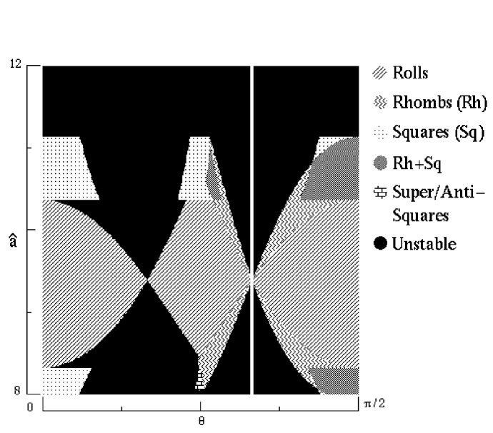
Figure 5: Square lattice bifurcation results (for various lattice angles $\theta$) as a function of the parameter $\hat{a}$ in the Lengyel-Epstein CIMA model (45). The diagram was generated by substituting the coefficient expressions from Appendix A into Table 1 and evaluating at different points in the $\hat{a}-\theta$ plane. The region near lattice angle $\theta=\pi/3$ has been removed, since this angle gives a hexagonal interaction,. Note also that at $\hat{a}\approx 9.4$ rolls are stable for all $\theta$. This value of $\hat{a}$ yields the degeneracy $\gamma=0$ in the hexagonal bifurcation problem (17).

We first consider the relative stability of patterns which lie on a square lattice. Figure 5 is a plot in the $(\theta,\hat{a})$ plane, generated by calculating the bifurcation coefficients $a_{1}$, $a_{2}=h(\pi/2)$, $a_{3}=h(\theta)$, and $a_{4}=h(\pi/2-\theta)$, as given in the Appendix. These coefficients are then substituted into the eigenvalue expressions in Table 1, generating the stability assignments in the figure. The region surrounding $\theta=\pi/3$ has been removed since $h(\theta)$ diverges as $\theta\to\pi/3$; the hexagonal lattice analysis is required at this point. Also, in the vicinity of $\theta=\pi/3$ the domain of validity of the bifurcation results is very small; certain slaved modes are only weakly damped, leading to a small-divisor problem in the computation of $h(\theta)$ (see Figure 6 for an example). Finally, we emphasize that anti- and super square patterns only exist for a discrete set of $\theta$ values, as discussed in Section 2.

Figure 6: Critical modes $(2,1)$ and $(-2,1)$ on a $(2,1)$-square lattice interact nonlinearly to generate a mode (0,2) that lies very near to the critical circle. We expect that this proximity will greatly reduce the domain of validity of the bifurcation calculation.

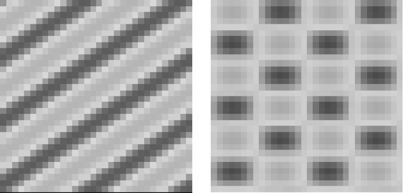
Figure 7: Rolls and Rhombs in Lengyel-Epstein CIMA model (45) for $\delta=1$, $\hat{b}=5$, and $\hat{c}$ chosen close to the Turing bifurcation point, as discussed in the text. Plot is of the numerically computed amplitude of the activator variable $u$, starting with a random initial condition. Rolls were generated at $\hat{a}=9.74$, rhombs at $\hat{a}=9.8$, in agreement with Figure 5. The computational domain corresponds to a (3,2)-square lattice; the grid size is $32\times 32$.

Figure 8: Unfolding of the degeneracy $(\hat{a}=9.39\ldots$) for the Lengyel-Epstein CIMA model. All other primary solution branches on the hexagonal lattices are unstable.

A number of general conclusions may be drawn from Figure 5. At all values of $\hat{a}$, simple squares are unstable for some range of $\theta$-values. We therefore conclude that they are unstable, near onset, in the unbounded domain. Rolls are similarly unstable for all $\hat{a}$ with the exception of $\hat{a}\approx 9.4$, where rolls are stable to perturbations in any direction $\theta$. Below we discuss the significance of this particular $\hat{a}$-value.

Figure 7 shows numerical simulations at two points in Figure 5. A square box size of $L=\sqrt{13}(2\pi/q_{c})$ gives critical lattice vectors of $(\pm 3,2)(2\pi/L)$ and $(\pm 2,3)(2\pi/L)$ (cf. Figure 1). A $(3,2)$-lattice generates mode angles of $\theta_{3}=\cos^{-1}12/13\approx\pi/8$ and $\theta_{4}=\pi/2-\theta_{3}\approx 3\pi/8$. Figure 5 suggests that for $\theta=3\pi/8$ rolls become unstable to rhombs at $\hat{a}\approx 9.8$. The rolls in Figure 7 were generated from random initial conditions at $\hat{a}=9.74$; the rhombs were generated from random initial conditions at $\hat{a}=9.8$. For these simulations $\delta=1$, $\hat{b}=5$, and the numerics were performed quite close to the bifurcation point, using a value of $K=K_{c}+2.9\times 10^{-4}$. These numerical results are in fact sensitive to the size and shape of the computational domain; the choice of the computational domain damps modes that might otherwise destabilize the rhombs.

In Figure 5, rolls appear to become stable for all $\theta$ at the point $\hat{a}\approx 9.4$. This is the point at which the hexagonal degeneracy condition $\gamma=0$ is satisfied; since the nonlinear terms differ by a constant, the only way to satisfy $\gamma\equiv\tilde{u}F_{2}(u_{1},v_{1})+\tilde{v}G_{2}(u_{1},v_{1})=0$ in this model is to take $F_{2}(u_{1},v_{1})=G_{2}(u_{1},v_{1})=0$, which occurs at

$$x_{0}^{2}=2+{\sqrt{21}\over 3}\Rightarrow\hat{a}=9.39\ldots.$$

At this point, hexagons are unstable to rolls (cf. Figure 2 for $\alpha=0$, $\beta<0$).

The results summarized by Table 2 may be used to determine certain aspects of the hexagonal bifurcation problems near the degeneracy $\gamma=0$. In section 4.1 it was pointed out that the unfolding scenario is fairly simple; in this model, the unfolding computation is even simpler. Since $F_{2}(u_{1},v_{1})=0$, the parameter $\alpha$ is zero. And since we know from section 4.1 that there is no $\theta$-dependence, the unfolding is described by the single bifurcation diagram given in Figure 8.

5.2 An Example of Super Squares

      

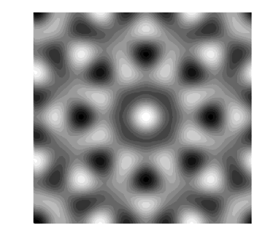
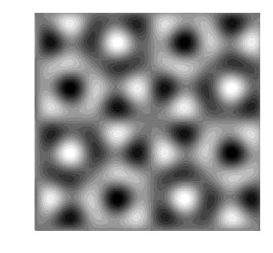
Figure 9: Examples of super squares and anti-squares for $(m,n)=(5,2)$, i.e. a box size of $\sqrt{29}(2\pi/q_{c})$. Patterns consist of four equal-amplitude critical Fourier modes, as described in section 2.

Section 2 described two types of superlattice patterns for square lattices: super squares and anti-squares. Figure 9 gives an example of each of these patterns for $(m,n)=(5,2)$, corresponding to $\theta_{3}=\cos^{-1}(20/29)$. Each pattern has a $\pi/2$ rotational symmetry. Super squares are invariant under reflections of the square domain; anti-squares have symmetries involving both translations and reflections (see [9] for details).

In Section 4 a system was constructed which supported stable super hexagons; by using the Appendix coefficient expressions, coupled with the stability information in Table 1, we may similarly construct a system which supports either super or anti-squares. (The relative stability of super and anti-squares is determined by terms of higher than cubic order in (15), which we have not computed.) The reaction-diffusion system (2.1) with

$$f(u,v) = au-1.8v-0.15uv+v^{2},$$

$$g(u,v) = 6u-2.8v+2.8v^{2}+0.2u^{3},$$ (49)

$$K = 9,$$

undergoes a Turing bifurcation at $a_{c}=1.8797\ldots$ with critical wave number $q_{c}=0.88563\ldots$. Figure 10 shows a numerical integration of this system at $a=1.88$, just above onset, showing both the initial condition and final steady state.

        

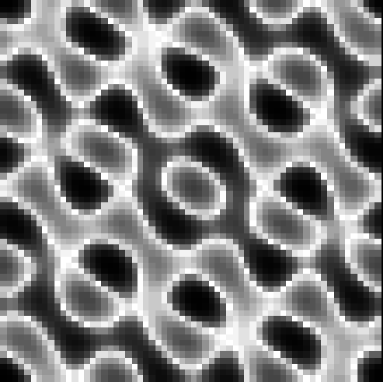
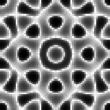
Figure 10: Numerical integration of system (5.2) described in Section 5.2, with a box of size $\sqrt{29}(2\pi/q_{c})$, and on a $64\times 64$ grid. The initial (left) and final (right) distributions of the field $u({\bf r})$ are shown. Compare the final state with the super squares of Figure 9.

6 Conclusions

From the general two-component reaction-diffusion system (2.1), we have derived analytic expressions for the coefficients of the leading nonlinear terms in the bifurcation equations for rhombic, square and hexagonal lattices. These coefficients allow us to calculate the relative stability of patterns which are periodic on either square lattices (stripes, squares, rhombs, and super squares or anti-squares) or hexagonal lattices (stripes, simple hexagons, rhombs, super hexagons or super triangles) at the onset of the Turing instability. In particular, the dependence of stability upon system parameters may be calculated explicitly for specific reaction-diffusion models, as we demonstrated for several model equations, including the Lengyel-Epstein CIMA model.

One of the surprising results of our general analysis is that details of the reaction-kinetics enter the computation of the bifurcation coefficients in a very limited fashion. In the case of the degenerate hexagonal bifurcation problem we show that the coefficients of the cubic terms in the bifurcation problem depend on the reaction-kinetics through just two effective parameters, that are simple to compute. Moreover, we find that at this degeneracy the angle dependence, which is expected for the rhombic lattice problems, drops out completely, and that rhombs and super hexagons never bifurcate stably at the Turing bifurcation point of two-component reaction-diffusion models. However, in the unfolding of this degenerate bifurcation problem we find that super hexagons may co-exist stably with simple hexagons and stripes for a limited range of the bifurcation parameter. This tri-stability property is demonstrated by numerical simulation of a reaction-diffusion system in the vicinity of the degenerate bifurcation point.

We plan to carry out more extensive numerical investigations that test some of the predictions of our bifurcation analysis. This will enable us to investigate the domain of validity of our bifurcation analysis, which is restricted to small-amplitude spatially-periodic Turing patterns. We also intend to determine the nature of the curious behavior at the hexagonal degeneracy, and to determine to what extent parameter collapse is exhibited by systems with three or more components, e.g. for Turing patterns in activator-inhibitor-immobilizer models [21].

7 Acknowledgments

We have benefited from discussions with E. Knobloch, H. Riecke, and A.C. Skeldon. The research of MS was supported by NSF grant DMS-9404266 and by an NSF CAREER award DMS-9502266.

Appendix A Appendix

Here we summarize our calculations of the coefficients in the bifurcation problems associated with rhombs and hexagons, for systems of the form

$$u_{t} = \nabla^{2}u+au+bv+F_{2}(u,v)+F_{3}(u,v)+\cdots$$

$$v_{t} = K\nabla^{2}v+cu+dv+G_{2}(u,v)+G_{3}(u,v)+\cdots,\quad\nabla^{2}=\partial_{xx}+\partial_{yy}.$$

The calculation assumes that the linear coefficients are near the Turing bifurcation point, i.e.,

$$a=a_{c}+\lambda_{a},\quad b=b_{c}+\lambda_{b},\quad c=c_{c}+\lambda_{c},\quad d=d_{c}+\lambda_{d},\quad K=K_{c}+\lambda_{K},$$

$$(K_{c}a_{c}-d_{c})^{2}+4K_{c}b_{c}c_{c}=0,$$

and that the system is in the Turing regime (conditions (9)). The following values are common to all coefficient expressions: the right and left null vectors from the linear problem,

$$\left(\matrix{u_{1}\cr v_{1}\cr}\right)\equiv\left(\matrix{-b_{c}\cr a_{c}-q_{c}^{2}\cr}\right),\quad\left(\matrix{\tilde{u}\cr\tilde{v}\cr}\right)\equiv\left(\matrix{c_{c}\cr-v_{1}\cr}\right);$$

the critical wave number $q_{c}$, where

$$q_{c}^{2}\equiv{K_{c}a_{c}+d_{c}\over 2K_{c}};$$

the quadratic and cubic nonlinearities from the Taylor expansion of the reaction terms,

$$\left(\matrix{F_{2}(u,v)\cr G_{2}(u,v)\cr}\right) \equiv \left(\matrix{f_{uu}u^{2}/2+f_{uv}uv+f_{vv}v^{2}/2\cr g_{uu}u^{2}/2+g_{uv}uv+g_{vv}v^{2}/2\cr}\right)$$

$$\vskip 6.0pt plus 2.0pt minus 2.0pt\left(\matrix{F_{3}(u,v)\cr G_{3}(u,v)\cr}\right) \equiv \left(\matrix{f_{uuu}u^{3}/6+f_{uuv}u^{2}v/2+f_{uvv}uv^{2}/2+f_{vvv}v^{3}/6\cr g_{uuu}u^{3}/6+g_{uuv}u^{2}v/2+g_{uvv}uv^{2}/2+g_{vvv}v^{3}/6\cr}\right);$$

and three effective parameters involving the quadratic and cubic nonlinearities,

$$\eta_{1} \equiv \tilde{u}{\partial F_{2}(u_{1},v_{1})\over\partial u_{1}}+\tilde{v}{\partial G_{2}(u_{1},v_{1})\over\partial u_{1}}$$

$$\eta_{2} \equiv \tilde{u}{\partial F_{2}(u_{1},v_{1})\over\partial v_{1}}+\tilde{v}{\partial G_{2}(u_{1},v_{1})\over\partial v_{1}}$$

$$\beta \equiv \tilde{u}F_{3}(u_{1},v_{1})+\tilde{v}G_{3}(u_{1},v_{1}).$$

The value of the linear term $\mu$ in the amplitude equations below is given by

$$\mu\equiv(\tilde{u},\tilde{v})\cdot\left(\matrix{\lambda_{a}&\lambda_{b}\cr\lambda_{c}&\lambda_{d}-q_{c}^{2}\lambda_{K}\cr}\right)\left(\matrix{u_{1}\cr v_{1}\cr}\right).$$

Finally, an overall factor of $u_{1}\tilde{u}+v_{1}\tilde{v}$, which is always positive, has been removed from the equations by rescaling time.

A.1 Rhombic lattice

The amplitude equation for the rhombic lattice problem is

$$\dot{z}_{1} = \mu z_{1}+a_{1}|z_{1}|^{2}z_{1}+h(\theta)|z_{\theta}|^{2}z_{1},$$

$$\dot{z}_{\theta} = \mu z_{\theta}+a_{1}|z_{\theta}|^{2}z_{\theta}+h(\theta)|z_{1}|^{2}z_{\theta}.$$

The coefficients are given by

$$a_{1}=(u_{2}+u_{5})\eta_{1}+(v_{2}+v_{5})\eta_{2}+3\beta,$$

$$h(\theta)=(u_{3}+u_{4}+u_{5})\eta_{1}+(v_{3}+v_{4}+v_{5})\eta_{2}+6\beta,$$

where

$$\left(\matrix{u_{2}\cr v_{2}\cr}\right)={1\over 9K_{c}q_{c}^{4}}\left(\matrix{4K_{c}q_{c}^{2}-d_{c}&b_{c}\cr c_{c}&4q_{c}^{2}-a_{c}\cr}\right)\left(\matrix{F_{2}(u_{1},v_{1})\cr G_{2}(u_{1},v_{1})\cr}\right),$$

$$\left(\matrix{u_{3}\cr v_{3}\cr}\right)={2\over\xi_{+}}\left(\matrix{K_{c}(a_{c}+2q_{c}^{2}\cos\theta)&b_{c}\cr c_{c}&{d_{c}\over K_{c}}+2q_{c}^{2}\cos\theta\cr}\right)\left(\matrix{F_{2}(u_{1},v_{1})\cr G_{2}(u_{1},v_{1})\cr}\right),$$

$$\left(\matrix{u_{4}\cr v_{4}\cr}\right)={2\over\xi_{-}}\left(\matrix{K_{c}(a_{c}-2q_{c}^{2}\cos\theta)&b_{c}\cr c_{c}&{d_{c}\over K_{c}}-2q_{c}^{2}\cos\theta\cr}\right)\left(\matrix{F_{2}(u_{1},v_{1})\cr G_{2}(u_{1},v_{1})\cr}\right),$$

$$\left(\matrix{u_{5}\cr v_{5}\cr}\right)={2\over K_{c}q_{c}^{4}}\left(\matrix{-d_{c}&b_{c}\cr c_{c}&-a_{c}\cr}\right)\left(\matrix{F_{2}(u_{1},v_{1})\cr G_{2}(u_{1},v_{1})\cr}\right),$$

with

$$\xi_{\pm}=K_{c}q_{c}^{4}(1\pm 2\cos\theta)^{2}.$$

It may be shown that

$$u_{3}+u_{4}+u_{5} = {2\over K_{c}q_{c}^{4}(1-4\cos^{2}\theta)^{2}}\biggl{(}F_{2}(u_{1},v_{1})\left(2K_{c}a_{c}-d_{c}(1+16\cos^{4}\theta)\right)$$

$$\qquad\qquad\qquad\qquad\quad+G_{2}(u_{1},v_{1})b_{c}(3+16\cos^{4}\theta)\biggr{)},$$

$$\vskip 6.0pt plus 2.0pt minus 2.0ptv_{3}+v_{4}+v_{5} = {2\over K_{c}q_{c}^{4}(1-4\cos^{2}\theta)^{2}}\biggl{(}F_{2}(u_{1},v_{1})c_{c}(3+16\cos^{4}\theta)$$

$$\qquad\qquad\qquad\qquad\quad+G_{2}(u_{1},v_{1})\left(2{d_{c}\over K_{c}}-a_{c}(1+16\cos^{4}\theta)\right)\biggr{)}.$$

A.2 Hexagonal lattice

The amplitude equation for the hexagonal lattice problem is

$$\dot{z}_{1}=\mu z_{1}+\gamma z_{2}^{*}z_{3}^{*}+b_{1}|z_{1}|^{2}z_{1}+b_{2}(|z_{2}|^{2}+|z_{3}|^{2})z_{1},$$

with $\dot{z}_{2}$ and $\dot{z}_{3}$ obtained by cyclically permuting $z_{1},z_{2},z_{3}$. The coefficients are given by

$$\gamma=2{\left(\tilde{u}F_{2}(u_{1},v_{1})+\tilde{v}G_{2}(u_{1},v_{1})\right)},$$

$$b_{1}=a_{1},$$

$$b_{2}=(u_{5}+u_{6})\eta_{1}+(v_{5}+v_{6}+v_{7})\eta_{2}-{\gamma\tilde{v}v_{7}\over u_{1}\tilde{u}+v_{1}\tilde{v}}+6\beta,$$

where $u_{1}$, $v_{1}$, $u_{5}$, and $v_{5}$ are given in the rhombic case, and

$$\left(\matrix{u_{6}\cr v_{6}}\right)={1\over 2K_{c}q_{c}^{4}}\left(\matrix{3K_{c}q_{c}^{2}-d_{c}&b_{c}\cr c_{c}&3q_{c}^{2}-a_{c}\cr}\right)\left(\matrix{F_{2}(u_{1},v_{1})\cr G_{2}(u_{1},v_{1})\cr}\right),$$

$$v_{7}={1\over b_{c}}\left({\gamma u_{1}\over u_{1}\tilde{u}+v_{1}\tilde{v}}-2F_{2}(u_{1},v_{1})\right).$$

References

- [1] A.M. Turing, Phil. Trans. R. Soc. London B 237 (1952) 37
- [2] A collection of review papers on Turing patterns can be found in: R. Kapral and K. Showalter (eds.), Chemical Waves and Patterns, Understanding Chemical Reactivity 10, Kluwer, Dordrecht (1995).
- [3] V. Castets, E. Dulos, J. Boissonade and P. De Kepper, Phys. Rev. Lett. 64 (1990) 2953
- [4] Q. Ouyang and H.L. Swinney, Nature 352 (1991) 610
- [5] Q. Ouyang, Z. Noszticzius and H.L. Swinney, J. Phys. Chem. 96 (1992) 6773.
- [6] I. Lengyel and I.R. Epstein, Science 251 (1991) 650
- [7] M. Golubitsky, I.N. Stewart and D.G. Schaeffer. Singularities and Groups in Bifurcation Theory: Vol. II. Appl. Math. Sci. Ser. 69. Springer-Verlag, New York (1988).
- [8] B. Dionne and M. Golubitsky, Z. Angew. Math. Phys. 43 (1992) 36
- [9] B. Dionne, M. Silber and A.C. Skeldon, Nonlinearity 10 (1997) 321
- [10] A.C. Skeldon and M. Silber, “New Stability Results for Patterns in a Model of Long Wavelength Convection”, Physica D (to appear) (1998).
- [11] M. Silber and M.R.E. Proctor, “Nonlinear Competition Between Small and Large Hexagonal Patterns”, preprint (1998).
- [12] A. Kudrolli, B. Pier and J.P. Gollub, “Superlattice Patterns in Surface Waves”, Physica D (to appear) (1998)
- [13] H. Othmer, Annals of NY Acad. Sci. 316 (1979) 64
- [14] T.K. Callahan and E. Knobloch, Nonlinearity 10 (1997) 1179.
- [15] T.K. Callahan and E. Knobloch, “Pattern Formation in Three-Dimensional Reaction-Diffusion Systems”, preprint (1998).
- [16] G. Gunaratne, Q. Ouyang and H.L. Swinney, Phys. Rev. E 50 (1994) 2802
- [17] V. Dufiet and J. Boissonade, J. Chem. Phys. 96 (1992) 664
- [18] A. De Wit, G. Dewel, P. Borckmans and D. Walgraef, Physica D 61 (1992) 289
- [19] A. Rovinsky and M. Menzinger, Physical Review A 46 (1992) 6315
- [20] O. Jensen, E. Mosekilde, P. Borckmans and G. Dewel, Physica Scripta 53 (1996) 243
- [21] J. E. Pearson, Physica A 188 (1992) 178