Secondary instabilities form a codimension–2 point accompanied by a homoclinic bifurcation

Abstract

A study of secondary instabilities in ac–driven electroconvection of a planarly aligned nematic liquid crystal is presented. At low frequencies one has a transition from normal rolls to a zig–zag pattern and at high frequencies a direct transition from normal to abnormal rolls. The crossover defines a codimension–2 point. This point is also the origin of a line of homoclinic bifurcations, which enable the transition from zig–zags to abnormal rolls at lower frequencies.

A large degree of universality has been found in primary instabilities leading to periodic patterns in spatially extended systems[1]. A full classification was achieved. For example, in axially anisotropic quasi–2D systems undergoing a steady supercritical bifurcation one can have at threshold either normal rolls (NRs), which orient according to the preferred direction, or oblique rolls, which occur in two symmetry–degenerate variants and may superpose to give rectangles [2].

A full classification of the secondary instabilities that may destabilize the primary patterns appears rather prohibitive, except in the quasi–1D case [3]. For Rayleigh-Bénard convection in simple fluids, the prime example for isotropic quasi–2D pattern formation, the relevant secondary instabilities generate the celebrated Busse balloon and have been analysed in detail [4]. By contrast, in the best studied axially anisotropic system, namely ac–driven electroconvection (EC) in planarly aligned nematic liquid crystal layers, the secondary instabilities arising when the main control parameter (the amplitude of the voltage) is increased have only recently been understood starting from the hydrodynamic equations [5]. It was found that in the range where one has NRs at threshold the well–known long–wave zig–zag (ZZ, or undulatory, or wavy) instability occurs only for frequencies $f$ (the second control parameter) below some value $f_{AR}$.

For $f>f_{AR}$ one should have a homogeneous instability. The nematic director, which near the primary threshold lies within the plane made up of the NR wave vector ($\parallel{\vec{x}}$) and the layer normal ($\parallel{\vec{z}}$), rotates out of this plane in one of two symmetry–equivalent directions. Since the director is anchored at the upper and lower plate along ${\vec{x}}$, this involves a twist deformation of the director field, and one may speak of a twist mode. The resulting roll pattern was termed ’abnormal rolls’ (ARs), following similar observations in EC with homeotropic anchoring [6]. Since homeotropic systems can be rotationally invariant or nearly so (in the presence of a weak planar magnetic field) the AR–transition can occur at or near threshold, allowing for a description of the scenario in terms of coupled Ginzburg–Landau equations [7]. However, one of the most interesting effects elucidated in Ref. [5], namely the restabilization of ARs above the ZZ–instability, is hardly expected under these conditions [7].

We here present a study of the predicted crossover from the ZZ– to the AR–transition in planar EC. Besides identifying experimentally this new type of codimension–2 (C2) point, we unravel the behavior in its neighborhood in the voltage–frequency plane experimentally and by a normal–form analysis involving two relevant modes. We show that at this C2–point a hitherto unsuspected line originates, which limits from above the regime where one may have ZZ–patterns. At this line one has an unusual type of homoclinic bifurcation from ZZs to ARs. A particularly interesting feature is the hysteresis found when this line is crossed from above. Then ARs persist down to a well–defined stability limit. The normal form shows that this class of two–mode scenario is of general importance, e.g. for certain types of line defects.

We perform experiments on EC in the conduction regime of the liquid crystal 4-methoxybenzylidene-4’-n-butylaniline (MBBA) at a temperature of $15^{o}C$. We use a channel geometry that is only moderately extended in the x–direction, namely a capacitor, where a $25\times 10\,mm$ ITO–coated glass plate faces another glass plate with a $L_{x}=315\,\mu m$ wide and $L_{y}\approx 10000\,\mu m$ stripe of ITO created by an etching process [8, 9]. The distance $d=24\,\mu m$ between the two plates scales the wavelength of the convection pattern, which arises when the amplitude $V$ of the driving ac–voltage passes a certain critical value $V_{c}$. A mechanical treatment of the surfaces (rubbing) fixes the planar orientation of the director almost perpendicular to the y–direction, which is defined by the lateral boundaries of the channel. The patterns are visualized by the standard shadowgraph technique [10] and detected using a microscope and a video–camera.

The left–hand side of Fig. 1 shows the NRs in the low frequency regime. They arise from the unstructured ground state via a primary instability, and destabilize at a higher voltage due to a secondary ZZ–instability. The resulting pattern is shown in the middle part. At an even higher voltage, ARs appear as shown in the right–hand side of Fig. 1. They look very similar to NRs—a special optical technique is needed in order to measure their underlying twist [11]. This image represents the first direct experimental observation of the ZZ–AR transition—presumably supported by the lateral boundaries—in EC in a planarly aligned liquid crystal.

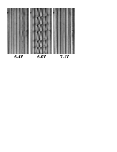
FIG. 1.: Convection patterns in a $315\,\mu m\times 1020\,\mu m$ part of the channel at 3 different ac–voltages at 43 Hz.

The procedure to obtain the five different relevant transitions in this scenario is illustrated in Fig. 2. The measurement of the primary instability is presented in the lower part. Here the light intensity modulation along the $x$–axis was analyzed by means of Fourier analysis. The intensity of the peak corresponding to the critical wave number is shown as a function of the driving voltage. This number is supposed to increase linearly with the distance from the threshold voltage $V_{c}$. The linear extrapolation of the data to zero determines the onset of convection. In our finite channel this bifurcation is imperfect [8, 9]. We have measured the intensity for increasing (open squares) and decreasing (solid circles) voltage: This transition has no hysteresis.

The angle of the ZZs with respect to the boundaries was measured by means of a correlation technique, at fixed position where this angle turned out to be maximal. This order parameter is shown in the middle row of Fig. 2. It is obvious that ZZs appear at a driving frequency of 43 Hz, but not at 80 Hz. The onset of ZZs at 43 Hz occurs at 6.55 V, as measured by means of a square–root extrapolation. The transition is imperfect and has no hysteresis. The transition from ZZs to ARs was determined with a threshold criterion (dotted line). It has a large hysteresis. The two points measured at the transition from ARs to ZZs are transients, which cannot be avoided within the pacing of 1 minute used here.

In order to determine the onset of ARs we have measured the twist angle by a special optical setup [11], which analyzes the ellipticity of the transmitted light and will be described in detail elsewhere [12]. The results are shown in the upper column of Fig. 2. The transition to ARs is easy to identify at the driving frequency of 80 Hz. An (imperfect) supercritical pitchfork bifurcation is indicated at a voltage of 7.2 V: The first direct experimental demonstration of the transition from NRs to ARs in EC.

At the driving frequency of 43 Hz the situation is more complicated. Here the ZZ–pattern mediates between the regime of NRs and ARs. The ZZs are accompanied by a twist. Thus the hysteresis in the ZZ–pattern manifests itself also in a hysteresis of the measured twist angle. The bifurcation from NRs to ARs can now be identified only indirectly, because both patterns are unstable with respect to ZZs in the vicinity of this bifurcation point. We thus measure these points by an extrapolation from the data obtained in the regime of ARs, assuming an imperfect bifurcation as indicated by the solid line.

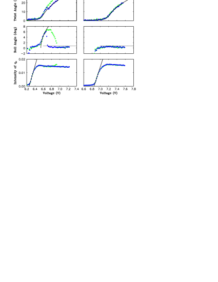
FIG. 2.: Measurements at two frequencies. Open squares (solid circles) correspond to increasing (decreasing)voltage. We show the twist angle (top), the zig-zag angle (middle), and the strength of convection (bottom). The solid lines are fits to determine the thresholds.

Fig. 3 is a stability diagram, which displays all five bifurcation lines discussed above. The crosses correspond to $V_{c}$. The open squares indicate the ZZ–instability. The solid squares (open diamands) mark the transition from ZZs to ARs (ARs to ZZs) taking place at increasing (decreasing) voltage. The solid circles indicate the bifurcation from NRs to ARs. In order to simplify a comparison with the theory, the same data are shown in the upper part of Fig. LABEL:ecread09.eps with a rescaled voltage, namely $\epsilon=V^{2}/V_{c}^{2}-1$. Note the similarity of this measurement with Fig. 3 of Ref.[5] (those calculations were done for a different material). The solid lines are least–square fits of data points above 67 Hz to the theory presented below.

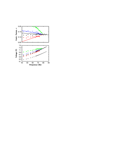
FIG. 3.: Experimental stability diagram. We show the threshold of convection (crosses), the ZZ–instability (open squares), the disappearance of ZZs for increasing voltage (solid squares), the destabilization of ARs for decreasing voltage (open diamonds), and the AR–instability (solid circles).

For a theoretical description of the scenario we adopt a phenomenological approach based on a Ginzburg-Landau expansion around the bifurcation from NRs to ARs in the vicinity of the C2 point. Let $\phi$ describe the (real) amplitude of the twist mode, which plays the role of the order parameter. The pre–bifurcation state sustains a spontaneous periodic pattern whose phase represents a soft (Goldstone) mode which has to be included in the description. We write the phase as $q{\hat{x}}+\vec{\nabla}\theta$, such that $q{\hat{x}}+\vec{\nabla}\theta$ is the local wave vector. Allowing only for variations along $y$ (as is adequate for the channel geometry) the Ginzburg-Landau equation for the pitchfork bifurcation from NRs to ARs is given by

$$\partial_{t}\phi=(\mu-g\phi^{2})\phi+K\partial_{y}^{2}\phi-\gamma(\partial_{y}\theta+P_{a}),$$ (1)

with positive $g$ and $K$ and (reduced) control parameter $\mu$. The last term describes the bias when the rolls are (slightly) oblique (the local roll angle is $\arctan(\partial_{y}\theta/q)$). We allowed for a misalignment between the rubbing direction ($\phi=0$) and the $x$–axis defined by the channel geometry. $\gamma$ must be chosen positive, so reorienting the rolls favors rotation of the director in the opposite sense [5]. From a fit to the experiment (Fig. 2, top right) one finds $\gamma g^{1/2}P_{a}=0.0011$. The dynamics of the phase modulation is governed by the equation

$$\partial_{t}\theta=\partial_{y}J,\ J=D(\partial_{y}\theta+P_{a})-(\nu+h\phi^{2}/3)\phi,$$ (2)

with positive $D$ and $h$ (as it turns out). The first term in $J$ describes ordinary phase diffusion, and the second expression represents the coupling to the twist mode. The nonlinear term is essential, because $\nu$ crosses zero in the region of interest.

Straight–roll solutions (normal or oblique) are characterized by $\phi=\phi_{s}~{}(=const.)$ and $\partial_{y}\theta=P~{}(=const.)$ and their stability is derived from the growth rate $\lambda=-\frac{1}{2}B+\sqrt{\frac{1}{4}B^{2}-C}$ of modes $\sim e^{\imath py}$, where $B=-\mu+3g\phi_{s}^{2}+(K+D)p^{2},\ C=[\gamma\nu-D\mu+3(gD+h\gamma/3)\phi_{s}^{2}]p^{2}+KDp^{4}$. For stability one needs $B>0$ and $C>0$. Thus, for NRs with $\phi_{s}=0$ and $P_{a}=0$, there is a homogeneous instability at $\mu=0$, leading to ARs and a long–wave ZZ–instability at $\mu=\mu_{zz}=S_{zz}\nu$ with $S_{zz}=\gamma/D$. For negative $\nu$ one first has the ZZ–instability and eqs. (1,2) indeed describe the observed crossover scenario, as indicated in Fig. LABEL:ecread19.eps, lines AR and ZZ. From the expression for $C$ one sees that a nonzero $\phi$ suppresses the ZZ–instability. For negative $\nu$ this effect leads to restabilization of ARs ($\phi_{AR}^{2}=\mu/g$) above the line $\mu=S_{rs}\nu$ with $S_{rs}=\frac{S_{zz}}{3S_{zz}/S_{hb}-2}$, $S_{hb}=-3g/h$, see Fig. 4, line RS.

FIG. 4.: Theoretical stability diagram for $S_{zz}/S_{hb}=-2/5$. Solid (dashed) lines are for $P_{a}=0$ ($\gamma g^{1/2}P_{a}=0.0011$).

We now analyse the scenario expected when $\mu$ is varied for negative $\nu$. For static solutions of (1,2) one has $J=const$. Eliminating $\partial_{y}\theta$ leads to

$$K\partial_{y}^{2}\phi=-(\mu-\mu_{zz})\phi+g^{\prime}\phi^{3}+S_{zz}J,$$ (3)

with $g^{\prime}=g(1-S_{zz}/S_{hb})$, which is integrable. Invoking the analogy of a point particle (coordinate $\phi$, time $y$) one sees that the bounded solutions are either constant or periodic. The channel geometry requires that rolls remain on the average oriented along $y$, so that the average of $\partial_{y}\theta$ is zero. From (2) one then has $J=DP_{a}-<(\nu+\frac{1}{3}h\phi^{2})\phi>$ ($<...>=$ spatial average).

First we look for ZZ–solutions in the case $P_{a}=0$, where $\phi$ oscillates symmetrically around zero ($J=0$). From (3) one gets a one–parameter family of periodic solutions above the ZZ–line (apart from phase shifts). In particular there is the homoclinic (or actually heteroclinic) limit where the solution degenerates to a widely spaced array of domain walls separating regions where $\phi$ approaches the constant solutions $\pm\phi_{zz}$ with $\phi_{zz}=\sqrt{(\mu-\mu_{zz})/g^{\prime}}$. The undulations observed under increase of the voltage are (presumably) approximated by this solution. The maximum value of the roll angle is given by $\arctan(p_{zz}/q)$ with $p_{zz}=\frac{h}{3Dg^{\prime 3/2}}(\mu-\mu_{zz})^{1/2}(\mu-\mu_{hb})$. The roll angle (and thereby the undulation) first increases with $\mu$ and then decreases, reaching zero at the line $\mu=\mu_{hb}=S_{hb}\nu$. There $\phi_{zz}$ coincides with $\phi_{AR}$ and one is left with an array of marginally stable domain walls separating AR–regions with alternating director twist. Above this line (and also for positive $\nu$) only moving domain walls exist stably (for details see [13]).

Therefore, when the line HB is reached, the domain walls annihilate pairwise, and a single–domain AR is established. From now on ARs persist under changes of the parameters until their stability limit is reached. The integration constant $J$ maintains the AR value $-(\nu+\frac{1}{3}h\phi_{AR}^{2})\phi_{AR}\ (=0$ at $\mu_{hb})$. Thus, on lowering $\mu$, ARs persist down to the line RS where a discontinuous ZZ–instability occurs, as observed. The twist angle in the ZZ–state is larger than in the coexisting ARs, in agreement with the experiment (Fig. 2, top left). The solid lines in Fig. 3 represent a five-parameter fit of 4 lines through a common intersection point (the C2 point) with slopes incorporating the relation $S_{rs}=\frac{S_{zz}}{3S_{zz}/S_{hb}-2}$. This relation is in fact invariant under the linear mapping that connect the control parameters $\mu$ and $\nu$ of the model with the experimental control parameters $\epsilon-\epsilon_{AR}$ and $f-f_{AR}$.

The observed asymmetry of the undulations can be accommodated by choosing $P_{a}\neq 0$. In Fig. 4 the corresponding scenario is shown (dashed lines). The ZZ–instability remains sharp, since translation invariance along $y$ remains intact. At the homoclinic bifurcation again $J=0$. Now the length of the shorter arms of the ZZs vanishes there. The selected wavelength of the observed ZZ undulations presumably results from the finite width of the channel [13].

The nature of the hysteresis found is actually quite unique. One ingredient, typical for pattern–forming systems, is the conservation of the number of periodic units (here ZZ–undulations) due to pinning at the boundary (here the short ends). Another ingredient is the unusual homoclinic bifurcation of ZZ patterns from ARs. We note that the ZZ–instability comes out naturally, which underscores its importance for EC. In fact, for many other nematics, like the one used in Ref. [5], the ZZ–instability line joins the primary bifurcation line at another significant C2–point, which separates the regimes where oblique and normal rolls appear at threshold.

In summary, two nontrivial qualitative features of the model are in accordance with the experimental data: A hysteretical transition between ZZs and ARs vanishes at the C2–point, and the width of this hysteresis decreases linearily with the distance from this point.

The model should be applicable to other instabilities exhibiting a similar symmetry. Candidates are line defects and some types of domain walls in the bend–Fréedricksz distorted state in nematics. Sometimes in these 1D extended structures the director can escape out of the symmetry plane, which may mimic the transition from NRs to ARs described by $\phi$. If the position of the line/wall is not fixed from outside it can be described by our phase variable $\theta$. In those cases where one has a potential (no dissipative driving) our model predicts $\gamma\nu<0$ so that the ZZ–instability always occurs first, which appears to be consistent with experiments [14]. The model is not applicable if the coupling terms between the two active modes vanish by symmetry, as is the case in Ising–Bloch–type transitions of domain walls [15]. We also remark that the validity of the model is restricted to the immediate neighborhood of the C2 point.

We thank C. Chevallard, W. Pesch, E. Plaut, A. G. Roßberg and R. Stannarius for discussions and help. Support by DFG through Re588/12 and EU through TMR network FMRX-CT96-0085 is gratefully acknowledged.

REFERENCES

- [1] M. C. Cross and P. C. Hohenberg, Rev. Mod. Phys. 65, 851 (1993).
- [2] L. Kramer and W. Pesch, in Pattern Formation in Liquid Crystals, eds. A. Buka and L. Kramer (Springer–Verlag, New York, 1996).
- [3] P. Coullet and G. Iooss, Phys. Rev. Lett. 64, 866 (1990).
- [4] F. H. Busse, Rep. Prog. Phys. 41, 1929 (1978).
- [5] E. Plaut et al., Phys. Rev. Lett. 79, 2367 (1997); E. Plaut and W. Pesch, Phys. Rev. E, in press.
- [6] H. Richter, A. Buka, and I. Rehberg, in Spatio-Temporal Patterns in Nonequilibrium Complex Systems, eds. P. E. Cladis and P. Palffy–Muhoray (Addison–Wesley Publishing Company, Reading, MA, 1994).
- [7] A. G. Roßberg et al., Phys. Rev. Lett. 76, 4729 (1996); A. G. Roßberg, Ph. D.–Thesis, U. of Bayreuth, 1997 (in English).
- [8] Y. Hidaka, K. Shimokawa, T. Nagaya, H. Orihara, and Y. Ishibashi, J. Phys. Soc. Jap. 63, 1698 (1994).
- [9] S. Rudroff and I. Rehberg, Phys. Rev. E 55, 2742 (1997).
- [10] I. Rehberg, F. Hörner, and G. Hartung, J. Stat. Phys. 64, 1017 (1991).
- [11] T. J. Scheffer and J. Nehring, J. Appl. Phys. 56, 908 (1984); R. Stannarius, priv. communication.
- [12] S. Rudroff, V. Frette and I. Rehberg, submitted to PRE.
- [13] H. Zhao and L. Kramer, in preparation.
- [14] Y. Gabune, J. Itona, and L. Liebert, J. Phys. France 49, 681 (1988); C. Chevallard, M. Nobili, and J. M. Gilli, private communication.
- [15] P. Coullet et al., Phys. Rev. Lett. 65, 1352 (1990); T. Frisch et al., Phys. Rev. Lett. 72, 1471 (1994).