Spike autosolitons in the Gray-Scott model

Abstract

We performed a comprehensive study of the spike autosolitons: self-sustained solitary inhomogeneous states, in the classical reaction-diffusion system — the Gray-Scott model. We developed singular perturbation techniques based on the strong separation of the length scales to construct asymptotically the solutions in the form of a one-dimensional static autosolitons, higher-dimensional radially-symmetric static autosolitons, and two types of traveling autosolitons. We studied the stability of the static autosolitons in one and three dimensions and analyzed the properties of the static and the traveling autosolitons.

132E 1326

1 Introduction

Self-organization and pattern formation in nonequilibrium systems are among the most fascinating phenomena in nonlinear physics [1, 2, 3, 4, 5, 6, 7, 8, 9, 10, 11]. Pattern formation is observed in various physical systems including aero- and hydrodynamic systems; gas and electron-hole plasmas; various semiconductor, superconductor and gas-discharge structures; some ferroelectric, magnetic and optical media; combustion systems (see, for example, [5, 9, 10, 11, 12, 13, 14]), as well as in many chemical and biological systems (see, for example, [1, 2, 3, 4, 5, 6, 7, 15]).

Self-organization is often associated with the destabilization of the uniform state of the system [1, 2, 5, 10, 11]. At the same time, when the uniform state of the system is stable, by applying a sufficiently strong perturbation one can excite large-amplitude patterns, including autosolitons (ASs) — self-sustained solitary inhomogeneous states [8, 9, 10, 11, 16, 17, 18, 19]. Autosolitons are the elementary objects in open dissipative systems away from equilibrium. They share the properties of both solitons and traveling waves (or autowaves, as they are also referred to [2, 6]). They are similar to solitons since they are localized objects whose existence is due to the nonlinearities of the system. On the other hand, from the physical point of view they are essentially different from solitons in that they are dissipative structures, that is, they are self-sustained objects which form in strongly dissipative systems as a result of the balance between the dissipation and pumping of energy or matter. This is the reason why, in contrast to solitons, their properties are independent of the initial conditions and are determined primarily by the nonlinearities of the system [8, 9, 10, 11]. ASs can be static, pulsating, or traveling. As a result of their various instabilities, these simplest localized patterns can spontaneously transform into complex space-filling static or dynamic patterns, including complex pulsating and traveling patterns, or spatio-temporal chaos [8, 9, 10, 11, 12, 13, 14, 18, 19, 20, 21, 22, 23, 24, 25, 26, 27, 28, 29, 30, 31, 32, 33]. Thus, it is the destabilization of the ASs that is the main source of self-organization in nonequilibrium systems with the stable homogeneous state.

Real physical, chemical, and biological systems exhibiting pattern formation and self-organization are extremely complicated, so simplified models are used to describe these phenomena. A prototype model of this kind is a pair of reaction-diffusion equations of the activator-inhibitor type

$$\tau_{\theta}\frac{\partial\theta}{\partial t} = l^{2}\Delta\theta-q\left(\theta,\eta,A\right),$$ (1.1)

$$\tau_{\eta}\frac{\partial\eta}{\partial t} = L^{2}\Delta\eta-Q\left(\theta,\eta,A\right),$$ (1.2)

where $\theta$ is the activator, $\eta$ is the inhibitor, $\tau_{\theta}$, $l$ and $\tau_{\eta}$, $L$ are the time and the length scales of the activator and the inhibitor, respectively; $A$ is the control (bifurcation) parameter; $q$ and $Q$ are certain nonlinear functions representing the activation and the inhibition processes. Examples of these equations for various physical systems are given in [9, 10, 11, 12, 13, 25] where the physical meaning of the variables $\theta$ and $\eta$ and the nature of the activation and the inhibition processes are discussed. The well-known Brusselator [1] and the Gray-Scott [34] models of autocatalytic chemical reactions, the classical Gierer-Meinhardt model of morphogenesis [35], the FitzHugh-Nagumo [36] and the piecewise-linear Rinzel-Keller model [37] for the propagation of pulses in the nerve fibers are all special cases of Eqs. (1.1) and (1.2).

The fact that $\theta$ is the activator means that for certain parameters the uniform fluctuations of $\theta$ will grow when the value of $\eta$ is fixed. From the mathematical point of view, this is given by the condition [9, 10, 11, 18]

$$q^{\prime}_{\theta}<0$$ (1.3)

for certain values of $\theta$ and $\eta$. On the other hand, the fact that $\eta$ is the inhibitor means that its own fluctuations decay and that it damps the fluctuations of the activator. Mathematically, these conditions are expressed by [9, 10, 11, 18]

$$Q^{\prime}_{\eta}>0,~{}~{}~{}q^{\prime}_{\eta}Q^{\prime}_{\theta}<0$$ (1.4)

for all values of $\theta$ and $\eta$, provided that the derivatives in Eq. (1.4) do not change sign.

Kerner and Osipov showed [8, 9, 10, 11, 16, 17, 18, 25] that the properties of the patterns and the self-organization scenarios in systems described by Eqs. (1.1) and (1.2) are chiefly determined by the parameters $\epsilon\equiv l/L$ and $\alpha\equiv\tau_{\theta}/\tau_{\eta}$ and the shape of the nullcline of the equation for the activator, that is, the dependence $\eta(\theta)$ given by the equation $q(\theta,\eta,A)=0$ for $A={\mathrm{c}onst}$. They demonstrated that depending on the shape of the activator nullcline all systems involved can be divided into two fundamentally different classes: N-systems, for which the nullcline is N- or inverted N-shaped and, $\Lambda$- or V-systems, for which the nullcline is $\Lambda$- or V-shaped, respectively (see Fig. 1).

Figure 1: Two qualitatively different types of the nullclines of Eqs. (1.1) and (1.2): N-systems (a) and $\Lambda$-systems (b).

Most works devoted to the description of pattern formation on the basis of Eqs. (1.1) and (1.2) deal with N-systems. In N-systems the equation $q(\theta,\eta,A)=0$ has three roots: $\theta_{1},\theta_{2},$ and $\theta_{3}$, for given values of $A$ and $\eta$. The roots $\theta_{1}$ and $\theta_{3}$ correspond to the stable states and $\theta_{2}$ corresponds to the unstable state in the system with $\eta={\mathrm{c}onst}$. It is easy to see that the FitzHugh-Nagumo and the piecewise-linear models belong to N-systems. For these models it was proved [27, 37] that Eqs. (1.1) and (1.2) with $L=0$ and $\alpha=\tau_{\theta}/\tau_{\eta}\ll 1$ have solutions in the form of the traveling waves (also called autowaves [2, 6], or traveling ASs [8, 9, 10, 11]). In [16, 17, 18, 19] it was shown that in another limit $L\gg l$ (or, more precisely, when $\epsilon=l/L\ll 1$ and $\alpha\gtrsim 1$) Eqs. (1.1) and (1.2) admit solutions in the form of the stable static patterns including ASs (see also [9, 10, 11]). Furthermore, it was shown that in systems with $\epsilon\ll 1$ and $\alpha\ll 1$ one can excite static, pulsating, and traveling patterns [8, 9, 10, 11, 18, 25, 28, 29, 30, 31, 32, 33]. The characteristic velocity of the traveling patterns in N-systems does not exceed the value of order $l/\tau_{\theta}$ [9, 11, 18, 27].

It is important to emphasize that $\epsilon$ or $\alpha$ are the natural small parameters in these system. Their smallness is in fact a necessary condition for the feasibility of any patterns [9, 10, 11]. Indeed, if the inverse were true, that is, if both the characteristic time and length scales of the variation of the inhibitor were much smaller than those of the activator, the inhibitor would easily damp all the deviations of the activator from the homogeneous steady state, making the formation of any kinds of persistent patterns impossible. On the other hand, the fact that we must have either $\epsilon\lesssim 1$ or $\alpha\lesssim 1$ implies that it is advantageous to consider the extreme cases of $\epsilon\ll 1$ or $\alpha\ll 1$. These conditions, in turn, will result in a significant simplification of the original highly nonlinear problem. Recently, this kind of approach has been successfully applied to a variety of problems (see, for example, [38]).

In N-systems with $\epsilon\ll 1$ the static ASs and other patterns are essentially the domains of high and low values of the activator separated by the interfaces (walls) where $\theta$ varies sharply over a distance of order $l$ from one stable state $\theta_{1}$ to the other $\theta_{3}$. The characteristic size ${\mathcal{L}}_{s}$ of these domain patterns lies in the range $l\ll{\mathcal{L}}_{s}\lesssim L$ and their amplitude (the value $\theta_{1}-$ $\theta_{3}$) is determined by the form of $q$ and $Q$ and becomes independent of $\epsilon$ as $\epsilon\rightarrow 0$ [9, 10, 11, 17, 18, 19, 20, 21, 22]. The properties of these patterns are essentially determined by the dynamics of their interfaces and the interaction between them. So, the majority of the theoretical work devoted to the description of the complex domain patterns in N-systems in fact developed an interfacial dynamics approach [9, 10, 11, 17, 18, 19, 20, 21, 22, 23, 24, 25, 29, 30, 31, 32, 33, 39, 40, 41]. On the basis of this approach, Kerner and Osipov developed a theory of instabilities of the domain patterns in the general N-systems in one dimension [8, 9, 10, 11]. More recently, we extended this theory for arbitrary domain patterns in higher-dimensional systems and extensively studied various pattern formation scenarios in these systems [21, 22, 40, 41].

At the same time, there are many physical, chemical and biological systems for which the activator nullcline is $\Lambda$- or V-shaped [Fig. 1(b)]. In this case the equation $q(\theta,\eta,A)=0$ for given $A$ and $\eta$ has only two roots: $\theta_{1}$ corresponding to the stable state, and $\theta_{2}$ corresponding to the unstable state in the system with $\eta={\mathrm{c}onst}$ [9, 10, 11, 16]. Among $\Lambda$-systems are many semiconductor and gas discharge structures, electron-hole and gas plasmas, radiation heated gas mixtures (see, for example, [9, 10, 11, 12, 16, 25]). It is not difficult to see that the Brusselator and the Gray-Scott models are $\Lambda$-systems, and the Gierer-Meinhardt model is a V-system.

Kerner and Osipov qualitatively showed that in $\Lambda$-systems the so-called spike ASs and more complex spike patterns can be excited [9, 11, 16, 42, 43]. They were the first to analyze the static spike ASs and strata in the Brusselator, the Gierer-Meinhardt model, and the electron-hole plasma [16, 42]. They found that when $\epsilon\ll 1$ and $\alpha\gtrsim 1$, the one-dimensional static spike AS can have small size of order $l$ and huge amplitude which goes to infinity as $\epsilon\rightarrow 0$. Dubitskii, Kerner, and Osipov formulated the asymptotic procedure for finding the stationary solutions in $\Lambda$-systems for sufficiently small $\epsilon$ [11, 42]. Recently, we showed that in another limiting case $\alpha\ll 1$ and $\epsilon\gg 1$ one can excite the one-dimensional traveling spike AS which also has small size and whose amplitude goes to infinity as $\alpha\rightarrow 0$ [44]. We also showed that, in contrast to the traveling patterns in N-systems, the velocity of this one-dimensional traveling spike AS can have huge values ($c\gg l/\tau_{\theta}$) and that the inhibitor distribution varies stepwise in the front of the spike. Thus, one can see that the properties of the spike patterns forming in $\Lambda$-systems differ fundamentally from those of the domain patterns forming in N-systems. In particular, since the interface connecting the two stable states at $\eta={\mathrm{c}onst}$ does not exist in $\Lambda$- systems, the size of the spike should be of the order of the smallest system length scale. For this reason, the concept of the interfacial dynamics developed for the domain patterns in N-systems is generally inapplicable to the description of spike patterns. Some properties of the one-dimensional static spike ASs and the main types of their instabilities in the simplified version of the Gray-Scott model have recently been studied by Osipov and Severtsev [45].

Spike patterns including the spike ASs are observed experimentally in the nerve tissue [46], chemical reactions [5, 47], electron-hole plasma [48], gas-discharge structures [49], as well as numerically in the simulations of the Brusselator, the Gierer-Meinhardt, and the Gray-Scott models [1, 15, 26, 35, 50]. At the same time, there is a only a limited number of theoretical studies of these patterns. Moreover, many aspects of these patterns including the stability of the spike ASs and their properties in higher dimensions as well as the spontaneous transitions between the static, the pulsating and the traveling spike ASs have not been studied at all. So far, there have been no general methods for dealing with spike patterns.

In the present paper we develop asymptotic methods for the description of the spike patterns and study their major properties in arbitrary dimensions as well as their shape and stability. We find the conditions of the spontaneous transitions between different types of the spike ASs and study the scenarios of the formation of the spike ASs and more complex spike patterns in one- and two-dimensional systems. To be specific, we consider the Gray-Scott model of an autocatalytic chemical reaction, which possesses a number of advantages. First, it is one of the rarest models for which in many cases one can obtain exact results. Second, a lot of the numerical studies of this model were performed recently [15, 26, 50, 51]. Finally, the Gray-Scott model possesses a particularly simple set of nonlinearities, so one can expect a certain degree of universality in the pattern formation scenarios exhibited by it.

The outline of our paper is as follows. In Sec. 2 we introduce the model we will study, in Sec. 3 we asymptotically construct the one-dimensional static AS, and the two- and the three-dimensional radially-symmetric ASs, in Sec. 4.1 we asymptotically construct the solutions in the form of the two types of traveling spike ASs, in Sec. 5 we analyze the stability of the one-dimensional and the higher-dimensional radially-symmetric static ASs and show the existence of various instabilities, in Sec. 6 we compare our results with the numerical simulations of the one-dimensional system, and in Sec. 7 we do that for the two-dimensional system, in Sec. 8 we discuss the works of other authors on the Gray-Scott model in light of our results, and in Sec. 9 we give the summary of our work and draw conclusions.

2 The model

The Gray-Scott model describes the kinetics of a simple autocatalytic reaction in an unstirred flow reactor. The reactor is a narrow space between two porous walls. Substance $Y$ whose concentration is kept fixed outside of the reactor is supplied through the walls into the reactor with the rate $k_{0}$ and the products of the reaction are removed from the reactor with the same rate. Inside the reactor $Y$ undergoes the reaction involving an intermediate species $X$:

$$2X+Y \stackrel{{\scriptstyle k_{1}\ }}{{\rightarrow}} 3X,$$ (2.1)

$$X \stackrel{{\scriptstyle k_{2}\ }}{{\rightarrow}} {\mathrm{i}nert}.$$ (2.2)

The first reaction is a cubic autocatalytic reaction resulting in the self-production of species $X$; therefore, $X$ is the activator species. On the other hand, the production of $X$ is controlled by species $Y$, so $Y$ is the inhibitor species. The equations of chemical kinetics which describe the spatiotemporal variations of the concentrations of $X$ and $Y$ in the reactor and take into account the supply and the removal of the substances through the porous walls take the following form [34]:

$${\partial X\over\partial t} = -(k_{0}+k_{2})X+k_{1}X^{2}Y+D_{X}\Delta X,$$ (2.3)

$${\partial Y\over\partial t} = k_{0}(Y_{0}-Y)-k_{1}X^{2}Y+D_{Y}\Delta Y,$$ (2.4)

where now $X$ and $Y$ are the concentrations of the activator and the inhibitor species, respectively, $Y_{0}$ is the concentration of $Y$ in the reservoir, $\Delta$ is the two-dimensional Laplacian, and $D_{X}$ and $D_{Y}$ are the diffusion coefficients of $X$ and $Y$.

In order to be able to understand various pattern formation phenomena in a system of this kind, it is crucial to introduce the variables and the time and length scales that truly represent the physical processes acting in the system. The first and the most important is the choice of the characteristic time scales. These are primarily dictated by the time constants of the dissipation processes. For $Y$ this is the supply and the removal with the rate $k_{0}$, whereas for $X$ this is the removal from the system and the decay via the second reaction with the total rate $k_{0}+k_{2}$. The natural way to introduce the dimensionless inhibitor concentration is to scale it with $Y_{0}$. Since we want to fix the time scale of the variation of the inhibitor (with the fixed activator), we will rescale $X$ in such a way that the reaction term in Eq. (2.4) will generate the same time scale as the dissipative term. This leads to the following dimensionless quantities:

$$\theta=X/X_{0},~{}~{}~{}\eta=Y/Y_{0},~{}~{}~{}X_{0}=\left({k_{0}\over k_{1}}\right)^{1/2}.$$ (2.5)

The characteristic time and length scales for these quantities are

$$\tau_{\theta}=\left(k_{0}+k_{2}\right)^{-1}, \tau_{\eta}=k_{0}^{-1},$$ (2.6)

$$l=\left(D_{X}\tau_{\theta}\right)^{1/2},~{} L=\left(D_{Y}\tau_{\eta}\right)^{1/2}.$$ (2.7)

Naturally, one should require the positivity of $\theta$ and $\eta$.

If we now write Eqs. (2.3) and (2.4) in the dimensionless form, we will arrive at the following set of equations:

$$\tau_{\theta}{\partial\theta\over\partial t} = l^{2}\Delta\theta+A\theta^{2}\eta-\theta,$$ (2.8)

$$\tau_{\eta}{\partial\eta\over\partial t} = L^{2}\Delta\eta-\theta^{2}\eta+1-\eta,$$ (2.9)

where we introduced a dimensionless parameter

$$A={Y_{0}k_{0}^{1/2}k_{1}^{1/2}\over(k_{0}+k_{2})}.$$ (2.10)

One can see from Eqs. (2.8) and (2.9) that $\tau_{\theta}$ and $\tau_{\eta}$ are in fact the characteristic time scales, and $l$ and $L$ the characteristic length scales of the variation of small deviations of $\theta$ and $\eta$ from the stationary homogeneous state $\theta=\theta_{h}$ and $\eta=\eta_{h}$:

$$\theta_{h}=0,~{}~{}~{}\eta_{h}=1.$$ (2.11)

Thus, the system is characterized by only three dimensionless parameters: $\alpha\equiv\tau_{\theta}/\tau_{\eta}$, $\epsilon\equiv l/L$, and $A$. As can be seen from Eq. (2.8), the parameter $A$ is the dimensionless strength of the activation process, that is, it describes the degree of deviation of the system from thermal equilibrium. With all this, Eqs. (2.8) and (2.9) are reduced to the form of Eqs. (1.1) and (1.2). Notice that the system given by Eqs. (2.8) and (2.9) is indeed a system of the activator-inhibitor type: the condition in Eq. (1.3) is satisfied for $\theta>\frac{1}{2A\eta}$, and the conditions in Eq. (1.4) are satisfied with $q^{\prime}_{\eta}<0$ and $Q^{\prime}_{\theta}>0$ for all $\theta>0$ and $\eta>0$.

The nullclines of Eqs. (2.8) and (2.9) are shown in Fig. 2.

Figure 2: The nullclines of Eqs. (2.8) and (2.9) for $A=1$ (a) and $A=3$ (b).

From this figure one can see that the nullcline of the equation for the activator has degenerate $\Lambda$-form. It consists of two separate branches: $\theta=0$ and $\theta={1\over A\eta}$. One can easily check that for $0<A<2$ there is only one stationary homogeneous state given by Eq. (2.11), whereas for $A>2$ two extra stationary homogeneous states exist

$$\theta_{h2,3}={A\mp\sqrt{A^{2}-4}\over 2},~{}~{}~{}\eta_{h2,3}={A\pm\sqrt{A^{2}-4}\over 2A}.$$ (2.12)

The stability analysis of these homogeneous states shows that for $\epsilon\ll 1$ or $\alpha\ll 1$ the homogeneous state $\theta=\theta_{h2}$, $\eta=\eta_{h2}$ is always unstable. For $\epsilon\ll 1$ the homogeneous state $\theta=\theta_{h3}$, $\eta=\eta_{h3}$ is unstable with respect to the Turing instability if $A<0.41\epsilon^{-1}$. For $\alpha\ll 1$ it is unstable with respect to the homogeneous oscillations (Hopf bifurcation) if $0.41\alpha^{-1/2}<A<\alpha^{-1/2}$, or it is an unstable node if $A<0.41\alpha^{-1/2}$. On the other hand, the homogeneous state $\theta=\theta_{h}$, $\eta=\eta_{h}$ is stable for all values of the system’s parameters. The latter is simple to understand: in order for the reaction to begin there has to be at least some amount of the activator put in at the start. Equivalently, the fact that the homogeneous state in Eq. (2.11) is stable for all values of the parameter $A$ (for an arbitrary deviation from thermal equilibrium) is the consequence of the degeneracy of the nullcline of Eq. (2.8). Thus, self-organization associated with the Turing instability of the homogeneous state $\theta_{h}=0$ and $\eta_{h}=1$ is not realized in the Gray-Scott model. In such a stable homogeneous system any inhomogeneous pattern, including the ASs, can only be excited by a sufficiently strong localized stimulus. In turn, self-organization will occur as a result of the instabilities of the large-amplitude patterns already present in the system.

Note that in the opposite case $\epsilon\gg 1$ and $\alpha\gg 1$ the dynamics of the system becomes dramatically simpler. Indeed, if we put both $L$ and $\tau_{\eta}$ to zero, from Eq. (2.9) we get a local relationship $\eta={1\over 1+\theta^{2}}$. Substituting this back to Eq. (2.8), we obtain

$$\tau_{\theta}{\partial\theta\over\partial t}=l^{2}\Delta\theta+{A\theta^{2}\over 1+\theta^{2}}-\theta.$$ (2.13)

This equation possesses a simple variational structure

$$\tau_{\theta}{\partial\theta\over\partial t}=-{\delta{\mathcal{F}}\over\delta\theta},~{}~{}~{}~{}{\mathcal{F}}=\int d^{d}x\left({l^{2}(\nabla\theta)^{2}\over 2}-A\theta+A\arctan\theta+{\theta^{2}\over 2}\right).$$ (2.14)

For $A<2$ the functional $\mathcal{F}$ has a unique global minimum at $\theta=\theta_{h}=0$, so any initial condition will relax to the homogeneous state $\theta_{h}$. For $A>2$ there are two stable homogeneous states $\theta=\theta_{h}$ and $\theta=\theta_{h3}$ (see above), so it is possible to have the waves of switching from one homogeneous state to the other [5]. It is easily checked that for $2<A<2.18$ the dominant homogeneous state is $\theta_{h}$, while for $A>2.18$ the dominant homogeneous state is $\theta_{h3}$.

In the case of $\epsilon\ll 1$ and $\alpha\ll 1$ the largest length scale in the system is $L$ and the longest time scale is $\tau_{\eta}$, so it is natural to scale length and time with $L$ and $\tau_{\eta}$, respectively. In these units Eqs. (2.8) and (2.9) will take the following form:

$$\alpha{\partial\theta\over\partial t}=\epsilon^{2}\Delta\theta+A\theta^{2}\eta-\theta,$$ (2.15)

$${\partial\eta\over\partial t}=\Delta\eta-\theta^{2}\eta+1-\eta.$$ (2.16)

We will assume that the problem is defined on the sufficiently large domain with neutral boundary conditions. Notice that the kinetic model used to arrive at Eqs. (2.15) and (2.16) imposes a restriction $\alpha\leq 1$ [see Eq. (2.6)]. Also, in the derivation we assumed that the system is essentially two-dimensional. For the sake of generality, in the following we will allow $\alpha$ to take arbitrary values and will work with the arbitrarily-dimensional Gray-Scott model.

3 Static spike autosolitons

Let us now study the simplest possible stationary pattern in the Gray-Scott model — the static spike AS. According to the general qualitative theory, these ASs form in $\Lambda$-systems when $\epsilon\ll 1$ [9, 10, 11, 16]. The condition $\epsilon\ll 1$ will therefore be assumed throughout this section.

3.1 One-dimensional static spike autosoliton

We begin with the analysis of the one-dimensional static spike AS. In the Gray-Scott model it is described by the following equations

$$\epsilon^{2}{d^{2}\theta\over dx^{2}}+A\theta^{2}\eta-\theta=0,$$ (3.1)

$${d^{2}\eta\over dx^{2}}-\theta^{2}\eta+1-\eta=0.$$ (3.2)

Since $\epsilon\ll 1$, there is a strong separation of the length scales in the AS [9, 10, 11, 16]. One can separate the spike region where the distribution of $\theta$ varies on the length scale of $\epsilon$, and the periphery of the AS where $\eta$ decays into the homogeneous state $\eta_{h}=1$ on the length scale of order 1. One can use this separation of the length scales to construct a singular perturbation theory which describes the distributions in the form of the static one-dimensional spike AS [42]. But before we do that, it is instructive to use a more qualitative approach which will give us an idea about the scaling of the main parameters of the AS and its qualitative shape. As will be seen below, this approach works when $\epsilon^{1/2}\lesssim A\ll 1$.

3.1.1 Case $A\sim\epsilon^{1/2}$: autosoliton collapse

According to this approach [9, 10, 11, 16], one assumes that the value of $\eta$ inside the spike (on the length scale of $\epsilon$) is close to a constant. This is a reasonable assumption as long as $\eta\gg\epsilon$ in the spike since the characteristic length scale of the variation of $\eta$ is 1. Let us denote this constant value of $\eta$ as $\eta_{s}$. Then, Eq. (3.1) with $\eta=\eta_{s}$ can be solved exactly. Its solution has the form

$$\theta(x)=\theta_{m}\cosh^{-2}\left({x\over 2\epsilon}\right){\mathrm{~{}}with~{}}\theta_{m}=\frac{3}{2A\eta_{s}}.$$ (3.3)

On the other hand, the distribution of $\theta$ given by Eq. (3.3) acts in Eq. (3.2) as a $\delta$-function, so away from the spike the distribution of $\eta$ is given by

$$\eta(x)=1-{3\epsilon\over\eta_{s}A^{2}}\e^{-|x|}.$$ (3.4)

Now, matching this solution for $\eta(x)$ with the condition that $\eta(0)=\eta_{s}$, we obtain the following expressions

$$\theta_{m}=\frac{3A}{A_{b}^{2}}\left[1\pm\sqrt{1-{A_{b}^{2}\over A^{2}}}~{}\right],~{}~{}\eta_{s}=\frac{A_{b}^{2}}{2A^{2}}\left[1\pm\sqrt{1-{A_{b}^{2}\over A^{2}}}~{}\right]^{-1},$$ (3.5)

where

$$A_{b}=\sqrt{12\epsilon}.$$ (3.6)

Note that these results were also obtained in [51] by applying Melnikov analysis to Eqs (3.1) and (3.2). Similar results for the simplified version of the Gray-Scott model were obtained in [45].

From Eq. (3.6) one can see that at $A<A_{b}$ the solution in the form of the spike AS does not exist. When $A>A_{b}$ there are two solutions: the one corresponding to the plus sign has larger amplitude and the one corresponding to the minus sign has smaller amplitude. As was shown by Kerner and Osipov, the solutions that have smaller amplitude are always unstable [9, 10, 11], so the only interesting solution corresponds to the plus sign in Eq. (3.5). This solution is precisely the static spike AS. The numerical simulations of Eqs. (2.15) and (2.16) show that if the value of $A$ is lowered, at $A=A_{b}$ a stable one-dimensional static spike AS collapses into the homogeneous state (see Sec. 6).

Let us look more closely at the parameters of the static spike AS and the conditions of validity of the approximations made in the preceding paragraphs. As can be seen from Eqs. (3.3) and (3.4), the distribution of the activator indeed has a form of the spike whose characteristic width is of order $\epsilon$, and the distribution of the inhibitor varies on the much larger length scale of order 1. Also, according to Eq. (3.5), the amplitude of the spike at $A$ close to $A_{b}$ is of order $\epsilon^{-1/2}\gg 1$ (and can in fact have huge values as $\epsilon$ gets smaller) and grows as the value of $A$ increases. At $A\sim 1$ the amplitude $\theta_{m}\sim\epsilon^{-1}$. These features fundamentally differ the AS forming in $\Lambda$-systems from the AS in N-systems.

Recall that in the derivation we neglected the variation of the inhibitor inside the spike. Since the characteristic length of the variation of $\eta$ is of order 1, this means that the value of $\eta=\eta_{s}$ in the center of the AS must be much greater than $\epsilon$. According to Eq. (3.5), this is indeed the case as long as $A\ll 1$, so the solution obtained above is a good approximation to the actual solution in this case. Also, in this case one can easily calculate the distribution of $\eta$ in the spike. To do this, we note that, according to Eq. (3.5), for $A\ll 1$ we have $\theta^{2}\eta\gg 1$ in the spike, so the last two terms in Eq. (3.2) can be neglected. Since the variation of $\eta$ in the spike is much smaller compared to $\eta_{s}$, we can put $\eta=\eta_{s}$ in the right-hand side of Eq. (3.2). Then, substituting $\theta$ from Eq. (3.3) into this equation, after simple integration we obtain an expression for $\eta$ in the spike region

$$\eta(x)=\eta_{s}+{4\epsilon^{2}\theta_{m}^{2}\eta_{s}\over 3}\left(2\ln\cosh{x\over 2\epsilon}+\frac{1}{2}\tanh^{2}{x\over 2\epsilon}\right).$$ (3.7)

3.1.2 Case $A\sim 1$: local breakdown

On the other hand, according to Eqs. (3.5), when $A\sim 1$, we have

$$\theta_{\mathrm{m}ax}\sim\epsilon^{-1},~{}~{}~{}~{}\eta_{\mathrm{m}in}\sim\epsilon,$$ (3.8)

and the approximation used by us ceases to be valid. However, it is clear that qualitatively the character of the solution should not change even for these values of $A$. Therefore, we can still assume that the spike of the AS has the width of order $\epsilon$ and that the values of the activator and the inhibitor scale the same way as those in Eq. (3.8). With all this in mind, we are now able to introduce singular perturbation expansion and separate the “sharp” distributions (inner solutions) that vary on the length scale of $\epsilon$ and the “smooth” distributions (outer solutions) that vary on the length scale of order 1.

At distances much greater than $\epsilon$ away from the spike (in the outer region) the value of $\theta$ is exponentially zero, so the equation for the smooth distributions becomes

$${d^{2}\eta\over dx^{2}}+1-\eta=0,$$ (3.9)

with the boundary condition in the spike $\eta(0)=0$ (to order $\epsilon$) and $\eta=\eta_{h}$ at infinity. This immediately gives us the smooth distribution of $\eta$

$$\eta(x)=1-\e^{-|x|}.$$ (3.10)

Let us scale the activator and the inhibitor according to Eq. (3.8) and introduce the stretched variable $\xi$:

$$\tilde{\theta}=\epsilon\theta,~{}~{}\tilde{\eta}=\epsilon^{-1}\eta,~{}~{}\xi=\frac{x}{\epsilon}.$$ (3.11)

Using these variables, after a little algebra we can write Eqs. (3.1) and (3.2) as

$$\tilde{\theta}_{\xi\xi}+A\tilde{\theta}^{2}\tilde{\eta}-\tilde{\theta}=0,$$ (3.12)

$$\tilde{\eta}_{\xi\xi}=A^{-1}(\tilde{\theta}-\tilde{\theta}_{\xi\xi}),$$ (3.13)

where we kept only the leading terms. In this equation $\tilde{\theta}_{\xi\xi}$ denotes the second derivative with respect to $\xi$. Thus, the solution of Eqs. (3.12) and (3.13) properly matched with the smooth distribution, given by Eq. (3.10), will give the sharp distributions of the activator and the inhibitor in the spike.

The matching of the sharp and the smooth distributions is performed by noting that, according to Eq. (3.11), to order $\epsilon$ we have $\eta=0$ and $\eta_{x}\sim 1$ for $\epsilon\ll|x|\ll 1$. Therefore, it is the derivative of $\eta$ obtained from the sharp distribution at $|\xi|\gg 1$ that must coincide with that of the smooth distribution for $|x|\ll 1$. This condition is obtained by imposing the boundary condition $\tilde{\eta}_{\xi}(\pm\infty)=\pm 1$ in Eq. (3.13) [see Eq. (3.10)]. One can obtain an integral representation of this boundary condition by integrating Eq. (3.13) over $\xi$. Let us introduce the variables

$$\bar{\theta}={\tilde{\theta}\over A},~{}~{}~{}\bar{\eta}=\tilde{\eta}+{\tilde{\theta}\over A}.$$ (3.14)

Then, this integral condition takes the form

$$\int_{-\infty}^{+\infty}\bar{\theta}d\xi=2|\lambda|^{-1/2},$$ (3.15)

where $\lambda$ is a constant that should be equal to $-1$ (the reason for introducing this coefficient will be explained in the following paragraph). In terms of the new variables Eq. (3.13) becomes especially simple

$$\bar{\eta}_{\xi\xi}=|\lambda|\bar{\theta},$$ (3.16)

where $\lambda$ is the same constant. Notice that Eq. (3.16) has an obvious symmetry which allows us to add an arbitrary constant to $\bar{\eta}$, so we can replace $\bar{\eta}\rightarrow\bar{\eta}+\bar{\eta}_{s}$, where $\bar{\eta}$ satisfies the condition $\bar{\eta}(0)=\bar{\eta}_{\xi}(0)=0$ and thus is uniquely determined by $\bar{\theta}$, and $\bar{\eta}_{s}$ is an arbitrary constant.

To analyze Eqs. (3.12) and (3.13), it is convenient to rewrite them as a nonlinear eigenvalue problem

$$\left[-{d^{2}\over d\xi^{2}}+V(\xi)\right]\bar{\theta}=\lambda\bar{\theta},$$ (3.17)

$$V(\xi)=-A^{2}\bar{\theta}(\bar{\eta}_{s}+\bar{\eta}-\bar{\theta}),$$ (3.18)

where $\bar{\eta}$ is in turn related to $\bar{\theta}$ via Eq. (3.16). Then, since $\bar{\theta}$ is positive for all $\xi$ and therefore has no nodes, the solution in the form of the static spike AS will correspond to the lowest bound state of the operator in Eq. (3.17) with $\lambda=-1$. The latter is achieved by adjusting the value of $\bar{\eta}_{s}$.

The nonlinear eigenvalue problem given by Eqs. (3.17) and (3.18) together with Eqs. (3.15) and (3.16) with fixed $\bar{\eta}_{s}$ can be solved iteratively. Indeed, for a given potential well $V$ there is a unique eigenvalue $\lambda$ and a unique eigenfunction $\bar{\theta}$ (up to normalization) that correspond to the lowest bound state of the Schrödinger operator in Eq. (3.17). Equation (3.15) gives a unique normalization for $\bar{\theta}$, which then uniquely determines $\bar{\eta}$ through Eq. (3.16). Knowing the distributions $\bar{\theta}$ and $\bar{\eta}$, one can then reconstruct the potential $V^{\prime}$, thus defining an iterative map. It is convenient to think of the solutions of the nonlinear eigenvalue problem as fixed points of this iterative map.

Observe that the nonlinear eigenvalue problem is invariant with respect to the following transformation

$$\xi\rightarrow\frac{\xi}{b},~{}~{}~{}\lambda\rightarrow b^{2}\lambda,~{}~{}~{}A\rightarrow bA,$$ (3.19)

where $b$ is an arbitrary positive constant. It is clear that if one knows a solution of the nonlinear eigenvalue problem with certain $\lambda$, one can obtain a solution of Eqs. (3.12) and (3.13) by simply using the symmetry transformation in Eq. (3.19) with $b=|\lambda|^{-1/2}$, so there is in fact a one-to-one correspondence between the solutions of the nonlinear eigenvalue problem with arbitrary $\lambda$ and its solution with $\lambda=-1$ which corresponds to the sharp distributions.

Since we are interested in the lowest bound state whose eigenvalue is equal to $-1$, the characteristic length scale of the variation of $\bar{\theta}$ and, according to Eq. (3.16), of $\bar{\eta}$ and $V$ as well, is of order 1. Equation (3.15) fixes the normalization of $\bar{\theta}$, so we must have $\bar{\theta}\sim 1$. Notice that in view of Eq. (3.16) and the fact that $\bar{\theta}\sim 1$, we must always have $\bar{\eta}\sim 1$.

Let us write the potential $V$ in Eq. (3.17) and (3.18) as a sum of two parts: $V=V_{0}+V_{1}$, where

$$V_{0}=-A^{2}\bar{\theta}\bar{\eta}_{s},~{}~{}~{}V_{1}=-A^{2}\bar{\theta}(\bar{\eta}-\bar{\theta}).$$ (3.20)

From the qualitative form of $\tilde{\eta}(\xi)$ [see, for example, Eq. (3.7)] it is easy to see that the potential $V_{0}$ has the form of a simple potential well, while $V_{1}$ has the form of a double well (see Fig. 3).

Figure 3: Qualitative form of the potentials $V_{0}$ and $V_{1}$ from Eqs. (3.20).

In order for the operator in Eq. (3.17) to have the lowest bound state with $\lambda=-1$ the potential $V$ must have the depth of order 1. When $A\ll 1$, the function $\tilde{\eta}(\xi)$ must be chosen in such a way that it compensates for the small factor of $A$ in Eq. (3.20). However, since $\bar{\eta}\sim 1$, this can only be achieved by choosing $\bar{\eta}_{s}\sim A^{-2}\gg 1$. This means that we will have $V_{0}\gg V_{1}$. If one neglects $V_{1}$ compared to $V_{0}$, one can solve the nonlinear eigenvalue problem exactly. This solution will be

$$\bar{\theta}(\xi)={1\over 2}\cosh^{-2}\left({\xi\over 2}\right),~{}~{}~{}\bar{\eta}_{s}={3\over A^{2}}.$$ (3.21)

The potential $V_{1}$ can then be treated as a perturbation which will give corrections to $\bar{\theta}$ and $\bar{\eta}$, so one should not expect any qualitative changes in the behavior of the solution for $A\lesssim 1$.

In the other limiting case $A\gg 1$ the nonlinear eigenvalue problem will not have solutions with $\lambda=-1$. Indeed, in this case the potential $V$ is always deep with the depth $\gtrsim A^{2}$ regardless of the choice of $\bar{\eta}_{s}$, so the lowest eigenvalue of the operator in Eq. (3.17) will be $|\lambda|\sim A^{2}\gg 1$ (assuming that $V$ varies on the length scale of order 1). This means that the solution in the form of the static spike AS exists only when $A\lesssim 1$. Note that this result was also obtained in [51] by the method of topological shooting.

The numerical solution of the nonlinear eigenvalue problem shows that for $A=1$ and arbitrary $\lambda$ [recall that the solutions for all other values of $A$ can be obtained using the symmetry transformation given by Eq. (3.19)] there exists a unique stable solution for all $\bar{\eta}_{s}$ greater than some critical value $\bar{\eta}_{s}^{*}$ (see Fig. 4).

Figure 4: Dependence $\lambda(\bar{\eta}_{s})$ for the one-dimensional static AS. Results of the numerical solution of the nonlinear eigenvalue problem with $A=1$.

This can be explained in the following way. For large enough values of $\bar{\eta}_{s}$ the potential $V_{0}$, which can always produce a localized state, dominates in the total potential $V$. As the value of $\bar{\eta}_{s}$ decreases, the effect of the potential $V_{1}$ becomes more and more pronounced, so $V$ gradually transforms from a single-well to a double-well potential. This means that with the decrease of $\bar{\eta}_{s}$ the function $\bar{\theta}$ will tend to localize in the minima of $V_{1}$ instead of the minimum of $V_{0}$ (see Fig. 3). On the other hand, the localization of $\bar{\theta}$ in the minima of $V_{1}$ will in turn increase $V_{1}$, since the latter is self-consistently determined by $\bar{\theta}$ [see Eq. (3.16)]. If one constructs the solution of the nonlinear eigenvalue problem iteratively, for small enough values of $\bar{\eta}_{s}$ one will find that at each step of the iterations the potential $V$ is such that at the next step the distribution of $\bar{\theta}$ will become localized further and further away from the origin. On the other hand, it is easy to show that there are no solution of the nonlinear eigenvalue problem in the form of a pair of spikes some distance $L\gtrsim 1$ apart. Suppose that we have a solution in the form of two spikes centered at $\xi=\pm L/2$, with $L\gg 1$. Let us multiply Eq. (3.17) by $\bar{\theta}_{\xi}$ and integrate it over positive $\xi$. As a result, using the fact that for $L\gg 1$ with exponential accuracy $\bar{\theta}(0)=0$, we obtain the relation $A^{2}\int_{0}^{\infty}\bar{\theta}^{3}\bar{\eta}_{\xi}d\xi=0$. This relation, however, cannot be satisfied since the function $\bar{\eta}_{\xi}$ is positive definite for all positive $\xi$, so the solution of the assumed form does not exist. So, for $\bar{\eta}_{s}<\bar{\eta}_{s}^{*}$ the iterative procedure will not converge and at $\bar{\eta}_{s}=\bar{\eta}_{s}^{*}$ the solution of the nonlinear eigenvalue problem abruptly disappears.

From Fig. 4 one can see that $\lambda$ is a monotonically decreasing function of $\bar{\eta}_{s}$, with its maximum attained at $\bar{\eta}_{s}=\bar{\eta}_{s}^{*}\simeq 2.40$ for $A=1$ (see Fig. 4). According to Eq. (3.19), we have $|\lambda_{\mathrm{m}ax}|=|\lambda(\bar{\eta}_{s}^{*})|={\mathrm{c}onst}/A^{2}$. Therefore, at some $A=A_{d}\sim 1$ we will have $\lambda_{\mathrm{m}ax}=-1$, so that for $A>A_{d}$ there will be no solutions corresponding to the one-dimensional static spike AS. Thus, at $A=A_{d}$ there is a bifurcation of the static spike AS which results in the local breakdown and leads to its splitting and self-replication (see Sec. 5.1 and 6).

The numerical solution of Eqs. (3.12) and (3.13) together with Eq. (3.15) confirm our conclusions about the behavior of the sharp distributions as the value of $A$ is varied. Figure 5 shows the dependences of the values of $\tilde{\theta}$ and $\tilde{\eta}$ at $\xi=0$ on $A$ obtained from the numerical solution of Eqs. (3.12) and (3.13).

Figure 5: The values of $\tilde{\eta}(0)$ (a) and $\tilde{\theta}(0)$ (b) as functions of $A$ for the one-dimensional AS obtained from the numerical solution of Eqs. (3.12) and (3.13).

From this figure one can see that the solution indeed disappears at $A=A_{d}$ with the value of $A_{d}$ found to be $A_{d}=1.35$. Figure 6 shows the distributions of $\tilde{\theta}$ and $\tilde{\eta}$ in the spike obtained from the numerical solution of Eqs. (3.12) and (3.13) for a particular value of $A$.

Figure 6: Sharp distributions $\tilde{\theta}(\xi)$ (solid line) and $\tilde{\eta}(\xi)$ (dashed line) in a one-dimensional static AS, obtained from the numerical solution of Eqs. (3.12) and (3.13) with $A=1$; (b) The full solution for $\theta$ (solid line) and $\eta$ (dashed line) at $A=1$ and $\epsilon=0.01$.

It also shows the entire solution obtained by matching the sharp and the smooth distributions for the particular values of $A$ and $\epsilon$. Notice that the distributions given by Eqs. (3.21) give a very good approximation to the actual solution whenever $A$ is not in the immediate vicinity of $A_{d}$ (for example, at $A<0.8$ these distributions give the solutions with the accuracy better than 10%).

3.1.3 Case $\epsilon^{1/2}\ll A\ll 1$

Let us now consider the intermediate case $\epsilon^{1/2}\ll A\ll 1$. In this case the results of Sec. 3.1.1 and 3.1.2 both predict for $\theta$ and $\eta$ in the spike

$$\theta(x)={A\over 2\epsilon}\cosh^{-2}\left(x\over 2\epsilon\right),~{}~{}~{}\eta_{s}={3\epsilon\over A^{2}},$$ (3.22)

and the correction to $\eta$ to be given by Eq. (3.7) with $4\epsilon^{2}\theta_{m}^{2}\eta_{s}/3=\epsilon$ [see Eqs. (3.5) for $A\gg\epsilon^{1/2}$]. Note that Eqs. (3.22) were also obtained in [51].

Observe that the procedure presented in Sec. 3.1.2 is valid with accuracy $\epsilon$ when $A\sim 1$. For these values of $A$ it is justified to assume in the matching condition that with this accuracy $\eta(0)=0$. As the value of $A$ decreases, the actual value of $\eta(0)\sim\epsilon/A^{2}$ grows, so the accuracy of the above mentioned approximation decreases, and at $A\sim\epsilon^{1/2}\sim A_{b}$ this approximation becomes invalid. On the other hand, in the procedure discussed in Sec. 3.1.1 the matching condition uses the true value of $\eta(0)\sim 1$ for $A\sim A_{b}$, but neglects the variation of $\eta$ in the spike. The latter gives the corrections of order $A^{2}$ to the solution given by Eq. (3.3), which are of order $\epsilon$ when $A\sim A_{b}$ and grow as $A$ increases. For $A\sim\epsilon^{1/4}$ both these procedures give the same solutions with the accuracy $\epsilon^{1/2}$, so in fact for $\epsilon\ll 1$ one can construct the solution in the form of the static spike AS asymptotically for all values of $A$. When $A\lesssim\epsilon^{1/4}$, one should use the procedure described in Sec. 3.1.1 and when $A\gtrsim\epsilon^{1/4}$ one should use that of Sec. 3.1.2.

Above we presented the ways to construct asymptotically the solution in the form of the one-dimensional static spike AS. As such, these procedures should be good only for sufficiently small values of $\epsilon\ll 1$. According to the analysis above, this AS exists in a wide range $A_{b}<A<A_{d}$ with $A_{b}\sim\epsilon^{1/2}\ll 1$ and $A_{d}\sim 1$. This implies that in order for the whole asymptotic procedure to be in quantitative agreement with the actual solution we must have $A_{b}\ll A_{d}$. In view of Eq. (3.6), this will be the case when $\epsilon\lesssim 0.03$.

3.2 Three-dimensional radially-symmetric static spike autosoliton

Let us now study the higher dimensional static spike ASs. These are radially symmetric spikes of large amplitude and the size of order $\epsilon$ [9, 10, 11]. As we will show below, in the Gray-Scott model the properties of the solutions in the form of the higher-dimensional radially-symmetric spike ASs turn out to be different from those of the static spike AS in one dimension.

Let us consider a three-dimensional AS first. The distributions of $\theta$ and $\eta$ in the form of the AS will be determined by Eqs. (2.15) and (2.16) in which the time derivatives are put to zero and only the radially symmetric part of the Laplacian is retained, with the spike centered at zero. When $\epsilon\ll 1$, one can once again use singular perturbation theory and separate the sharp distributions (inner solutions) in the spike from the smooth distributions (outer solutions) away from the spike.

As in the case of the one-dimensional AS, away from the spike the activator and the inhibitor become decoupled, so that $\theta=0$ there and the smooth distribution of $\eta$ is given by

$$\eta(r)=1-\frac{a\e^{-r}}{r},$$ (3.23)

where $r$ is the radial coordinate and $a$ is a certain constant [see Eq. (2.16)]. The constant $a$ is determined by the strength of the $\delta$-function like source term at $r=0$. Integrating Eqs. (2.15) and (2.16) over the spike region, we obtain that

$$a=\frac{1}{A}\int_{0}^{\infty}r^{2}\theta(r)dr,$$ (3.24)

where the integration was extended to the whole space since $\theta=0$ away from the spike. One can see an important difference between Eq. (3.23) and Eq. (3.10) for the one-dimensional AS: in the case of the three-dimensional AS the derivative of $\eta$ with respect to $r$ in the smooth distribution becomes singular at $r=0$. This means that the scaling of $\theta$ and $\eta$ in the spike will be different from that of the one-dimensional AS. Indeed, for $r\sim\epsilon$ the value of $\eta$ must be positive, so we must have $a\sim\epsilon$. According to Eq. (3.24), this implies that in the spike $\theta\sim A\epsilon^{-2}$. Also, from Eq. (3.23) one can see that near the spike $\eta$ varies by values of order 1 on the length scale of $\epsilon$. Since we must have $A\theta^{2}\eta\sim\theta$ in Eq. (2.15) in the spike region to have a solution, the scaling for the variables and the parameter $A$ will be the following

$$\theta_{\mathrm{m}ax}\sim\epsilon^{-1},~{}~{}\eta_{\mathrm{m}in}\sim 1,~{}~{}A\sim\epsilon.$$ (3.25)

Introducing the scaled quantities and the stretched variable

$$\tilde{\theta}=\epsilon\theta,~{}~{}\tilde{\eta}=\eta,~{}~{}\tilde{A}=\epsilon^{-1}A,~{}~{}\xi=\frac{r}{\epsilon},$$ (3.26)

and retaining only the leading terms in Eqs. (2.15) and (2.16), we can write the equations describing the sharp distributions (inner solutions) of the activator and the inhibitor in the spike as

$${d^{2}\tilde{\theta}\over d\xi^{2}}+{d-1\over\xi}{d\tilde{\theta}\over d\xi}+\tilde{A}\tilde{\theta}^{2}\tilde{\eta}-\tilde{\theta} = 0,$$ (3.27)

$${d^{2}\tilde{\eta}\over d\xi^{2}}+{d-1\over\xi}{d\tilde{\eta}\over d\xi}-\tilde{\theta}^{2}\tilde{\eta} = 0,$$ (3.28)

with $d=3$ [for generality we put an arbitrary dimensionality of space $d$ in Eqs. (3.27) and (3.28)]. The boundary conditions are neutral at $\xi=0$, and zero for $\tilde{\theta}$ at infinity. The precise boundary condition for $\tilde{\eta}$ at infinity which ensures the proper matching between the sharp and the smooth distributions has to be specified. To do this, we note that, according to Eq. (3.23), to order $\epsilon$ we have $\eta=1$ at $r\gg\epsilon$ (or $\xi\gg 1$). This means that the boundary condition for $\tilde{\eta}$ in Eq. (3.28) must be taken to be $\tilde{\eta}(\infty)=1$.

It is convenient to perform the following change of variables

$$\tilde{\theta}=\frac{\tilde{A}\bar{\theta}}{\xi},~{}~{}\tilde{\eta}=\bar{\eta}_{s}+\frac{\bar{\eta}-\bar{\theta}}{\xi},$$ (3.29)

where we define $\bar{\eta}(0)=\bar{\eta}_{\xi}(0)=0$. Obviously, $\bar{\eta}_{s}$ must satisfy $0<\bar{\eta}_{s}<1$. In these variables, we can write Eq. (3.27) in the form of the nonlinear eigenvalue problem

$$\left[-{d^{2}\over d\xi^{2}}+V(\xi)\right]\bar{\theta}=\lambda\bar{\theta},$$ (3.30)

$$V(\xi)=-{\tilde{A}^{2}\bar{\theta}\over\xi}\left(\bar{\eta}_{s}+{\bar{\eta}-\bar{\theta}\over\xi}\right),$$ (3.31)

and Eq. (3.28) as

$$\bar{\eta}_{\xi\xi}=|\lambda|\bar{\theta}.$$ (3.32)

The problem now has a one-dimensional form similar to the one in Sec. 3.1, but is defined for $\xi>0$, with zero boundary condition for $\bar{\theta}$ at $\xi=0$. As in the one-dimensional case, the solution that corresponds to the AS must be the lowest bound state and have $\lambda=-1$. The latter is achieved by adjusting the value of $\bar{\eta}_{s}$. Also, according to the definition of $\bar{\eta}$, the matching condition $\tilde{\eta}(\infty)=1$ corresponds to the boundary condition $\bar{\eta}_{\xi}(\infty)=1-\bar{\eta}_{s}$ for Eq. (3.32). Integrating Eq. (3.32) with $\lambda=-1$ over $\xi$, we transform it into an integral condition

$$\int_{0}^{\infty}\bar{\theta}d\xi=1-\bar{\eta}_{s}.$$ (3.33)

This condition fixes the normalization of $\bar{\theta}$.

It is possible to show that the nonlinear eigenvalue problem possesses a continuous symmetry generated by

$${d\xi\over db} = -\xi,$$

$${d\lambda\over db} = 2\lambda,$$

$${d\bar{\eta}_{s}\over db} = 2\bar{\eta}_{s}(1-\bar{\eta}_{s}),$$ (3.34)

$${d\bar{\theta}\over db} = \bar{\theta}(1-2\bar{\eta}_{s}),$$

$${d\bar{\eta}\over db} = \bar{\eta}(1-2\bar{\eta}_{s}),$$

$${d\tilde{A}\over db} = -\tilde{A}(1-2\bar{\eta}_{s}).$$

From these equations one can see that if there is a solution of the nonlinear eigenvalue problem with certain $\bar{\eta}_{s}$, $\lambda$, and $A$, there is also a solution with

$$\lambda^{\prime}=\lambda{\bar{\eta}_{s}^{\prime}(1-\bar{\eta}_{s})\over\bar{\eta}_{s}(1-\bar{\eta}_{s}^{\prime})},~{}~{}~{}\tilde{A}^{\prime}=\tilde{A}\left[{\bar{\eta}_{s}(1-\bar{\eta}_{s})\over\bar{\eta}_{s}^{\prime}(1-\bar{\eta}_{s}^{\prime})}\right]^{1/2},$$ (3.35)

with $\bar{\eta}_{s}^{\prime}$ arbitrary. Since $\lambda^{\prime}(\bar{\eta}_{s}^{\prime})$ is a monotone function of $\bar{\eta}_{s}^{\prime}$ that goes from 0 to infinity as $\bar{\eta}_{s}^{\prime}$ changes from 0 to 1, for any $\bar{\eta}_{s}$ it is always possible to choose a unique value of $\bar{\eta}_{s}^{\prime}$ for which $\lambda^{\prime}=-1$. So, as in the one-dimensional case, there is a one-to-one correspondence between the solutions of the nonlinear eigenvalue problem with arbitrary $\lambda$ and the sharp distributions.

The potential $V$ can be written as a sum of two parts: $V=V_{0}+V_{1}$, where

$$V_{0}=-{\tilde{A}^{2}\bar{\theta}\bar{\eta}_{s}\over\xi},~{}~{}~{}V_{1}=-{\tilde{A}^{2}\bar{\theta}(\bar{\eta}-\bar{\theta})\over\xi^{2}}.$$ (3.36)

The qualitative form of these potentials for sufficiently small values of $\tilde{A}$ coincides with the one shown in Fig. 3 for $\xi>0$. According to Eqs. (3.32) and (3.33), at these values of $\tilde{A}$ we have the following estimates for $V_{0}$ and $V_{1}$ when $\bar{\eta}_{s}$ is close to either 1 or 0

$$V_{0}\sim-\bar{\eta}_{s}(1-\bar{\eta}_{s}),~{}~{}~{}V_{1}\sim-(1-\bar{\eta}_{s})^{2}.$$ (3.37)

In writing these estimates, we used the fact that the characteristic length scale of the variation of $\bar{\theta}$ and $\bar{\eta}$ is 1.

3.2.1 Case $A\sim\epsilon$: autosoliton collapse

For $\tilde{A}\sim 1$, one can analyze the solutions of the nonlinear eigenvalue problem in the following way. First of all, for sufficiently small values of $\tilde{A}$ the potential $V$ will be so shallow that there will be no bound states in the eigenvalue problem at all. When the value of $\tilde{A}$ is increased, at some $\tilde{A}=\tilde{A}_{0}$ the potential $V$ will become capable to localize a state at $\bar{\eta}_{s}\sim\frac{1}{2}$ [see Eq. (3.37)]. When the value of $\tilde{A}$ is further increased, the minimum value of $\lambda=\lambda_{\mathrm{m}in}$ will decrease, so that at some $\tilde{A}=\tilde{A}_{b}$ we will have $\lambda_{\mathrm{m}in}=-1$ (see Fig. 7 in which the numerical solution of the nonlinear eigenvalue problem for several values of $\tilde{A}$ is shown).

Figure 7: Dependence $\lambda(\bar{\eta}_{s})$ for the three-dimensional radially-symmetric AS. Results of the numerical solution of the nonlinear eigenvalue problem for different values of $\tilde{A}$.

For $\tilde{A}>\tilde{A}_{b}$ we will have $\lambda_{\mathrm{m}in}<-1$, so there will be two values of $\bar{\eta}_{s}$ at which $\lambda=-1$ (Fig. 7). Therefore, the solutions of the nonlinear eigenvalue problem with these values of $\bar{\eta}_{s}$ will correspond to the sharp distributions we are looking for. Thus, the solution in the form of the three-dimensional static spike AS exists only for $\tilde{A}>\tilde{A}_{b}$. From the numerical solution of Eqs. (3.27) and (3.28) we obtain that in this case $\tilde{A}_{b}=5.8$.

It is not difficult to see that the solution corresponding to the largest value of $\bar{\eta}_{s}$ will be unstable. Indeed, if the value of $\bar{\eta}_{s}$ is decreased, we will have an increase in $V_{1}$ and a decrease in $V_{0}$. Since $V_{1}$ can localize $\bar{\theta}$ easier than $V_{0}$, a small decrease of $\bar{\eta}_{s}$ will produce such a deviation of $\bar{\theta}$ that will [through Eqs. (3.32) and (3.36)] further distort the potential $V$ in the same manner. In other words, if we construct an iterative map that takes $V$, calculates the solution $\bar{\theta}$ of the eigenvalue problem, and then generates the new $V$ by solving for $\bar{\eta}$, it will take us from the unstable solution with greater $\bar{\eta}_{s}$ to the stable solution with lower $\bar{\eta}_{s}$ if $\bar{\eta}_{s}$ is decreased at the start, or to the trivial solution $\tilde{\theta}=0$ and $\tilde{\eta}=1$, which is obviously stable, if the value of $\bar{\eta}_{s}$ is increased. Thus, the solution corresponding to the stable radially-symmetric static AS should be unique.

3.2.2 Case $A\gg\epsilon$: annulus

The numerical solution of Eqs. (3.27) and (3.28) shows that for $\tilde{A}$ not far from $\tilde{A}_{b}$ the distribution of $\theta$ in the AS has the form of a spike centered at zero. As the value of $\tilde{A}$ increases, the shape of the AS changes. To see how the AS behaves as the value of $\tilde{A}$ is increased, a special treatment of the case $\tilde{A}\gg 1$ is needed. When $\tilde{A}$ becomes large, the potential $V$ contains a large factor of $\tilde{A}$. This factor can be compensated by choosing, for example, $1-\bar{\eta}_{s}\sim\tilde{A}^{-2}\ll 1$, which will correspond to the unstable solution with larger $\bar{\eta}_{s}$. Alternatively, one could have the potential $V$ shifted along $\xi$, so that it is centered around $\xi=R\gg 1$. In that case the main contribution to $V$ will be given by $V_{0}\sim-\tilde{A}^{2}/R$ for $\bar{\eta}_{s}$ not close to either 0 or 1. Since $\bar{\theta}$ exponentially decays at large distances from $\xi=R$, for $R\gg 1$, the boundary conditions at $\xi=0$ become inessential and can be moved to minus infinity. In this case, if one neglects the terms of order $1/R$ in the potential, one can solve the nonlinear eigenvalue problem exactly. The solution will be given by

$$\bar{\theta}={1-\bar{\eta}_{s}\over 4}\cosh^{-2}\left({\xi-R\over 2}\right),$$ (3.38)

with

$$R=\frac{A^{2}\bar{\eta}_{s}(1-\bar{\eta}_{s})}{6}.$$ (3.39)

So far, we obtained a continuous family of solutions parameterized by $\bar{\eta}_{s}$ in the case $\tilde{A}\gg 1$. This result may seem surprising, since for $\tilde{A}\sim 1$ we showed that there should be only one stable solution to the nonlinear eigenvalue problem. However, as we will show below, all the solutions found in the preceding paragraph except for a single solution are in fact structurally unstable, so the stable solution is indeed unique for $\tilde{A}\gg 1$.

The reason for the structural instability of the solutions with $R\gg 1$ is that in the limit $R\rightarrow\infty$ the problem possesses translational symmetry. As a result, for $R\gg 1$ there is a degenerate mode corresponding to the translations of the spike as a whole along $\xi$. One should therefore study the stability of the solution with respect to that mode.

To analyze the stability of the solutions with $R\gg 1$, we need to calculate the $1/R$ correction to the solution obtained above. Let us write Eqs. (3.27) and (3.28) in the form that is valid to order $1/R$

$$\tilde{\theta}_{\xi\xi}+c\tilde{\theta}_{\xi}+{2\tilde{\theta}_{\xi}\over R}+\tilde{A}\tilde{\theta}^{2}\tilde{\eta}-\tilde{\theta} = 0,$$ (3.40)

$$\tilde{\eta}_{\xi\xi}-\bar{\eta}_{s}\tilde{\theta}^{2} = 0,$$ (3.41)

where for the solution sought we must have $c=0$. We wrote Eq. (3.40) so that it reminisces an equation describing the solution traveling with constant speed $c$.

We can use the expression for $\bar{\theta}$ obtained above to calculate the variation of $\tilde{\eta}$ in the spike. Integrating Eq. (3.41) with $\tilde{\theta}$ from Eq. (3.38) and using the boundary condition $\tilde{\eta}_{\xi}(-\infty)=0$, we obtain

$$\tilde{\eta}=\bar{\eta}_{s}+\frac{1-\bar{\eta}_{s}}{2R} \left(2\ln\cosh{\xi-R\over 2}\right.$$ (3.42)

$$\left.+\frac{1}{2}\tanh^{2}{\xi-R\over 2}+\xi-R\right).$$

Substituting this expression for $\tilde{\eta}$ into Eq. (3.40), multiplying it by $\tilde{\theta}_{\xi}$, and integrating over $\xi$, for $\bar{\eta}_{s}<1/2$ we obtain the following expression for $c$

$$c=\frac{1}{\tilde{A}^{2}}\left[-{2\tilde{A}^{2}\over R}+{12\over 1-{12R\over\tilde{A}^{2}}-\sqrt{1-\frac{24R}{\tilde{A}^{2}}}}\right].$$ (3.43)

In writing this equation we assumed the relationship between $\bar{\eta}_{s}$ and $R$ from Eq. (3.39).

The analysis of Eq. (3.43) shows that we have $c=0$ only for $R=R^{*}$ (and $\bar{\eta}_{s}=\bar{\eta}_{s}^{*}$), where

$$R^{*}={\tilde{A}^{2}\over 27},~{}~{}~{}\bar{\eta}_{s}^{*}=\frac{1}{3}.$$ (3.44)

Thus, the corrections of order $1/R$ destroy the solutions with $R\not=R^{*}$.

Consider the flow generated by the equation $dR/dt=c(R)$. The behavior of this flow near the fixed point $R=R^{*}$ determines the stability of the solution. According to Eq. (3.43), we have $c>0$ for $R<R^{*}$ and $c<0$ for $R>R^{*}$, so the flow is into the fixed point. Therefore, the solution with $R=R^{*}$ is stable. One can also write an equation similar to Eq. (3.43) in the case $\bar{\eta}_{s}>1/2$, which corresponds to another branch of the solutions obtained above. The analysis of this equation shows that for those solutions $c<0$ for all $\bar{\eta}_{s}$, so the flow transforms the solution into the trivial solution $\tilde{\theta}=0$. Thus, the solution that corresponds to the radially-symmetric static AS is indeed unique even for $\tilde{A}\gg 1$.

3.2.3 Comparison of the two cases

From the arguments given above it is clear that when the value of $\tilde{A}$ is increased from $\tilde{A}_{b}\sim 1$ to $\tilde{A}\gg 1$, the solution in the form of the AS should gradually transform from the spike to the annulus of large radius $R\sim\tilde{A}^{2}$. This is what we see from the numerical solution of Eqs. (3.27) and (3.28). Figure 8 shows the dependence $\tilde{\eta}(0)$ and $\tilde{\theta}(0)$ as a function of $\tilde{A}$ in the radially-symmetric AS obtained from this solution.

Figure 8: The values of $\tilde{\eta}(0)$ (a) and $\tilde{\theta}(0)$ (b) as functions of $\tilde{A}$ for the three-dimensional radially-symmetric AS obtained from the numerical solution of Eqs. (3.27) and (3.28).

From this figure one can see that $\tilde{\eta}(0)$ indeed approaches $\bar{\eta}_{s}^{*}=1/3$ as $\tilde{A}$ increases. The dependence of the radius of the annulus was also found to be in good agreement with Eq. (3.44) for large values of $\tilde{A}$.

Figure 9 shows the distributions of $\tilde{\theta}$ and $\tilde{\eta}$ in the radially-symmetric three-dimensional AS for a particular value of $\tilde{A}$ which is intermediate between the spike and the annulus.

Figure 9: (a) Sharp distributions $\tilde{\theta}(\xi)$ (solid line) and $\tilde{\eta}(\xi)$ (dashed line) in a three-dimensional radially-symmetric static AS, obtained from the numerical solution of Eqs. (3.27) and (3.28) with $\tilde{A}=10$; (b) Construction of the full solution for $\theta$ (solid line) and $\eta$ (dashed line) at $A=0.1$ and $\epsilon=0.01$.

This figure also shows the entire solution in the form of an AS obtained by matching the sharp and the smooth distributions for the particular values of $A$ and $\epsilon$.

So far we studied the situations when $R\gg 1$ but still smaller than the inhibitor length, which in these units is of order $\epsilon^{-1}$. When $R$ reaches this value, Eqs. (3.27) and (3.28) will no longer be justified for the description of the distributions of $\theta$ and $\eta$ in the annulus. In the unscaled variables this will happen when $A\sim\epsilon^{1/2}\sim A_{b}^{(1)}$ [see Eq. (3.44)], where $A_{b}^{(1)}$ is the minimum value of $A$ at which the one-dimensional static AS exists (see Sec. 3.1.1). At these values of $A$ the radially-symmetric AS can be effectively considered as a one-dimensional AS, so when $A$ reaches some value $A_{d}\sim\epsilon^{1/2}$, the solution in the form of an annulus will transform into a quasi one-dimensional AS of infinite radius. Note, however, that this bifurcation point is essentially different from the bifurcation at $A=A_{d}$ of the one-dimensional AS (Sec. 3.1.2) in that it does not involve local breakdown or splitting of the AS.

3.3 Two-dimensional static spike autosoliton

Let us now turn to the two-dimensional case. The analysis of the two-dimensional radially-symmetric static AS turns out to be analogous to that of the three-dimensional AS, so we will not go into much detail here, but will only give the main results.

As in the case of the three-dimensional AS, away from the spike $\theta=0$ and the distribution of $\eta$ is given by

$$\eta(r)=1-aK_{0}(r),$$ (3.45)

where $K_{0}$ is the modified Bessel function, $r$ is the radial coordinate, and $a$ is a certain constant. The value of $a$ is determined by integrating Eqs. (2.15) and (2.16) with the time derivatives set to zero over the spike region. In two dimensions $a$ is given by

$$a=\frac{1}{A}\int r\theta(r)dr.$$ (3.46)

According to Eq. (3.45), when $r$ becomes of order $\epsilon$, we have

$$\eta\simeq 1-a\ln\epsilon^{-1}+a\ln(r/\epsilon).$$ (3.47)

In order for $\eta$ to remain positive, we must have $a\sim 1/\ln\epsilon^{-1}$. Then, on the length scales of $\epsilon$ the variation of $\eta$ in the spike will be of order $a\ll 1$. In the same way as in the case of the three-dimensional AS, this results in the following scaling for the main parameters of the AS

$$\theta_{\mathrm{m}ax}\sim\epsilon^{-1},~{}~{}~{}\eta_{\mathrm{m}in}\sim{1\over\ln\epsilon^{-1}},~{}~{}~{}A\sim\epsilon\ln\epsilon^{-1}.$$ (3.48)

In the scaled variables

$$\tilde{\theta}=\epsilon\theta,~{}~{}\tilde{\eta}=\eta\ln\epsilon^{-1},~{}~{}\tilde{A}={A\over\epsilon\ln\epsilon^{-1}},~{}~{}~{}\xi={r\over\epsilon},$$ (3.49)

the equations for the sharp distributions in the spike will take the form of Eqs. (3.27) and (3.28) with $d=2$. Since the variation of $\eta$ in the spike is of order $1/\ln\epsilon^{-1}$, according to Eq. (3.47) we must have $a=1/\ln\epsilon^{-1}$ in the limit $\epsilon\rightarrow 0$. This gives us the condition for matching the sharp and the smooth distributions. Let us introduce the variables

$$\bar{\theta}=\tilde{A}^{-1}\tilde{\theta},~{}~{}~{}\bar{\eta}=\tilde{\eta}+\tilde{A}^{-1}\tilde{\theta}-\bar{\eta}_{s},$$ (3.50)

where $\bar{\eta}_{s}$ is a constant that is chosen so that $\bar{\eta}(0)=0$. Then, the matching condition can be written in the integral form as

$$\int_{0}^{\infty}\bar{\theta}\xi d\xi=|\lambda|^{-1},$$ (3.51)

where $\lambda$ is a constant that must be equal to –1. Also, in terms of the new variables the equation for the sharp distribution of $\bar{\eta}$ can be written as

$${1\over\xi}{d\over d\xi}\left(\xi{d\bar{\eta}\over d\xi}\right)=|\lambda|\bar{\theta}$$ (3.52)

with $\bar{\eta}_{\xi}(0)=0$.

As with the three-dimensional AS, in two dimensions the problem of finding the sharp distributions can be written as a nonlinear eigenvalue problem

$$-{1\over\xi}{d\over d\xi}\left(\xi{d\bar{\theta}\over d\xi}\right)+V(\xi)\bar{\theta}=\lambda\bar{\theta},$$ (3.53)

$$V(\xi)=-\tilde{A}^{2}\bar{\theta}(\bar{\eta}_{s}+\bar{\eta}-\bar{\theta}),$$ (3.54)

with the potential $V$ that can be separated as $V=V_{0}+V_{1}$, where

$$V_{0}=-\tilde{A}^{2}\bar{\theta}\bar{\eta}_{s},~{}~{}~{}V_{1}=-\tilde{A}^{2}\bar{\theta}(\bar{\eta}-\bar{\theta}).$$ (3.55)

These potentials have the form shown in Fig. 3 for $\xi>0$. The lowest bound state with $\lambda=-1$ will give us the solution we are looking for. This condition is achieved by adjusting the value of $\bar{\eta}_{s}$. The nonlinear eigenvalue problem is invariant with respect to the transformation given by Eq. (3.19).

When $\tilde{A}\ll 1$, the potential $V$ acquires a small factor (as in the case of the one-dimensional AS), which can be compensated only by choosing $\bar{\eta}_{s}\sim\tilde{A}^{-2}\gg 1$. Therefore, the potential $V$ will be dominated by $V_{0}$ which can always localize a bound state with $\lambda=-1$. Notice, however, that in order for the approximations made to derive the equations for the sharp distributions to remain valid, we must have $\bar{\eta}_{s}\lesssim\ln\epsilon^{-1}$, so in fact this argument is valid only down to $\tilde{A}\sim(\ln\epsilon^{-1})^{-1/2}$. It is easy to show that, similarly to the one- and three-dimensional cases, the solution in the form of the two-dimensional AS will disappear at $A<A_{b}\sim\epsilon(\ln\epsilon^{-1})^{1/2}$.

At $\tilde{A}$ sufficiently small, the AS looks like a spike with the maximum value of $\tilde{\theta}$ centered at $\xi=0$. As in the case of the three-dimensional AS, when the value of $A$ is increased, the AS gradually transforms into an annulus of radius $R$, which grows with $\tilde{A}$. According to Eq. (3.51), when $R$ increases, we have $\bar{\theta}\sim R^{-1}\ll 1$ and $\bar{\eta}\sim\bar{\theta}$, so the potential $V_{0}\sim A^{2}/R$ starts to dominate. The analysis similar to that for the three-dimensional AS shows that for $\tilde{A}\gg 1$ the parameters of the AS are given by

$$R^{*}={\tilde{A}^{2}\over 6},~{}~{}~{}\bar{\eta}_{s}^{*}=1.$$ (3.56)

These results are also supported by the numerical solution of the equations for the sharp distributions. The dependences of $\tilde{\eta}(0)$ and $\tilde{\theta}(0)$ on $\tilde{A}$ are presented in Fig. 10.

Figure 10: The values of $\tilde{\eta}(0)$ (a) and $\tilde{\theta}(0)$ (b) as functions of $\tilde{A}$ for the two-dimensional radially-symmetric AS obtained from the numerical solution of Eqs. (3.27) and (3.28).

The solution of Eqs. (3.27) and (3.28) in the form of the two-dimensional radially-symmetric static spike AS at a particular value of $\tilde{A}$ is also presented in Fig. 11.

Figure 11: Sharp distributions $\tilde{\theta}(\xi)$ (a) and $\tilde{\eta}(\xi)$ (b) in a two-dimensional radially-symmetric static AS, obtained from the numerical solution of Eqs. (3.27) and (3.28) with $\tilde{A}=5$.

Of course, when $R\sim\epsilon^{-1}$, the approximations made in the derivation of the equations for the sharp distributions are no longer valid, so, as in the case of the three-dimensional radially-symmetric AS, the two-dimensional radially-symmetric AS of radius $R^{*}$ will transform into a quasi one-dimensional AS of infinite radius. According to Eq. (3.56), this will happen when $A>A_{d}\sim\epsilon^{1/2}\ln\epsilon^{-1}$.

Finally, we note that the small parameter of the singular perturbation expansion in the two-dimensional case turned out to be $1/\ln\epsilon^{-1}$, so one should expect it to give a good quantitative agreement with the actual solutions only for extremely small values of $\epsilon$. Nevertheless, the leading scaling given by Eq. (3.48) (up to the logarithmic terms) should be in good agreement even for not very small $\epsilon$. Also, it is not difficult to modify the theory in such a way that it uses $\epsilon$ as a small parameter in the expansion. In that case the sharp distributions will contain a weak logarithmic dependence on $\epsilon$.

4 Traveling spike autosolitons

Up to now, we only considered the solutions of Eqs. (2.8) and (2.9) that correspond to the static ASs. At the same time, when $\alpha=\tau_{\theta}/\tau_{\eta}\ll 1$ and $\epsilon$ is sufficiently large, there exist solutions that propagate with a constant speed without decay — the traveling ASs [9, 10, 11], so now we are going to look for these solutions. Throughout this section we assume that $\alpha\ll 1$.

As we will show below, in the Gray-Scott model the traveling ASs are realized for sufficiently small $\alpha$ and have the shape of narrow spikes of high amplitude which strongly depends on $\alpha$. To analyze the traveling spike ASs, it is convenient to measure length and time in the units of $l$ and $\tau_{\theta}$, respectively. Then, the equations describing the AS traveling with the constant speed $c$ along the $x$-axis will take the form

$${d^{2}\theta\over dz^{2}}+c{d\theta\over dz}+A\theta^{2}\eta-\theta=0,$$ (4.1)

$$\epsilon^{-2}{d^{2}\eta\over dz^{2}}+\alpha^{-1}c{d\eta\over dz}-\theta^{2}\eta+1-\eta=0,$$ (4.2)

where we introduced a self-similar variable $z=x-ct$. The solution with $c>0$ travels from left to right. The distributions of $\theta$ and $\eta$ should go to the homogeneous state $\theta_{h}=0$ and $\eta_{h}=1$ [Eq. (2.11)] for $z\rightarrow\pm\infty$.

4.1 Non-diffusive inhibitor: $\epsilon\gg\alpha^{1/2}$

There are two qualitatively different types of traveling spike ASs in the Gray-Scott model. First we consider the ultrafast traveling spike AS, which is realized when the inhibitor does not diffuse, that is, when $L=0$ (or $\epsilon=\infty$). Such an AS was recently discovered by us in a similar reaction-diffusion model (the Brusselator) [44]. A remarkable property of this AS is that it has the shape of a narrow spike whose velocity $c\sim A\alpha^{-1/2}$ is much higher than the characteristic speed $l/\tau_{\theta}$ (which in these units is of order 1) determined by the physical parameters of the problem, and whose amplitude goes to infinity as $\alpha\rightarrow 0$.

4.1.1 Case $\alpha^{1/2}\ll A\ll\alpha^{-1/2}$: ultrafast traveling spike autosoliton

If we assume that $\theta\gg 1$, we can drop the last term from Eq. (4.1) and neglect the last two terms in Eq. (4.2) (with the term involving the second derivative of $\eta$ dropped in the limit of large $\epsilon$) in the front of the spike where $\eta\sim\eta_{h}=1$. If we then multiply the latter equation by $A$ and add it to the former equation, we will get

$${d^{2}\theta\over dz^{2}}+c{d\theta\over dz}+A\alpha^{-1}c{d\eta\over dz}=0.$$ (4.3)

This equation can be straightforwardly integrated. If we introduce the variables

$$\tilde{\theta}=\alpha A^{-1}\theta,~{}~{}~{}\tilde{c}=\alpha^{1/2}A^{-1}c,~{}~{}~{}\xi=A\alpha^{-1/2}z,$$ (4.4)

we can write the solution for $\eta$ as

$$\eta=1-\tilde{\theta}-{1\over\tilde{c}}{d\tilde{\theta}\over d\xi},$$ (4.5)

where we took into account the boundary condition $\tilde{\theta}(+\infty)=\tilde{\theta}_{\xi}(+\infty)=0$, $\eta(+\infty)=1$. Substituting this expression back to Eq. (4.1) (with the last term dropped), we arrive at the following equation

$${d^{2}\tilde{\theta}\over d\xi^{2}}+{d\tilde{\theta}\over d\xi}\left(\tilde{c}-{1\over\tilde{c}}\theta^{2}\right)+\tilde{\theta}^{2}-\tilde{\theta}^{3}=0.$$ (4.6)

One can see that in Eq. (4.6) all the $\alpha$- and $A$-dependence is absent, so Eq. (4.4) (with all the tilde quantities of order 1) in fact determines the scaling of the main parameters of the traveling spike AS for $\alpha\ll 1$. As was expected, the AS will have the speed which diverges as $\alpha\rightarrow 0$. Also, note that the width of the front of the AS, which is of order $\alpha^{1/2}A^{-1}$ goes to zero as $\alpha\rightarrow 0$. Thus, the distributions of $\theta$ and $\eta$ in the front of the ultrafast traveling spike AS will be given by the “supersharp” distributions (in the sense that their characteristic length scale is much smaller than 1) described by Eqs. (4.5) and (4.6).

Let us take a closer look at Eq. (4.6). This equation has the form of an equation of motion for a particle with the coordinate $\tilde{\theta}$ and time $\xi$ in the potential $U={\tilde{\theta}^{3}\over 3}-{\tilde{\theta}^{4}\over 4}$, with the nonlinear friction with the coefficient $\tilde{c}-{1\over\tilde{c}}\tilde{\theta}^{2}$. Since the derivative of the friction coefficient is positive for all $\tilde{c}$, the friction increases as $\tilde{c}$ grows, so there are no special features associated with its nonlinearity. For $\tilde{\theta}>0$ the potential $U$ has a maximum at $\tilde{\theta}=1$ and a minimum at an inflection point $\tilde{\theta}=0$. The supersharp distribution of $\theta$ will therefore be the heteroclinic trajectory going from $\tilde{\theta}=1$ to $\tilde{\theta}=0$.

It is clear that if the friction is not strong enough, the particle starting from $\tilde{\theta}=1$ will miss the point $\tilde{\theta}=0$ and go to minus infinity, so we must have $\tilde{c}\geq\tilde{c}^{*}$, where $\tilde{c}^{*}$ is some positive constant of order 1. On the other hand, it is clear that when $\tilde{c}>\tilde{c}^{*}$, the particle will always get from $\tilde{\theta}=1$ to $\tilde{\theta}=0$, so in fact there is a continuous family of such solutions. Thus, we have a multiplicity of the front solutions and, therefore, a selection problem [5]. To answer the question about the front selection, we need to consider higher-order corrections to the solution of Eq. (4.6) coming from Eqs. (4.1) and (4.2). According to these equations, for small $\tilde{\theta}$ the next order correction will amount to adding the term $-\alpha A^{-2}\tilde{\theta}$ to Eq. (4.6). In this situation the potential $U$ will actually have a maximum at $\tilde{\theta}=0$ and a minimum at $\tilde{\theta}_{\mathrm{m}in}\sim\alpha A^{-2}$, so only the trajectory with the minimum velocity $\tilde{c}$ will reach $\tilde{\theta}=0$, whereas all other trajectories will be stuck at $\tilde{\theta}=\tilde{\theta}_{\mathrm{m}in}$. Thus, we can conclude that in the limit $\alpha\rightarrow 0$ the selected front solution in our problem has the velocity $\tilde{c}=\tilde{c}^{*}$. The numerical solution of Eq. (4.6) shows that the value of $\tilde{c}^{*}$ is $\tilde{c}^{*}=0.86$. The numerical simulations of Eqs. (2.8) and (2.9) confirm these conclusions. The main parameters of the traveling spike AS, therefore, are

$$\theta_{\mathrm{m}ax}=A\alpha^{-1},~{}~{}~{}~{}c=0.86\times A\alpha^{-1/2}.$$ (4.7)

Note that the numerical solution of Eq. (4.6) in the form of the supersharp front differs from $\tilde{\theta}_{\mathrm{s}sh}=\frac{1}{2}[1-\tanh(0.50\xi)]$ by less than 1%. Also note that the results given by Eq. (4.7) precisely coincide with those obtained by us for the Brusselator [44]. This is due to the fact that the supersharp distributions in these two models are described by the same equations.

In the back of the supersharp front the value of $\tilde{\theta}$ goes exponentially to 1, and $\eta$ goes exponentially to 0 [see Eq. (4.5)]. Note, however, that in writing the equations describing the supersharp distributions we neglected the last two terms in Eq. (4.2). When the value of $\eta$ decreases, at $\eta\sim\alpha^{2}A^{-2}$ the term $\theta^{2}\eta$ becomes of order 1, and the equations for the supersharp distributions cease to be valid. This will happen at a distance of order $\alpha^{1/2}A^{-1}\ln A\alpha^{-1}$ behind the location of the supersharp front. We can therefore call the region of this size right after the front where $\eta$ exponentially decays to some value $\eta_{\mathrm{m}in}$ the secondary region of the supersharp distributions. Since the width of this region is still much smaller than 1, we can assume that $\theta=\theta_{\mathrm{m}ax}$ there. Then, the distribution of $\eta$ in the secondary region of the supersharp distributions is given by Eq. (4.2) in which we should drop the last term, since $\eta\ll 1$ there. We obtain

$$\eta_{\mathrm{s}sh2}=\alpha^{2}A^{-2}+C\e^{\xi/\tilde{c}},$$ (4.8)

where the constant $C$ should be determined by matching to the asymptotics of the supersharp distribution of $\eta$ at $\xi\rightarrow-\infty$ (this requires an explicit knowledge of the solution in the supersharp region). As can be seen from this equation, we have $\eta_{\mathrm{m}in}=\alpha^{2}A^{-2}$.

As $z$ passes the secondary region of the supersharp distributions, $\theta^{2}\eta$ becomes of order 1, and therefore can be dropped from Eq. (4.1). Then the activator and the inhibitor become decoupled, so the characteristic length scale of the variation of $\theta$ significantly increases. According to Eq. (4.1), for $c\gg 1$ the characteristic length scale of the decay of $\theta$ behind the supersharp front is of order $c\sim A\alpha^{-1/2}$, which is still much smaller than the length scale of the variation of $\eta$ behind the spike (the refractory region), which is of order $\alpha^{-1}c$ (see below). This means that after the secondary region of the supersharp distributions we should find the region of the sharp distributions. According to Eq. (4.1) with the terms $d^{2}\theta/dz^{2}$ and $A\theta^{2}\eta$ dropped, the solution for $\theta$ in this region will be

$$\theta_{\mathrm{s}h}(z)=\alpha^{-1}A\e^{z/c},$$ (4.9)

where we chose the position of the supersharp front to be at $z=0$ (with the accuracy of $\alpha$). This expression for $\theta_{\mathrm{s}h}$ can be substituted back into Eq. (4.2) to calculate $\eta_{\mathrm{s}h}$. The analysis of this equation then shows that one can neglect both $\alpha^{-1}c~{}d\eta/dz$ and $-\eta$ in the region of the sharp distributions, so $\eta_{\mathrm{s}h}$ and $\theta_{\mathrm{s}h}$ are related locally. The resulting expression for the sharp distribution of $\eta$ takes the following form

$$\eta_{\mathrm{s}h1}=\alpha^{2}A^{-2}\e^{-2z/c}.$$ (4.10)

As will be shown in the next paragraph, this equation is in fact valid only in the part of the sharp distributions region, so we will call it the primary sharp distribution of $\eta$.

According to Eq. (4.10), the value of $\eta$ exponentially grows behind the region of the sharp distributions, so at some distance of order $\alpha^{-1/2}A\ln\alpha^{-1}A^{2}$ one can no longer neglect the term $\alpha^{-1}c~{}d\eta/dz$ in Eq. (4.2). If we take this derivative into account, we can solve Eq. (4.2), provided that $\theta$ is still given by Eq. (4.9). The solution will have the following form

$$\eta_{\mathrm{s}h2}(z)={\alpha\over 2}\Gamma\left(0,\e^{{2\over c}(z-z_{0})}\right)\e^{\e^{{2\over c}(z-z_{0})}},~{}~{}~{}z_{0}=\frac{c}{2}\ln 2\alpha A^{-2},$$ (4.11)

where $\Gamma(a,x)$ is the incomplete gamma function. In writing the last equation we matched this solution with the one from Eq. (4.10) at large $z-z_{0}$. We will call this distribution of $\eta$ the secondary sharp distribution.

For yet more negative values of $z$ the distribution of $\eta$ approaches $\eta\simeq-\alpha c^{-1}z$ [see Eq. (4.11)], so the characteristic length scale of the variation of $\eta$ becomes of order $\alpha^{-1}c\gg c$. This means that we enter the refractory tail of the AS where $\eta$ relaxes to $\eta_{h}$, that is, the region of the smooth distributions. For these values of $z$ the distribution of $\theta$ already relaxed to zero, so Eq. (4.2) can be easily solved. To do that we should recall that up to $c\ll\alpha^{-1}c$ the region of the sharp distributions is located at $z=0$, and to the leading order in $\alpha$ we have $\eta(0)=0$. This immediately gives us the solution for $\eta$ in the region of the smooth distributions

$$\eta_{\mathrm{s}m}=1-\e^{\alpha z/c}.$$ (4.12)

The entire solution in the form of the ultrafast traveling spike AS is presented in Fig. 12.

Figure 12: Distributions of $\theta$ and $\eta$ in the ultrafast traveling spike AS: (a) the back of the AS; (b) the front of the AS. Results of the numerical solution of Eqs. (2.15) and (2.16) with $\epsilon=\infty$, $\alpha=10^{-3}$, and $A=1$. Length is measured in the units of $l$.

This figure actually shows the result of the numerical simulations of Eqs. (2.15) and (2.16) with $\alpha=10^{-3}$ and $A=1$. One can see an excellent agreement of this solution with the distributions obtained above.

Thus, we introduced an asymptotic procedure for constructing the solution in the form of the traveling spike AS in the Gray-Scott model in the limit $\alpha\rightarrow 0$. This solution is considerably different from the solutions in the form of the traveling ASs in N-systems (see Sec. 1). In N-systems the speed and the distribution of $\theta$ in the AS front are determined only by the equation for the activator with $\eta=\eta_{h}$ in the limit $\alpha\rightarrow 0$, so the speed of the AS cannot exceed the value of order 1 [9, 11]. The distribution of $\theta$ in such an AS can be separated into two regions: the region of the sharp distributions, which corresponds to the moving domain wall whose characteristic size is of order 1, and the region of the smooth distributions, where the distribution of $\theta$ is slaved by the distribution of $\eta$ which varies on the length scale of $\alpha^{-1}$ [11, 27]. In other words, in the limit $\alpha\rightarrow 0$ there is only one boundary layer in the solution for $\theta$ (within a single domain wall) and no singularities in the solution for $\eta$. In contrast, in the Gray-Scott model the speed and the amplitude of the ultrafast traveling spike AS become singular in the limit $\alpha\rightarrow 0$. Moreover, there are three regions with different behaviors for $\theta$ in the ultrafast traveling AS: the region of the supersharp distributions, where $\theta$ varies on the length scale of $\alpha^{1/2}$, the region of the sharp distributions, in which the characteristic length scale of $\theta$ is $\alpha^{-1/2}$, and the region of the smooth distributions, where $\theta=0$. The latter happens to be a specific property of the Gray-Scott model, in more general models the distribution of $\theta$ is slaved by the distribution of $\eta$ in the smooth distributions and thus has the characteristic length scale of its variation of order $\alpha^{-1}c$ [44]. Moreover, the distribution of $\eta$ can be separated into five regions where the asymptotic behavior of $\eta$ is different. In other words, the solution in the form of the ultrafast traveling spike AS contains four boundary layers in the limit $\alpha\rightarrow 0$.

4.1.2 Case $A\sim\alpha^{1/2}$: disappearance of solution

According to the procedure presented above, the main parameters of the AS, such as the amplitude and the velocity are determined solely by the supersharp distributions of $\theta$ and $\eta$. However, according to Eq. (4.7), when $A$ becomes of order $\alpha^{1/2}$, the velocity of the AS becomes of order 1, so the separation of the distributions of $\theta$ and $\eta$ into the supersharp and the sharp distributions in the spike becomes invalid. For these values of $A$ the treatment of the spike region has to be modified. Note that according to Eq. (4.7) we still have $\theta_{\mathrm{m}ax}\sim\alpha^{-1/2}\gg 1$ for $A\sim\alpha^{1/2}$. Let us introduce the following variables

$$\tilde{\theta}=\alpha^{1/2}\theta,~{}~{}~{}\tilde{\eta}=\eta,~{}~{}~{}\tilde{A}=\alpha^{-1/2}A.$$ (4.13)

In these variables we can write Eqs. (4.1) and (4.2) as

$$\tilde{\theta}_{zz}+c\tilde{\theta}_{z}+\tilde{A}\tilde{\theta}^{2}\tilde{\eta}-\tilde{\theta}=0,$$ (4.14)

$$c\tilde{\eta}_{z}-\tilde{\theta}^{2}\tilde{\eta}=0,$$ (4.15)

where we neglected the last two terms in Eq. (4.2). These equations with the boundary conditions $\tilde{\theta}(\pm\infty)=0$ and $\tilde{\eta}(+\infty)=1$ can be solved numerically. Figure 13(a) shows the solution of these equations for a particular value of $\tilde{A}$.

Figure 13: (a) Solution of Eqs. (4.14) and (4.15) for $\tilde{A}=3.76$. (b) Dependence $c(\tilde{A})$ obtained from Eqs. (4.14) and (4.15).

One can see that the distribution of $\tilde{\theta}$ has the form of an asymmetric spike, while the distribution of $\tilde{\eta}$ goes from $\tilde{\eta}=1$ at plus infinity to $\tilde{\eta}=\eta_{\mathrm{m}in}$ at minus infinity. The numerical solution of Eqs. (4.14) and (4.15) shows that the traveling solution exists only for $\tilde{A}>\tilde{A}_{bT}=3.76$. The numerical solution also shows that for $\tilde{A}>\tilde{A}_{bT}$ we have $\tilde{\eta}_{\mathrm{m}in}<0.05$, which decreases with the increase of $\tilde{A}$, so with good accuracy we can assume that $\eta_{\mathrm{m}in}=0$. Figure 13(b) shows the dependence $c(\tilde{A})$ obtained from the numerical solution of Eqs. (4.14) and (4.15). Observe that already for $\tilde{A}\gtrsim 1.4\tilde{A}_{bT}$ the velocity of the AS agrees with Eq. (4.7) with accuracy better than $15\%$. Behind the spike region (in the region of the smooth distributions) we will have $\theta=0$ and $\eta=1-(1-\eta_{\mathrm{m}in})\e^{\alpha z/c}$. If one assumes that $\eta_{\mathrm{m}in}=0$, one would arrive once again at Eq. (4.12).

We would like to emphasize that even for $A\sim\alpha^{1/2}\ll 1$, that is, for such a small deviation of the system from thermal equilibrium, the amplitude of the AS is $\theta_{\mathrm{m}ax}\sim\alpha^{-1/2}\gg 1$ and the velocity $c\sim 1$. In other words, the AS remains a highly nonequilibrium object in the system only slightly away from thermal equilibrium.

4.1.3 Case $A\sim\alpha^{-1/2}$: oscillatory tail

In the other limiting case $A\gg 1$ the behavior of the secondary sharp distributions in the back of the AS acquires special features. This is due to the fact that for $A\gg 1$ the phase trajectory $\theta(\eta)$ in the phase plain of $\theta$ and $\eta$ may pass close to the unstable fixed point [see Eq. (2.12)] $\theta_{h3}\simeq A$, $\eta_{h2}\simeq A^{-2}$, so the behavior of the distributions of $\theta$ and $\eta$ behind the spike becomes oscillatory, so $\theta$ and $\eta$ will not be able to get back to the homogeneous state $\theta=\theta_{h}$ and $\eta=\eta_{h}$ at $z=-\infty$. To see that, let us introduce

$$\tilde{\theta}=\alpha^{1/2}\theta,~{}~{}~{}\tilde{\eta}=\alpha^{-1}\eta,~{}~{}~{}\tilde{A}=\alpha^{1/2}A,~{}~{}~{}\xi={z\over c}.$$ (4.16)

Then, we can rewrite Eqs. (4.1) and (4.2) behind the spike as follows

$$\tilde{\theta}_{\xi}+\tilde{A}\tilde{\theta}^{2}\tilde{\eta}-\tilde{\theta}=0,$$ (4.17)

$$\tilde{\eta}_{\xi}-\tilde{\theta}^{2}\tilde{\eta}+1=0,$$ (4.18)

where we kept only the leading terms. In order for the solutions of these equations to properly match with the primary sharp distributions, we must have $\tilde{\theta}\sim\e^{\xi}$ and $\tilde{\eta}\sim\e^{-2\xi}$ as $\xi\rightarrow+\infty$ [see Eqs. (4.9) and (4.10)]. The numerical solution of Eqs. (4.17) and (4.18) with these boundary conditions shows that at $\tilde{A}>\tilde{A}_{dT}=0.90$ the distributions of $\tilde{\theta}$ and $\tilde{\eta}$ become oscillatory behind the spike. Thus, we conclude that the ultrafast traveling spike AS exists in a wide range $A_{bT}<A<A_{dT}$, where $A_{bT}=3.76\alpha^{1/2}$ and $A_{dT}=0.90\alpha^{-1/2}$. Notice that the oscillatory behavior of the distributions of $\theta$ and $\eta$ behind the spike of the AS is essentially related to the Hopf bifurcation of the homogeneous state $\theta=\theta_{h3}$, $\eta=\eta_{h3}$ for $0.41\alpha^{-1/2}<A<\alpha^{-1/2}$ (see Sec. 2). On the other hand, for $A>\alpha^{-1/2}$ this homogeneous state becomes stable, so in that case the traveling spike AS transforms to a wave of switching from one stable homogeneous state to the other.

4.1.4 Justification of the condition $\epsilon\gg\alpha^{1/2}$ and case $\alpha=\epsilon^{2}$

Above we considered the case, in which the inhibitor does not diffuse. Let us see how the diffusion of the inhibitor affects the properties of the ultrafast traveling spike AS. Since the main parameters of the AS are determined by the primary supersharp distributions, the diffusion of the inhibitor should not significantly affect these distributions. According to Eq. (4.2), the term $\epsilon^{-2}d^{2}\eta/dz^{2}\sim\epsilon^{-2}\alpha^{-1}A^{2}$ is small compared to the leading terms which are of order $\alpha^{-2}A^{2}$ [see Eq. (4.4)] if $\epsilon^{2}\gg\alpha$ regardless of $A$. In terms of the physical parameters of the problem this means that the ultrafast traveling AS will be described by the solution obtained above as long as $D_{\theta}\gg D_{\eta}$, where $D_{\theta}$ and $D_{\eta}$ are the diffusion coefficients of $\theta$ and $\eta$, respectively. It is also clear that when $\alpha\sim\epsilon^{2}$, the properties of the AS will not change qualitatively. An interesting special case $\alpha=\epsilon^{2}$ which corresponds to the activator and the inhibitor with equal diffusion coefficients can be treated in an analogous way (see also [52]). The resulting equation for the supersharp distributions will have the form of Eq. (4.6), but without the nonlinear friction term. This equation can be solved exactly, giving in this case the velocity $\tilde{c}=1/\sqrt{2}$ [52, 53], which is in fact close to the one obtained in the case of the non-diffusing inhibitor. The explicit expression for the supersharp distributions in this case are: $\tilde{\theta}_{\mathrm{s}sh}=\frac{1}{2}\left(1-\tanh{\xi\over 2\sqrt{2}}\right)$, $\eta_{\mathrm{s}sh1}=\frac{1}{2}\left(1+\tanh{\xi\over 2\sqrt{2}}\right)$, and $\eta_{\mathrm{s}sh2}=\alpha^{2}A^{-2}+\e^{\xi/\sqrt{2}}$. The rest of the solution will be the same as in the case $\epsilon=\infty$. All this allows us to conclude that the ultrafast traveling spike AS in the Gray-Scott model exists when $\epsilon\gtrsim\alpha^{1/2}$.

4.2 Diffusive inhibitor: $\epsilon\ll\alpha^{1/2}$

Now let us analyze the second type of the traveling spike AS which is realized when both $\alpha\ll 1$ and $\epsilon\ll 1$. It is obvious that in this situation there exist a solution in the form of the spike AS whose velocity is equal to zero (see Sec. 3.1). What we will show below is that when $\alpha$ becomes small enough, in addition to the static spike AS there are solutions in the form of the traveling spike AS which propagates with constant velocity whose magnitude is $\gtrsim l/\tau_{\theta}$.

Since $\epsilon\ll 1$, it is natural to separate the distributions of $\theta$ and $\eta$ into the sharp and the smooth distributions. As in the case of the one-dimensional static AS, in the spike region we introduce the scaled variables from Eq. (3.11), with $\xi=z$ in this case. In terms of these variables, Eqs. (4.1) and (4.2) become

$$\tilde{\theta}_{zz}+c\tilde{\theta}_{z}+A\tilde{\theta}^{2}\tilde{\eta}-\tilde{\theta}=0,$$ (4.19)

$$\tilde{\eta}_{zz}-\tilde{\theta}^{2}\tilde{\eta}=0,$$ (4.20)

where we assumed that $\epsilon\ll\alpha^{1/2}$ and $\theta^{2}\eta\gg 1$ in the spike and kept only the leading terms. Similarly to the one-dimensional case, the scaling for the variables in the spike region is given by Eq. (3.8). According to Eq. (4.20), the asymptotic behavior of $\tilde{\eta}$ at large $|z|$ is

$$\tilde{\eta}\simeq\kappa_{\pm}z,~{}~{}~{}z\rightarrow\pm\infty,$$ (4.21)

where $\kappa_{\pm}$ are some constants. Therefore, the distributions of $\tilde{\theta}$ and $\tilde{\eta}$ in the spike will qualitatively have the form shown in Fig. 14.

Figure 14: Qualitative form of the traveling spike AS at $\epsilon^{2}\ll\alpha\lesssim\epsilon$ for $c\sim 1$ (a) and $c\gg 1$ (b).

It is convenient to introduce the variables from Eq. (3.14). Then, Eq. (4.20) can be written as

$$\bar{\eta}_{zz}=\bar{\theta}-c\bar{\theta}_{z}.$$ (4.22)

Because of the translational invariance, we have the freedom to choose the position of the spike. We will do it in such a way that the maximum of $\bar{\theta}$ is located at $z=0$, that is, we have $\bar{\theta}_{z}(0)=0$. Also, according to Eq. (4.22), we can add an arbitrary function $a+bz$ to its solution, so we may replace $\bar{\eta}\rightarrow\bar{\eta}+\bar{\eta}_{s}+\kappa z$, where $\bar{\eta}_{s}$ and $\kappa$ are arbitrary constants, and require that $\bar{\eta}(0)=\bar{\eta}_{z}(0)=0$, so the function $\bar{\eta}(z)$ is completely determined by $\bar{\theta}(z)$. In view of all this, Eq. (4.19) becomes

$$\bar{\theta}_{zz}+c\bar{\theta}_{z}+A^{2}\bar{\theta}^{2}(\bar{\eta}_{s}+\kappa z+\bar{\eta}-\bar{\theta})-\bar{\theta}=0.$$ (4.23)

According to Eq. (4.21), we have $\bar{\eta}_{z}(\pm\infty)=\kappa_{\pm}-\kappa$. This implies that $\bar{\eta}_{z}(+\infty)-\bar{\eta}_{z}(-\infty)=\kappa_{+}-\kappa_{-}$. Integrating Eq. (4.22) over $z$, we obtain an integral representation of this condition

$$\int_{-\infty}^{+\infty}\bar{\theta}dz=\kappa_{+}-\kappa_{-}.$$ (4.24)

By a similar integration, the value of $\kappa$ is determined as

$$\kappa=\kappa_{-}+\int_{-\infty}^{0}\bar{\theta}dz.$$ (4.25)

To study the solutions of Eqs. (4.22) and (4.23), we use the mechanical analogy. Equation (4.23) can be considered as an equation of motion for a particle of unit mass with the coordinate $\bar{\theta}$ and time $z$ in the potential $U=-{\bar{\theta}^{2}\over 2}+A^{2}\bar{\eta}_{s}{\bar{\theta}^{3}\over 3}-A^{2}{\bar{\theta}^{4}\over 4}$ in the presence of friction, with the friction coefficient $c$, and an external time-dependent force $-A^{2}\bar{\theta}^{2}[\kappa z+\bar{\eta}(z)]$. For $\bar{\eta}_{s}>2A^{-1}$ the potential has two maxima at $\bar{\theta}=0$ and $\bar{\theta}=\bar{\theta}_{m}$, and a minimum in between. The particle slides down from the maximum of the potential at $\bar{\theta}=0$ and after an excursion toward $\bar{\theta}=\bar{\theta}_{\mathrm{m}ax}<\bar{\theta}_{m}$ at $z=0$ returns to $\bar{\theta}=0$. Notice that since by definition $\bar{\eta}(0)=\bar{\eta}_{z}(0)=0$, the value of $\bar{\eta}$ should be rather small in the spike region, so one could think of the second term in $-A^{2}\bar{\theta}^{2}[\kappa z+\bar{\eta}(z)]$ as a small perturbation.

In the presence of friction the external time-dependent force acting in Eq. (4.23) must be such that it accelerates the particle at some portion of the trajectory. According to Eq. (4.22) and the fact that $\bar{\theta}_{z}<0$ for $z>0$, we have $\bar{\eta}>0$ for those values of $z$. Since the values of $\kappa$ relevant to our analysis are positive (see below), in the portion of the trajectory where $z>0$ the external force does accelerate the particle. All the kinetic energy that is gained by the particle during this part of the motion must be dissipated by the friction force, so that the particle arrives at $\bar{\theta}=0$ with zero velocity. This defines the precise value of the friction coefficient $c$ as a function of $\bar{\eta}_{s}$ and $\kappa$. Recall that in addition the distribution $\bar{\theta}(z)$ must satisfy the integral condition in Eq. (4.24), so in fact we are not free to choose the value of $\bar{\eta}_{s}$. Thus, for given values of $\kappa_{\pm}$ there may exist only a discrete set of the velocities $c$.

Away from the spike $\theta$ is zero, and $\eta$ is described by the smooth distributions. If we introduce the variable $\zeta=\epsilon z$, we can write Eq. (4.2) in the form

$$\eta_{\zeta\zeta}+\beta^{-1}c\eta_{\zeta}+1-\eta=0,$$ (4.26)

where $\beta=\alpha/\epsilon$. We should choose such a solution of this equation that correctly matches with the sharp distribution. To do that, we use the fact that to order $\epsilon$ the value of $\eta(0)=0$, so the smooth distribution of $\eta$ is

$$\eta(\zeta)=1-\exp(-\kappa_{\pm}\zeta),$$ (4.27)

where

$$\kappa_{\pm}={c\pm\sqrt{c^{2}+4\beta^{2}}\over 2\beta},$$ (4.28)

and one should take $\kappa_{+}$ if $\zeta>0$, or $\kappa_{-}$ otherwise. Note that for $\beta\sim 1$ and $c\sim 1$ we have $\kappa_{\pm}\sim 1$. From Eq. (4.27) one can see that when $\zeta$ approaches the spike region, we have $\eta\simeq\kappa_{\pm}\zeta=\epsilon\kappa_{\pm}z$. This means that we should use the values of $\kappa_{\pm}$ given by Eq. (4.28) in solving the inner problem given by Eqs. (4.22) – (4.25).

4.2.1 Case $\epsilon A^{2}\lesssim\alpha\ll\epsilon A$: bifurcation of the static and the traveling autosolitons

Equations (4.23) – (4.25) are difficult to deal with and in general can only be treated numerically. Such a treatment was recently performed by Reynolds, Ponce-Dawson, and Pearson, who also derived these equations in a different context [50]. The problem can be significantly simplified in the case $A\ll 1$. In this case there is a small factor of $A^{2}$ multiplying a number of terms in Eq. (4.23). It can be partially compensated by choosing $\bar{\eta}_{s}\sim A^{-2}\gg 1$. If we neglect the other terms containing $A^{2}$ and put $c=0$ in Eq. (4.23), we can solve this equation [together with Eq. (4.24)] exactly. The result is

$$\bar{\theta}_{0}(z)={\kappa_{+}-\kappa_{-}\over 4}\cosh^{-2}\left({z\over 2}\right),~{}~{}~{}\bar{\eta}_{s}={6\over A^{2}(\kappa_{+}-\kappa_{-})}.$$ (4.29)

Note that according to Eqs. (4.25) and (4.29), we may put $\kappa=(\kappa_{+}+\kappa_{-})/2=c/(2\beta)$.

The equation describing the small deviations $\delta\bar{\theta}=\bar{\theta}-\bar{\theta}_{0}$ due to the order $A^{2}$ terms that were dropped in the derivation of Eq. (4.29) can be obtained by the linearization of Eq. (4.23) around $\bar{\theta}_{0}$. Assuming that $c\ll 1$ and retaining only the term that gives the nontrivial contribution to $c$, we get

$$\left[-{d^{2}\over dz^{2}}-2A^{2}\bar{\eta}_{s}\bar{\theta}_{0}+1\right]\delta\bar{\theta}=A^{2}\bar{\theta}_{0}^{2}\kappa z+c{d\bar{\theta}_{0}\over dz}.$$ (4.30)

The operator in the left-hand side of this equation has an eigenvalue zero, corresponding to the translational mode $\delta\bar{\theta}=d\bar{\theta}_{0}/dz$. Therefore, in order for Eq. (4.30) to have a solution, its right-hand side must be orthogonal to this translational mode. The operator in Eq. (4.30) is self-adjoint, so in order to get the solvability condition for this equation, we should require that the integral of its right-hand side multiplied by $d\bar{\theta}_{0}/dz$ be equal to zero. With the use of Eq. (4.29), this gives us the velocity $c$ as a function of $\kappa_{\pm}$

$$c=\frac{A^{2}(\kappa_{+}^{2}-\kappa_{-}^{2})}{6}.$$ (4.31)

To determine the velocities that are actually realized in the traveling spike AS, we need to take into account the matching conditions that are given by Eqs. (4.28). With the use of these equations, Eq. (4.31) becomes

$$c=2\beta\sqrt{{\beta^{2}\over\beta_{T}^{2}}-1},~{}~{}~{}~{}\beta_{T}={A^{2}\over 3}.$$ (4.32)

Since in the derivation of this equation we assumed that $c\ll 1$, it will be valid only for $\beta\ll A$.

Two observations can be made from Eq. (4.32). First, at some $\beta=\beta_{T}(A)$ [or at some $A=A_{T}(\beta)$] the velocity of the AS becomes zero. Since this happens for $\beta\sim A^{2}$ and $\alpha\gg\epsilon^{2}$, we have $\epsilon^{1/2}\ll A\ll 1$, so there is also a solution with $c=0$ (see Sec. 3.1). The presence of a point where the velocity of the traveling solution goes to zero therefore signifies a bifurcation of the static AS. Second, according to Eq. (4.32) the velocity of the obtained solution is a decreasing function of $A$ (or an increasing function of $\beta$). In contrast, we would expect the velocity of the traveling spike AS to be an increasing function of the excitation level $A$.

Let us consider an iterative map that takes $c$, substitutes it to Eq. (4.28) with the fixed $\kappa_{+}+\kappa_{-}$, calculates $\kappa$ and uses Eq. (4.31) to give the new value of $c$. Clearly, those $c$ given by Eq. (4.32) (or $c=0$) are the fixed points of this map. However, an analysis of this map shows that an arbitrarily small deviation of $c$ from that given by Eq. (4.32) will lead to the unlimited growth of $c$ if the deviation is positive, or to zero if the deviation is negative. In other words, the fixed point given by Eq. (4.32) is unstable. Also, one can easily see that for $A<A_{T}$ the fixed point at $c=0$ is stable for $A<A_{T}$ (or $\beta>\beta_{T}$) and unstable otherwise. This means that the solution with non-zero velocity we found above and the static solution at $A>A_{T}$ or $\beta<\beta_{T}$ should be unstable. Therefore, the stable traveling solutions should have the velocity $c\gtrsim 1$ and may exist both when $A<A_{T}$ and $A>A_{T}$. Also, when $A>A_{T}$, the solutions with $c=0$ should be unstable, so the static spike AS spontaneously transforms into the traveling spike AS, whose speed $c\gtrsim 1$. These conclusions are also supported by the numerical simulations of Eqs. (2.8) and (2.9).

4.2.2 Case $\alpha\ll\epsilon A$: ultrafast traveling autosoliton

Above we considered the situation in which $c\ll 1$. Let us now study another possibility: $c\gg 1$. In this case the distribution of $\bar{\theta}$ will become strongly asymmetric [see Fig. 14(b)]. Indeed, according to Eq. (4.23), we will have $\bar{\theta}\sim\e^{-cz}$ at $z\rightarrow+\infty$ and $\bar{\theta}\sim\e^{z/c}$ at $z\rightarrow-\infty$. In other words, we can once again separate the distributions of $\bar{\theta}$ and $\bar{\eta}$ into the regions of the supersharp distributions (in the front of the spike) and the sharp distributions (in the back of the spike). In the region of the supersharp distributions the supersharp front will have the width of order $c^{-1}\ll 1$. Let us introduce $\xi=cz$. Then, we can write Eq. (4.22) integrated over $\xi$ and Eq. (4.23) as

$$\bar{\theta}_{\xi\xi}+\bar{\theta}_{\xi}+c^{-2}A^{2}\bar{\theta}^{2}(\bar{\eta}_{s}+\bar{\eta}-\bar{\theta})=0,$$ (4.33)

$$\bar{\eta}_{\xi}=-\bar{\theta}+\bar{\theta}_{\mathrm{m}ax},$$ (4.34)

where we retained only the leading terms and moved the point where $\bar{\theta}$ attains its maximum value to minus infinity [this amounts to putting $\kappa=0$ in Eq. (4.33) and redefining the boundary condition for $\bar{\eta}$ to be $\bar{\eta}(-\infty)=\bar{\eta}_{\xi}(-\infty)=0$]. One can see that by rescaling $\bar{\theta}$ and $\bar{\eta}$ with $\bar{\theta}_{\mathrm{m}ax}$ all the $A$- and $\bar{\theta}_{\mathrm{m}ax}$-dependence from Eqs. (4.33) and (4.34) can be absorbed into $c$. These equations have a solution in the form of a supersharp front connecting $\bar{\theta}=0$ ahead of the front with $\bar{\theta}=\bar{\theta}_{\mathrm{m}ax}$ behind the front only when $\bar{\eta}_{s}=\bar{\theta}_{\mathrm{m}ax}$. In this case we have $\bar{\eta}_{\xi}(+\infty)=\bar{\theta}_{\mathrm{m}ax}$ [see Eq. (4.34)], what corresponds to $\kappa_{-}=0$ and $\kappa_{+}=c\beta^{-1}$. According to Eq. (4.28), these values of $\kappa_{\pm}$ can only be realized when $c\gg\beta$, with $\bar{\theta}_{\mathrm{m}ax}=\beta^{-1}$. Note that the fact that $\bar{\eta}_{s}=\bar{\theta}_{\mathrm{m}ax}$ behind the supersharp front means that $\tilde{\eta}$ exponentially decays to zero at $\xi\rightarrow-\infty$.

The numerical solution of Eqs. (4.33) and (4.34) shows that the velocity of the supersharp front is

$$c=1.22\times A\beta^{-1}.$$ (4.35)

Since by assumption $c\gg 1$, we must have $\beta\ll A$. Recall that in the derivation we also assumed that $c\gg\beta$. According to Eq. (4.35), this leads to $\beta^{2}\ll A$. Since, as we will show in Sec. 4.2.3, the solution in the form of the traveling AS exists only when $\beta\lesssim 1$, this condition is always satisfied when $\beta\ll A$. Note that the numerical solution of Eqs. (4.33) and (4.34) in the form of the supersharp front differs from $\bar{\theta}_{\mathrm{s}sh}=\frac{1}{2}[1-\tanh(0.44\xi)]$ by less than 0.5%.

In the region of the sharp distributions the characteristic length scale of the variation of $\bar{\theta}$ is $c$, so we can neglect the term $\bar{\theta}_{zz}$ in Eq. (4.23). Recalling that $\tilde{\eta}=0$ in this region, we can write the solution of this equation that represents the sharp distribution of $\theta$ behind the supersharp front as $\bar{\theta}_{\mathrm{s}h}=\bar{\theta}_{\mathrm{m}ax}\e^{z/c}$, where we assumed that the supersharp front is located at $z=0$.

When the value of $A$ is decreased, the velocity of the unstable traveling solution grows and the velocity of the stable traveling solution decreases until they reach the value of order 1 when the approximations used in deriving the above equations become invalid. According to Eq. (4.35), this will happen at $A\sim\beta$, so at some $A=A_{bT}\sim\beta$ the solution in the form of the traveling spike AS will disappear. Therefore, the velocity of the traveling spike AS as a function of $A$ or $\beta$ should have the form shown in Fig. 15.

Figure 15: Qualitative form of the dependence $c(A)$ (a) and the dependence $c(\beta)$ (b) for the traveling spike AS.

For $\beta\lesssim 1$ the traveling AS exists at $A\gtrsim\beta$. On the other hand, for these values of $\beta$ the static spike AS remains stable up to the values of $A\sim\beta^{1/2}$ [see Eq. (4.32) and the discussion below]. Therefore, for $\beta\lesssim A\lesssim\beta^{1/2}$ the static spike AS will coexist with traveling.

4.2.3 Case $A\sim\epsilon^{-1}$, $\alpha\lesssim\epsilon$: oscillatory tail

When the speed of the traveling spike AS increases, the behavior of the distributions of $\theta$ and $\eta$ in the back of the AS changes in the way similar to the case of the ultrafast traveling spike AS (Sec. 4.1.3). For large enough values of $A$ the sharp distributions in the back of the spike become oscillatory. To see that let us introduce the variables

$$\tilde{\theta}=\epsilon^{1/2}\theta,~{}~{}~{}\tilde{\eta}=\epsilon^{-1}\eta,~{}~{}~{}\tilde{A}=\epsilon^{1/2}A,~{}~{}~{}\tilde{c}=\epsilon^{1/2}c,~{}~{}~{}\xi={z\over c},$$ (4.36)

where $c$ is given by Eq. (4.35). Then, keeping only the leading terms, we can write Eqs. (4.1) and (4.2) in the region of the sharp distributions as follows

$$\tilde{\theta}_{\xi}+\tilde{A}\tilde{\theta}^{2}\tilde{\eta}-\tilde{\theta}=0,$$ (4.37)

$${1\over\tilde{c}^{2}}\tilde{\eta}_{\xi\xi}+{1\over\beta}\tilde{\eta}_{\xi}-\tilde{\theta}^{2}\tilde{\eta}-1=0.$$ (4.38)

To match the solutions of these equations with the supersharp distributions we must have $\eta\rightarrow 0$ for $\xi\rightarrow+\infty$, so $\tilde{\theta}\sim\e^{\xi}$ and $\tilde{\eta}\sim\e^{-2\xi}$ for large $\xi$. Similarly, in order for the distributions of $\tilde{\theta}$ and $\tilde{\eta}$ to properly match with the smooth distributions, for $\xi\rightarrow-\infty$ we must have $\tilde{\theta}(-\infty)=0$ and $\tilde{\eta}_{\xi}=-\beta$ [see Eq. (4.28) with $c\gg 1$]. Equations (4.37) and (4.38) with these boundary conditions can then be solved numerically. As a result, we find the values of $\beta=\beta_{d}$ as a function of $\tilde{A}$ at which the behavior of the distributions of $\tilde{\theta}$ and $\tilde{\eta}$ in the back of the spike changes to oscillatory. The dependence $\beta_{d}(\tilde{A})$ is plotted in Fig. 16.

Figure 16: Dependence $\beta_{d}(\tilde{A})$ for the traveling spike AS.

From this figure one can also see that the solution in the form of the traveling spike AS exists only at $\beta<\beta_{c}\simeq 1.6$. The analysis of Eqs. (4.37) and (4.38) also shows that for $\tilde{A}\gg\beta^{3/2}$ the second derivative of $\tilde{\eta}$ in Eq. (4.38) can be dropped, so the problem reduces to that given by Eqs. (4.17) and (4.18) with $\tilde{A}$ replaced by $\tilde{A}\beta^{1/2}$. Therefore, for large enough values of $\tilde{A}$ we should have $\beta_{d}\simeq 0.81\tilde{A}^{-2}$. The numerical simulations of Eqs. (2.15) and (2.16) show that the onset of the oscillatory behavior in the back of the spike in the traveling spike AS results in the splitting of the AS as it moves (see Sec. 6).

4.2.4 Case $\alpha\sim\epsilon$, $A\sim 1$: qualitative considerations

So far, we concentrated on the situations in which either $c\ll 1$ or $c\gg 1$. We found that only the solutions with $c\gg 1$ should be stable and can be realized only if $\beta\lesssim 1$ and $\beta\ll A$ (Sec. 4.2.2). As was shown in Sec. 4.2.3, in the case $A\gg 1$ the solution in the form of the traveling spike AS will exist only if $\beta<\beta_{c}\sim 1$. It is clear that qualitatively these conclusions can also be made when both $A\sim 1$ and $\beta\sim 1$, what corresponds to $c\sim 1$. In this case the AS will not be able to propagate at $A<A_{bT}\sim 1$ and will transform into the static AS. On the other hand, for $A>A_{dT}\sim 1$ the traveling spike AS will start splitting. When the value of $\beta$ is increased, the value of $A_{bT}$ will grow and the value of $A_{dT}$ will decrease, so at some $\beta=\beta_{c}$ the solution in the form of the traveling spike AS will disappear. This conclusion is supported by the numerical simulations of Eqs. (2.15) and (2.16), with the value of $\beta_{c}$ found to be very close to the one obtained in the preceding paragraph (Sec. 6).

The reasons for stopping of the traveling spike AS at $A<A_{bT}$ or splitting at $A>A_{dT}$ are the following. Consider Eqs. (4.22) and (4.23), using the mechanical analogy. Let us see what happens as the value of $A$ decreases when $c\sim 1$. In this case the external force $-A^{2}\bar{\theta}(\kappa z+\bar{\eta})$ accelerating the particle on the way from $\bar{\theta}_{\mathrm{m}ax}$ to 0 becomes smaller [see Eq. (4.23)], while the friction force remains the same. When the value of $A$ becomes small enough, the dissipation will exceed the acceleration, so the particle will not be able to reach $\bar{\theta}=0$ and the solution traveling with constant velocity will disappear. On the other hand, as long as $A_{b}<A<A_{d}$, where $A_{b}$ is the point where the solution in the form of the static one-dimensional AS disappears and $A_{d}$ the point where the static one-dimensional AS starts splitting (see Sec. 3.1.2), the static solution will exist, so the traveling AS will be able to stop and transform into static when the value of $A$ is decreased.

According to the definition of $\bar{\theta}$, when $z$ is close to zero, the time-dependent external force is dominated by $-A^{2}\bar{\theta}^{2}\kappa z$, which is positive in some interval $z_{0}<z<0$. This means that the particle is accelerated by this force before it stops at $\bar{\theta}=\bar{\theta}_{\mathrm{m}ax}$. If the value of $A$ is big enough and the friction coefficient $c\sim 1$, the forces from the potential $U$ and the friction may not be enough to stop the particle before it reaches the maximum of the potential at $\bar{\theta}=\bar{\theta}_{m}$. Then, if the particle moves past $\bar{\theta}_{m}$, it will keep on moving toward plus infinity and will never be able to return to $\bar{\theta}=0$. This means that the solution in the form of the traveling spike AS must disappear at some $A=A_{dT}\sim 1$. Notice that the same argument can be applied to the static AS at $A=A_{d}$, so this bifurcation point should indeed correspond to the onset of splitting.

5 Stability of static spike autosolitons

In Sec. 3 we showed that in the Gray-Scott model the solutions in the form of the static spike ASs exist in certain ranges of the parameter $A$ in arbitrary dimensions. According to the general qualitative theory of ASs [9, 10, 11], these static ASs are stable in a wide range of the system’s parameters. However, when these parameters are varied, the ASs may become unstable with respect to various kinds of instabilities [9, 10, 11]. So, now we are going to study the stability of these solutions against different types of perturbations in the full system given by Eqs. (2.15) and (2.16), with $\epsilon\ll 1$.

5.1 Static one-dimensional autosoliton

We start by analyzing the one-dimensional static spike AS in higher dimensions. The equations describing small deviations $\delta\theta=\theta-\theta_{0}$ and $\delta\eta=\eta-\eta_{0}$ of the activator and the inhibitor, respectively, from the distributions $\theta_{0}(x)$ and $\eta_{0}(x)$ in the form of the static one-dimensional AS are obtained by linearizing Eqs. (2.15) and (2.16) (we chose the axes so that $\theta_{0}$ and $\eta_{0}$ depend only on $x$). Let us take

$$\delta\theta=\delta\theta_{k\omega}(x)\e^{{\mathrm{i}}\omega t-{\mathrm{i}}ky},~{}~{}~{}\delta\eta=\delta\eta_{k\omega}(x)\e^{{\mathrm{i}}\omega t-{\mathrm{i}}ky},$$ (5.1)

where $\omega$ is the complex frequency and $k$ is the wave vector that characterizes the transverse perturbations of the AS. Then, after some algebra, Eqs. (2.15) and (2.16) linearized around $\theta_{0}$ and $\eta_{0}$ can be written as

$$\left[-{d^{2}\over dx^{2}}+1+{\mathrm{i}}\omega+k^{2}-2A\theta_{0}\eta_{0}\right]\delta\theta_{k\omega} = A\theta_{0}^{2}\delta\eta_{k\omega},$$ (5.2)

$$\left[-\epsilon^{-2}{d^{2}\over dx^{2}}+1+{\mathrm{i}}\alpha^{-1}\omega+\epsilon^{-2}k^{2}\right]\delta\eta_{k\omega} =$$ (5.3)

$$-A^{-1}\left[-{d^{2}\over dx^{2}}+1+{\mathrm{i}}\omega+k^{2}\right]\delta\theta_{k\omega},$$

where we measured length and time in the units of $l$ and $\tau_{\theta}$, respectively.

Equation (5.3) can be solved by means of the Green’s function

$$\delta\eta_{k\omega}=-{\epsilon^{2}\over A}\delta\theta_{k\omega}$$

$$-{\epsilon\left(1+{\mathrm{i}}\omega-{\mathrm{i}}\epsilon^{2}\alpha^{-1}\omega\right)\over 2A\sqrt{1+{\mathrm{i}}\alpha^{-1}\omega+\epsilon^{-2}k^{2}}}\int_{-\infty}^{+\infty}\e^{-\epsilon\sqrt{1+{\mathrm{i}}\alpha^{-1}\omega+\epsilon^{-2}k^{2}}|x-x^{\prime}|}\delta\theta_{k\omega}(x^{\prime})dx^{\prime},$$

where we neglected a term of order $\epsilon^{2}$. This expression for $\delta\eta_{k\omega}$ can be substituted back into Eq. (5.2) to get a single operator equation in terms of $\delta\theta_{k\omega}$ alone. Note that the operator in the left-hand side of Eq. (5.2) is a Schrödinger type operator with the potential in the form of the well of the depth and the size of order 1. Indeed, according to the results of Sec. 3.1, the characteristic length scale of the variation of $\theta_{0}$ is of order 1, and we have $\theta_{0}\sim A\epsilon^{-1}$ and $\eta_{0}\sim A^{-2}\epsilon$ in the spike, so $A\theta_{0}\eta_{0}\sim 1$ and exponentially decays away from the spike. Also, the function $\delta\eta_{k\omega}$ in the right-hand side of Eq. (5.3) is multiplied by the function $\theta_{0}^{2}$ which also exponentially decays away from the spike, so in fact we are only interested in the behavior of $\delta\theta_{k\omega}$ in this region. Therefore, in solving the operator equation mentioned above one should only know the sharp distributions of $\theta$ and $\eta$ in the spike. If we take these distributions written in terms of the variables from Eq. (3.14), we can reduce Eqs. (5.2) and (5.3) to

$$\left[-{d^{2}\over dx^{2}}+1+{\mathrm{i}}\omega+k^{2}-2A^{2}\bar{\eta}_{s}\bar{\theta}_{0}-2A^{2}\bar{\theta}_{0}\bar{\eta}_{0}+3A^{2}\bar{\theta}_{0}^{2}\right]\delta\theta_{k\omega}=$$

$$\hskip 28.45274pt-{\epsilon^{-1}A^{2}\bar{\theta}_{0}^{2}(1+{\mathrm{i}}\omega-{\mathrm{i}}\epsilon^{2}\alpha^{-1}\omega)\over 2\sqrt{1+{\mathrm{i}}\alpha^{-1}\omega+\epsilon^{-2}k^{2}}}\int_{-\infty}^{+\infty}\e^{-\epsilon\sqrt{1+{\mathrm{i}}\alpha^{-1}\omega+\epsilon^{-2}k^{2}}|x-x^{\prime}|}\delta\theta_{k\omega}(x^{\prime})dx^{\prime}.$$

(5.5)

This is the basic equation for studying the stability of the static one-dimensional AS in higher-dimensional systems, which is asymptotically valid for $\epsilon\ll 1$. One has to solve this equation as an eigenvalue problem, find the modes $\delta\theta_{n}$ and the values of $\omega=\omega_{n}(k)$ corresponding to them. The instability of the AS will occur when the real part of $\gamma=-{\mathrm{i}}\omega$ is negative. To analyze the stability of the static spike AS in one dimension, one should simply put $k=0$ in Eq. (5.5). Note that since the right-hand side of Eq. (5.5) is an exponentially decaying function of $x$, a mode $\delta\theta_{n}$ can be unstable only if it is localized since otherwise we would have $\gamma\geq 1+k^{2}>0$. In other words, the unstable modes should be in the discrete spectrum of the solutions of Eq. (5.5).

5.1.1 Dangerous modes

To solve Eq. (5.5) in general is a formidable task. Since we are mostly interested in the instabilities, we can simplify the problem by identifying the most dangerous modes and try to solve Eq. (5.5) for these modes. In order to get an idea as to what these dangerous modes might be, we first consider Eq. (5.5) with $k=0$ and $\omega=0$. In this case Eq. (5.5) can be written asymptotically as an eigenvalue problem

$$\left[-{d^{2}\over dx^{2}}+1-2A^{2}\bar{\eta}_{s}\bar{\theta}_{0}-2A^{2}\bar{\theta}_{0}\bar{\eta}_{0}+3A^{2}\bar{\theta}_{0}^{2}\right]\delta\theta_{n}$$ (5.6)

$$+{\epsilon^{-1}A^{2}\bar{\theta}_{0}^{2}\over 2}\int_{-\infty}^{+\infty}\delta\theta_{n}(x^{\prime})dx^{\prime}=\lambda_{n}\delta\theta_{n},$$

where the unstable modes $\delta\theta_{n}$ will correspond to $\lambda_{n}=0$. This equation determines the instabilities of the spike AS in one dimension for sufficiently large values of $\alpha$. Note that these modes (in the PDE sense) should be in correspondence with the bifurcation points of the solution $\theta_{0}$ and $\eta_{0}$ (in the ODE sense). Also note that equations of the type of Eq. (5.6) were analyzed by Kerner and Osipov in the context of the stability of the spike AS in systems of small size [9, 10, 11, 16].

When $A_{b}\lesssim A\ll 1$, one can neglect the last two terms inside the brackets in Eq. (5.6). Since the solution $\bar{\theta}_{0}$ and $\bar{\eta}_{s}$ in this region is known [see Eqs. (3.3) and (3.5)], the potential in the Schrödinger operator becomes $V(x)=1-3\cosh^{-2}(x/2)$. The eigenfunctions of this operator are well-known [54]. The spectrum of this operator contains three discrete eigenvalues

$$\lambda_{0}^{(0)}= -\frac{5}{4}, ~{}~{}~{}\delta\theta_{0}^{(0)}=\sqrt{15\over 32}\cosh^{-3}\frac{x}{2},$$

$$\lambda_{1}^{(0)}= 0, ~{}~{}~{}\delta\theta_{1}^{(0)}=\sqrt{15\over 8}\tanh\frac{x}{2}\cosh^{-2}\frac{x}{2},$$ (5.7)

$$\lambda_{2}^{(0)}= \frac{3}{4}, ~{}~{}~{}\delta\theta_{2}^{(0)}=\sqrt{3\over 32}\left(5\tanh^{2}\frac{x}{2}-1\right)\cosh^{-1}\frac{x}{2},$$

and a continuous spectrum of the eigenvalues $\lambda^{(0)}_{k}=1+k^{2}\geq 1$, characterized by a wave vector $k$. The shape of the functions from Eq. (5.7) is shown in Fig. 17.

Figure 17: Fluctuations $\delta\theta_{0}^{(0)}$ (a), $\delta\theta_{1}^{(0)}$ (b), and $\delta\theta_{2}^{(0)}$ (c) from Eq. (5.7).

The integral operator in Eq. (5.6) has a discrete eigenvalue $\lambda_{s}=-\frac{A^{2}}{A_{b}^{2}}\left[1+\sqrt{1-{A^{2}\over A_{b}^{2}}}~{}\right]^{2}$ with the eigenfunction $\delta\theta_{s}={3\over 8}\cosh^{-4}(x/2)\propto\bar{\theta}_{0}^{2}$ with the adjoint $\delta\theta_{s}^{*}=1$, and a degenerate continuous spectrum of the eigenfunctions satisfying $\int_{-\infty}^{+\infty}\delta\theta(x)dx=0$ (and for the adjoint $\int_{-\infty}^{+\infty}\bar{\theta}_{0}^{2}(x)\delta\theta^{*}(x)dx=0$) which all correspond to $\lambda=0$.

If the value of $A$ were much smaller than $A_{b}$ (ignoring for the moment the fact that $\bar{\theta}_{0}$ is defined only for $A\geq A_{b}$ and thinking about it as $A$-independent), the integral operator in Eq. (5.6) would be small, so the solution of Eq. (5.6) would be determined by the the spectrum of the Schrödinger operator [Eq. (5.7)]. When the value of $A$ is increased, at $A\sim A_{b}$ the integral operator starts mixing these eigenmodes. From the form of the eigenfunctions $\delta\theta^{(0)}_{n}$ and $\delta\theta_{s}$ it is clear that most of the mixing will occur between $\delta\theta_{0}^{(0)}$ and $\delta\theta_{s}$. It is also clear that because of the above mentioned properties of this integral operator Eq. (5.6) [as well as Eq. (5.5)] should generally have a discrete spectrum containing three different eigenvalues with the eigenfunctions that look like $\delta\theta_{0}^{(0)}$, $\delta\theta_{1}^{(0)}$, and $\delta\theta_{2}^{(0)}$, respectively. Therefore, we will denote these functions as $\delta\theta_{0}$, $\delta\theta_{1}$, and $\delta\theta_{2}$, respectively. The fluctuation $\delta\theta_{0}$ will result in the variation in the AS amplitude, the fluctuation $\delta\theta_{1}$ in the shift of the AS along the $x$-axis, and $\delta\theta_{2}$ in the widening of the AS.

It is not difficult to see that Eq. (5.6) with the above mentioned simplifications is satisfied for $\delta\theta_{0}=\cosh^{-2}(x/2)$ and $\lambda_{0}=0$ at $A=A_{b}$. This is in agreement with the fact that the solution in the form of the static spike AS disappears at $A=A_{b}$. Also, this equation has a solution with $\lambda_{1}=0$ and $\delta\theta_{1}=\delta\theta_{1}^{(0)}$. This is in fact the consequence of the translational symmetry of the problem [9, 10, 11]. In general, Eq. (5.6) is always identically satisfied with $\lambda_{1}=0$ for $\delta\theta_{1}=d\bar{\theta}_{0}/dx$, which for $A\sim A_{b}$ is up to a coefficient given by $\delta\theta_{1}^{(0)}$. Note that this fact alone does not correspond to the actual instability, for which we should have ${\mathrm{R}e}~{}\gamma<0$, so a careful analysis of the full Eq. (5.5) is needed to determine whether the function $\delta\theta_{1}$ is in fact a dangerous mode. Also note that by symmetry $\delta\theta_{1}$ is completely decoupled from $\delta\theta_{0}$ and $\delta\theta_{2}$.

When $A_{b}\ll A\ll 1$, we will have $|\lambda_{s}|\simeq 4A^{2}/A_{b}^{2}\gg 1$, so in this case it is the Schrödinger operator that becomes a perturbation to the integral operator in Eq. (5.6). Therefore, the mode $\delta\theta_{0}\cong\delta\theta_{s}$ with $\lambda_{0}\simeq\lambda_{s}$ can no longer give an instability. On the other hand, we still have the mode $\delta\theta_{2}$ that for $A\gg A_{b}$ should be orthogonal to $\delta\theta_{s}$. Since $\delta\theta_{2}$ is not strongly coupled with $\delta\theta_{s}$, it is natural to expect that the value of $\lambda_{2}$ should be positive for $A_{b}\ll A\ll 1$ (recall that for $A=0$ in Eq. (5.6) we would have it equal to $\lambda_{2}^{(0)}=3/4>0$), so this mode should not give an instability for these values of $A$ either.

In contrast, when $A$ becomes of order 1, one should also consider the last two terms in the integral operator in Eq. (5.6). These terms will give a negative contribution to $\lambda_{2}$ (see Sec. 5.1.2), so at some $A\sim 1$ it will become zero, signifying an instability of the static spike AS in one dimension with respect to the $\delta\theta_{2}$ mode. Comparing this with the results of Sec. 3.1, we conclude that this will happen precisely at $A=A_{d}=1.35$ at which the solution in the form of the static one-dimensional spike AS disappears. Thus, we would expect that the modes $\delta\theta_{0,1,2}$ are the only dangerous modes in the whole range of existence of the static spike AS.

5.1.2 Case $\alpha\gg 1$ and $k=0$: stability of the autosoliton in one dimension

Let us now go back to the analysis of Eq. (5.5). In the case $\alpha\gg 1$ and $k=0$ it can be asymptotically written as

$$\left[-{d^{2}\over dx^{2}}+1-\gamma-2A^{2}\bar{\eta}_{s}\bar{\theta}_{0}-2A^{2}\bar{\theta}_{0}\bar{\eta}_{0}+3A^{2}\bar{\theta}_{0}^{2}\right]\delta\theta=$$ (5.8)

$$-{\epsilon^{-1}A^{2}\bar{\theta}_{0}^{2}(1-\gamma)\over 2}\int_{-\infty}^{+\infty}\delta\theta(x^{\prime})dx^{\prime}.$$

When $A\sim A_{b}$, Eq. (5.8) can be further simplified by noting that in this case its right-hand side is of order 1 and the last two terms in the square bracket in its left-hand side can be neglected. Using $\bar{\theta}_{0}$ and $\bar{\eta}_{s}$ from Eqs. (3.3) and (3.5), we can write Eq. (5.8) in the case $A\sim A_{b}$ asymptotically as

$$\left[-{d^{2}\over dx^{2}}+1-\gamma-3\cosh^{-2}\left({x\over 2}\right)\right]\delta\theta=$$ (5.9)

$$-{3A^{2}(1-\gamma)\over 8A_{b}^{2}}\left[1+\sqrt{1-{A_{b}^{2}\over A^{2}}}~{}\right]^{2}\cosh^{-4}\left({x\over 2}\right)\int_{-\infty}^{+\infty}\delta\theta(x^{\prime})dx^{\prime}.$$

Naturally, Eq. (5.8) in the case $A\ll 1$ should give the same results as Eq. (5.9) in the case $A\gg A_{b}$.

To see that the AS is actually stable in one dimension for $A_{b}<A<A_{d}$ in the case of sufficiently large $\alpha$ we solved Eqs. (5.8) and (5.9) numerically, using the asymptotic distributions $\bar{\theta}_{0}$ and $\bar{\eta}_{0}$ obtained numerically in Sec. 3.1.2. We solve these equations by discretizing the operators and diagonalizing the obtained matrices (taking the limit $\epsilon\rightarrow 0$ in the case $A\sim 1$). This gives $\gamma_{n}$ as functions of $A$. The numerical solution indeed shows that for $A_{b}<A<A_{d}$ the damping decrement ${\mathrm{R}e}~{}\gamma_{n}$ is positive for all $\delta\theta_{n}$ and that it goes to zero for $\delta\theta_{0}$ as $A\rightarrow A_{b}$ or for $\delta\theta_{2}$ as $A\rightarrow A_{d}$ signifying the instabilities of the AS at these points. The shape of the fluctuation $\delta\theta_{0}$ suggests that the instability at $A=A_{b}$ will result in the collapse of the AS, while the shape of $\delta\theta_{2}$ suggests that the instability at $A=A_{d}$ will result in the local breakdown in the AS center and the onset of splitting.

The damping decrements ${\mathrm{R}e}~{}\gamma_{0,2}(A)$ obtained from the numerical solution of Eqs.(5.8) and (5.9) are shown in Fig. 18.

Figure 18: Dependence ${\mathrm{R}e}~{}\gamma_{0,2}(A)$ for the static one-dimensional AS for $A\sim A_{b}$ (a) obtained from the numerical solution of Eq. (5.9), and $A\sim A_{d}$ (b) obtained from Eq. (5.8).

Notice that it turns out that only at $A_{b}<A<1.06A_{b}$ or at $0.90<A<A_{d}$ we have ${\mathrm{R}e}~{}\omega_{0,2}=0$, so that there are two distinct modes $\delta\theta_{0,2}$ with different values of $\gamma$. For all other values of $A$ we have ${\mathrm{R}e}~{}\omega\not=0$ and there are two eigenfunctions: $\delta\theta_{2}$ and its complex-conjugate, which correspond to the two complex frequencies $\omega$ and $-\omega^{*}$. For $A_{b}\ll A\ll A_{d}$ we have ${\mathrm{R}e}~{}\gamma\simeq 1$ and ${\mathrm{R}e}~{}\omega\simeq 0.15$.

Observe that Eq. (5.9) can be analyzed rigorously. This analysis turns out to be rather involved, so we present it in appendix A. It agrees with the conclusions of this section concerning the case $A\ll 1$.

5.1.3 Case $\alpha\lesssim 1$ and $k=0$: instability with respect to the pulsations

General qualitative theory of ASs suggests that for small enough values of $\alpha$ the static spike AS may become unstable with respect to the fluctuations with ${\mathrm{R}e}~{}\omega\not=0$, resulting in the onset of the AS pulsations [9, 10, 11, 43, 45]. The analysis of Eq. (5.5) shows that in order for it to have a solution with ${\mathrm{I}m}~{}\omega=0$ and ${\mathrm{R}e}~{}\omega=\omega_{0}\not=0$ we must have $\epsilon^{2}\lesssim\alpha\lesssim 1$ and $\omega_{0}\sim 1$. Let us introduce $\kappa^{2}=\epsilon^{2}/\alpha\lesssim 1$. Then, dropping 1 in the square roots in the right-hand side of Eq. (5.5), and putting $k=0$, we get asymptotically

$$\left[-{d^{2}\over dx^{2}}+1+{\mathrm{i}}\omega_{0}-2A^{2}\bar{\eta}_{s}\bar{\theta}_{0}-2A^{2}\bar{\theta}_{0}\bar{\eta}_{0}+3A^{2}\bar{\theta}_{0}^{2}\right]\delta\theta=$$ (5.10)

$$-\frac{A^{2}(1+{\mathrm{i}}\omega_{0}-{\mathrm{i}}\kappa^{2}\omega_{0})\bar{\theta}_{0}^{2}}{2\kappa\sqrt{{\mathrm{i}}\omega_{0}}}\int_{-\infty}^{+\infty}\e^{-\kappa\sqrt{{\mathrm{i}}\omega_{0}}|x-x^{\prime}|}\delta\theta(x^{\prime})dx^{\prime}.$$

In order for the exponential in the right-hand side of this equation to decay at large distances, we must choose the analytic branch of the square root that has a positive real part for all values of $\omega_{0}$, what is achieved by making a branch cut along the positive imaginary axis. Obviously, the solutions of Eq. (5.10) will come in pairs, for each solution with $\omega$ there will be another solution with $-\omega^{*}$. Note that because of the choice of the branch cut this equation cannot have solutions with ${\mathrm{I}m~{}}\omega>0$ for which ${\mathrm{R}e~{}}\omega=0$. Therefore, an instability of the AS described by Eq. (5.10) must necessarily be a Hopf bifurcation (the exception here is the $\delta\theta_{1}$ mode).

To find the instabilities of the static spike AS with respect to the pulsations, we solved Eq. (5.10) numerically with $\omega=\omega_{0}$, with $\omega_{0}$ real. This numerical solution of Eq. (5.10) shows that the static spike AS indeed becomes unstable with respect to the $\delta\theta_{0}$ mode with ${\mathrm{R}e}~{}\omega=\omega_{0}(A)$ at $\alpha<\alpha_{\omega}(A)\sim\epsilon^{2}$ when $A\sim 1$. The plots of $\alpha_{\omega}(A)$ and $\omega_{0}(A)$ are shown in Figs. 19(a) and 19(b), respectively.

Figure 19: Dependences $\alpha_{\omega}(A)$ (a) and $\omega_{0}(A)$ (b) for the static one-dimensional AS obtained from the numerical solution of Eq. (5.10); the dependences $\alpha_{\omega}(A)$ (c) and $\omega_{0}$ (d) obtained from the numerical solution of Eq. (5.1.3) at $A\sim A_{b}$.

Alternatively, for a given value of $\alpha\sim\epsilon^{2}$ the static spike AS becomes unstable with respect to the pulsations when $A<A_{\omega}\lesssim 1$. Note that the onset of the instability of the static spike AS with respect to the pulsations in the Gierer-Meinhardt model was studied by Osipov by the multifunctional variational method [43].

Equation (5.10) can be simplified in the case $A_{b}\ll A\ll 1$ and $\epsilon^{2}\ll\alpha\ll 1$. In this case one can neglect the last two terms in the left-hand side of Eq. (5.10), the exponential and the term ${\mathrm{i}}\kappa^{2}\omega_{0}$ in its right-hand side, and use the distribution of $\bar{\theta}_{0}$ given by Eq. (3.22). As a result, Eq. (5.10) can be written in this case as

$$\left[-{d^{2}\over dx^{2}}+1+{\mathrm{i}}\omega_{0}-3\cosh^{-2}\left({x\over 2}\right)\right]\delta\theta=$$ (5.11)

$$-\frac{A^{2}(1+{\mathrm{i}}\omega_{0})\cosh^{-4}(x/2)}{8\kappa\sqrt{{\mathrm{i}}\omega_{0}}}\int_{-\infty}^{+\infty}\delta\theta(x^{\prime})dx^{\prime}.$$

One can see that the dependence on the system’s parameters enters this equation only via the combination $A^{2}/\kappa=\alpha^{1/2}A^{2}/\epsilon$. Solving Eq. (5.11) numerically, we obtain that the AS destabilizes at

$$\alpha_{\omega}=5.15\times\epsilon^{2}A^{-4},~{}~{}~{}\omega_{0}=0.534,~{}~{}~{}{\mathrm{f}or}~{}A_{b}\ll A\ll 1.$$ (5.12)

Note that Eq. (5.11) can be rigorously analyzed by the method similar to the one used for Eq. (5.9). This analysis is presented in appendix B. It yields the same conclusions as above and Eq. (5.12).

The result of Eq. (5.12) is in agreement with the one obtained in [51] by a direct solution of Eq. (5.11). Notice that this equation gives a good approximation for $\alpha_{\omega}$ [Fig. 19(a)] only for $A\lesssim 0.5$. Recalling that $A\gg A_{b}=\sqrt{12\epsilon}$ [Eq. (3.6)], we see that Eq. (5.12) can give a good approximation only for $\epsilon\lesssim 0.01$ in a limited range of $A$.

According to Eq. (5.12), as $A$ decreases the value of $\alpha_{\omega}$ increases, and when $A$ reaches the value of order $A_{b}$ we must have $\alpha_{\omega}\sim 1$, so for these values of the parameters one can no longer neglect 1 compared to $\alpha^{-1}\omega$ in the square roots in Eq. (5.5). On the other hand, in this case one can still use the same approximations as in deriving Eqs. (5.11), except we should use Eqs. (3.3) and (3.5) instead of Eq. (3.22). As a result, for $\alpha\sim 1$ and $A\sim A_{b}$ we get asymptotically

$$\left[-{d^{2}\over dx^{2}}+1+{\mathrm{i}}\omega_{0}-3\cosh^{-2}\left({x\over 2}\right)\right]\delta\theta=$$

$$-{3A^{2}(1+{\mathrm{i}}\omega_{0})\over 8A_{b}^{2}\sqrt{1+{\mathrm{i}}\alpha^{-1}\omega_{0}}}\left[1+\sqrt{1-{A_{b}^{2}\over A^{2}}}~{}\right]^{2}\cosh^{-4}\left({x\over 2}\right)\int_{-\infty}^{+\infty}\delta\theta(x^{\prime})dx^{\prime}.$$

The results of the numerical solution of this equation for $\alpha_{\omega}$ and $\omega_{0}$ are presented in Figs. 19(c) and (d), respectively. From these figures one can see that for $\alpha>\alpha_{0}=0.33$ the considered instability of the static spike AS cannot be realized for any value of $A$. This result is in agreement with the general qualitative theory of ASs [9, 10, 11]. The numerical solution of Eq. (5.10) also shows that all other instabilities with ${\mathrm{R}e~{}}\omega\not=0$ occur at significantly lower values of $\alpha$, when the AS is already unstable with respect to the pulsations.

5.1.4 Case $\alpha\gg 1$ and $k\not=0$: instability with respect to the corrugation

Let us now see what happens in higher dimensions when $A\sim 1$ and $\alpha$ is sufficiently large [so that the terms proportional to $\alpha^{-1}$ in Eq. (5.5) can be dropped] as the value of $k$ is varied. Since the mode $\delta\theta_{1}$ generally requires a careful consideration, we will first look only at the modes $\delta\theta_{0,2}$. If $k\lesssim\epsilon$, the operator in the right-hand side of Eq. (5.5) contains a large factor of order $\epsilon^{-1}$ and the exponential in Eq. (5.5) can be neglected. Therefore, for these values of $k$ we should either have $\gamma_{k}\simeq 1$, what corresponds to the modes at the bottom of the continuous spectrum (see Sec. 5.1.1), or the modes $\delta\theta_{k}$ should be orthogonal to $\delta\theta_{s}$. In the latter case the $k$-dependence in the right-hand side of Eq. (5.5) becomes inessential, so for these $k$ the values of $\gamma_{k}$ will be close to $\gamma_{n}$ obtained for $k=0$. Therefore, according to the results of Sec. 5.1.2, neither of the modes $\delta\theta_{k}$ should be unstable for $k\lesssim\epsilon$ for $A_{b}<A<A_{d}$.

The situation changes when $\epsilon\ll k\lesssim 1$. Then, one can neglect 1 compared to $\epsilon^{-2}k^{2}$ in the square roots in Eq. (5.5) and write it asymptotically as

$$\left[-{d^{2}\over dx^{2}}+1-\gamma_{k}+k^{2}-2A^{2}\bar{\eta}_{s}\bar{\theta}_{0}-2A^{2}\bar{\theta}_{0}\bar{\eta}_{0}+3A^{2}\bar{\theta}_{0}^{2}\right]\delta\theta_{k}=$$ (5.14)

$$-\frac{A^{2}\bar{\theta}_{0}^{2}(1-\gamma_{k})}{2k}\int_{-\infty}^{+\infty}\e^{-k|x-x^{\prime}|}\delta\theta_{k}(x^{\prime})dx^{\prime}.$$

Note that for $k\sim 1$ the coefficient multiplying the right-hand side of Eq. (5.14) becomes of order 1. Here we should expect a corrugation instability with respect to the mode $\delta\theta_{0}$ with some $k=k_{0}\sim 1$ [9, 10, 11, 45]. Indeed, as the value of $k$ increases, the magnitude of the right-hand side of Eq. (5.5) decreases as $1/k$, while the contribution to the left-hand side of Eq. (5.5) increases as $k^{2}$. Therefore, for some $k=k_{0}$ the contribution of both these two terms to Eq. (5.5) will be minimal, so that we can get an instability: ${\mathrm{R}e}~{}\gamma_{k_{0}}<0$.

To show that there is indeed an instability at $k\sim 1$, we solved Eq. (5.14) numerically. Figure 20 shows the solutions for ${\mathrm{R}e}~{}\gamma_{k}$ obtained for a particular value of $A=1.2$.

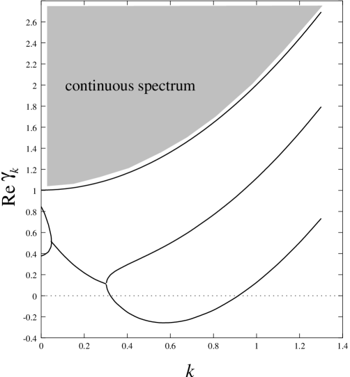
Figure 20: Damping decrement ${\mathrm{R}e}~{}\gamma_{k}$ for the static one-dimensional AS obtained from the numerical solution of Eq. (5.14) for different modes at $A=1.2$.

For $k>0.29$ Eq. (5.14) has two localized solutions and a continuous spectrum of $\gamma_{k}$ for $A=1.2$, all having ${\mathrm{R}e}~{}\omega(k)=0$. The curve at the bottom of the figure corresponds to $\delta\theta_{0}$, the curve in the middle to $\delta\theta_{2}$, and the curve on the top is the bottom of the continuous spectrum. From Fig. 20 one can see that the AS is unstable with respect to $\delta\theta_{0}$ (the corrugation instability) for a range of wave vectors $k\sim 1$. The analysis of $\gamma_{k}$ for different values of $A$ shows that the static one-dimensional spike AS in higher dimensions is unstable with respect to corrugation for all values of $A$ at which it exists.

When $0.05<k<0.29$, the complex frequency $\omega(k)$ for the modes $\delta\theta_{0,2}$ acquires a real part for $A=1.2$. The corresponding eigenfunctions for these modes, as well as $\gamma_{k}$, are complex-conjugate. For yet smaller values of $k$ the real part of $\omega$ vanishes once again, so we have two distinct solutions. The latter is related to the presence of two distinct solutions in the case of the one-dimensional AS studied in Sec. 5.1.2, which is obtained from Eq. (5.14) in the limit $k\rightarrow 0$. When the value of $A$ is decreased below $A=0.90$, these two distinct solutions disappear and the solution with a nonzero real part of $\omega(k)$ goes all the way to $k=0$.

Note that in the case $A_{b}\lesssim A\ll 1$ it can be easily shown that the AS is unstable with respect to the corrugation instability. Indeed, for $A\ll 1$ and $k\gg A^{2}$ the operator in right-hand side of Eq. (5.14) can be considered as a perturbation. Therefore, in the zeroth approximation we will have $\delta\theta_{0}=\delta\theta_{0}^{(0)}$, where $\delta\theta_{0}^{(0)}$ is given by Eq. (5.7). Then, in the first order of the perturbation theory we will have

$$\gamma_{k}=\left(-{5\over 4}+{75\pi^{2}A^{2}\over 2048k}+k^{2}\right)\left(1+{75\pi^{2}A^{2}\over 2048k}\right)^{-1},$$ (5.15)

which is negative for $k\lesssim 1$. Notice that according to this equation the fastest growing mode has $k\simeq 0.60$, what coincides with very good accuracy with the results of the numerical solution of Eq. (5.14) (see Fig. 20). Similarly, for $A_{b}\ll A\ll 1$ and $\alpha\ll\alpha_{\omega}$ it is easy to show that the AS will be unstable. Here we can also treat the right-hand side of Eq. (5.11) as a perturbation, so once again $\delta\theta_{0}=\delta\theta_{0}^{(0)}$. The solution of Eq. (5.11) in the first order of the perturbation theory with $\alpha/\epsilon^{2}\ll A^{4}$ and the exponential set to 1 then gives us $\gamma\simeq-\frac{5}{4}+{27\pi^{2}\sqrt{5}\over 1024}A^{2}\alpha^{1/2}\epsilon^{-1}<0$. Notice that by equating this expression to zero, one gets the value of $\alpha_{\omega}$ which differs from the one in Eq. (5.12) by only 10%.

5.1.5 Case $\alpha\gg 1$ and $k\not=0$: instability with respect to wriggling

Let us now turn to the mode $\delta\theta_{1}$. Since, because of the translational invariance Eq. (5.5) is identically satisfied for $k=0$ and $\gamma=0$ with $\delta\theta_{1}=d\bar{\theta}_{0}/dx$, it is of special interest to study its solutions for $|\gamma|\ll 1$ and $k\ll 1$. The small values of $k$ and $\gamma$ introduce a weak perturbation to the operators in Eq. (5.5) with $k=0$ and $\gamma=0$. Therefore, in the leading order of the perturbation theory we must take $\delta\theta_{1}=d\bar{\theta}_{0}/dx$, and in order to get $\gamma_{k}$ we must multiply Eq. (5.5) by the adjoint function $\delta\theta_{1}^{*}$ and integrate over $x$. As a result, in the first order in $\gamma_{k}$ and $k^{2}$ we obtain

$$-\gamma_{k}+k^{2}+\gamma_{k}\frac{A^{2}(1-\epsilon^{2}\alpha^{-1})}{2}\int_{-\infty}^{+\infty}\int_{-\infty}^{+\infty}\bar{\theta}_{0}^{2}(x)\delta\theta_{1}^{*}(x)|x-x^{\prime}|\delta\theta_{1}(x^{\prime})dxdx^{\prime}$$

$$\quad={\epsilon A^{2}\over 8\alpha}(\gamma_{k}-\alpha\epsilon^{-2}k^{2})\int_{-\infty}^{+\infty}\int_{-\infty}^{+\infty}\bar{\theta}_{0}^{2}(x)\delta\theta_{1}^{*}(x)(x-x^{\prime})^{2}\delta\theta_{1}(x^{\prime})dxdx^{\prime},$$ (5.16)

where we expanded the exponential in Eq. (5.5) up to the second order in $\epsilon$ and used the normalization $\int_{-\infty}^{+\infty}\delta\theta_{1}^{*}\delta\theta_{1}dx=1$. Recalling that $\delta\theta_{1}=d\bar{\theta}_{0}/dx$, we can calculate the integral in the right-hand side of Eq. (5.16). Using the symmetry properties of $\delta\theta_{1}$, we find this integral to be $2\int_{-\infty}^{+\infty}x\bar{\theta}_{0}^{2}\delta\theta_{1}^{*}dx\int_{-\infty}^{+\infty}\bar{\theta}_{0}dx<0$, since for $x<0$ we have $\delta\theta_{1}^{*}>0$ and vice versa. By a similar integration, one can show that the integral in the left-hand side of Eq. (5.16) is also negative. Then, it is easy to see that when $\alpha\gtrsim\epsilon$ (otherwise the AS would be unstable in one-dimension, see Sec. 5.1.6), for small values of $k$ we will have $\gamma_{k}\sim-\epsilon^{-1}A^{2}k^{2}<0$, so the one-dimensional static spike AS is in fact always unstable with respect to the $\delta\theta_{1}$ mode with small $k$ for $A\gg A_{b}$. These fluctuations should lead to wriggling of the AS. Moreover, it is possible to show that the static spike AS which is stable in one dimension is in fact unstable with respect to wriggling for all values of $A>A_{b}$. Indeed, for $A\sim A_{b}$ the operator in the right-hand side of Eq. (5.5), which is the only non self-adjoint operator there, can be considered as a perturbation, so we can assume that $\delta\theta_{1}=\delta\theta_{1}^{*}=\delta\theta_{1}^{(0)}$ and take $\bar{\theta}_{0}$ to be given by Eq. (3.3). Substituting this into Eq. (5.16), we obtain that for small values of $k$ the damping decrement $\gamma_{k}$ of the fluctuations leading to wriggling is given by

$$\gamma_{k}\simeq k^{2}\left[1-{A^{2}\over A_{b}^{2}}\left(1+\sqrt{1-{A_{b}^{2}\over A^{2}}}~{}\right)^{2}~{}\right].$$ (5.17)

From this equation one can see that $\gamma_{k}<0$, signifying an instability, for $A>A_{b}$ and sufficiently small $k$. Thus, in summary, the one-dimensional static spike AS is always unstable in higher dimensions, so the instabilities that are realized for sufficiently small $\alpha$ are meaningful only for the one-dimensional system.

5.1.6 Case $\alpha\ll 1$ and $k=0$: instability with respect to the onset of the traveling motion

In addition to the instability of the AS with respect to wriggling, another instability may be realized when $\alpha\ll 1$ [45]. As was already mentioned above, for $k=0$ Eq. (5.16) has a simple zero solution for any $\alpha$ due to the translational invariance. However, at some special value of $\alpha=\alpha_{T}$ the solution $\gamma=0$ may become doubly degenerate. This will happen when the coefficient in front of $\gamma$ in Eq. (5.16) vanishes. If this is the case, in addition to the trivial solution we will have another non-trivial zero solution, for which the value of $\gamma$ should change sign as the value of $\alpha$ passes through $\alpha_{T}$. This signifies an instability that leads to the onset of the traveling motion. It is not difficult to see that this instability will occur when $\alpha<\alpha_{T}\sim\epsilon$ for $A\lesssim 1$. In particular, when $A\ll 1$, we can put $\delta\theta_{1}^{*}=\delta\theta_{1}=\delta\theta_{1}^{(0)}$, since again the only non self-adjoint operator is the operator in the right-hand side of Eq. (5.5) and is small. After a little algebra, we obtain that the instability will occur at

$$\alpha_{T}=\left\{\begin{array}[]{lc}{\epsilon^{2}A^{2}\over A_{b}^{2}}\left[1+\sqrt{1-{A_{b}^{2}\over A^{2}}}~{}\right]^{2},&~{}~{}~{}A\sim A_{b},\\ \frac{1}{3}A^{2}\epsilon,&~{}~{}~{}A_{b}\ll A\ll 1.\end{array}\right.$$ (5.20)

Note that the last formula is in agreement with the results of Sec. 4.2.1. To analyze the dependence $\alpha_{T}(A)$ for $A\sim 1$ we solved for the conjugate function $\delta\theta_{1}^{*}$ numerically and then substituted it to Eq. (5.16). The resulting dependence $\alpha_{T}(A)$ is presented in Fig. 21.

Figure 21: Dependence $\alpha_{T}(A)$ for the static one-dimensional AS obtained from the numerical solution of Eq. (5.16).

Observe that for $A<1$ the value of $\alpha_{T}$ is given by Eq. (5.20) with an accuracy better than 10%.

5.1.7 Comparison of the pulsation and the traveling instabilities

According to Eqs. (5.12) and (5.20), for $A>1.58\epsilon^{1/6}$ we have $\alpha_{T}>\alpha_{\omega}$, so if one starts with the static spike AS at $A\sim 1$ and sufficiently large value of $\alpha$ and then gradually decreases $\alpha$, the AS will destabilize with respect to the fluctuation $\delta\theta_{1}$ and will transform into traveling. If, on the other hand, we have $A<1.58\epsilon^{1/6}$ at the start, the AS will destabilize with respect to the pulsations and will collapse after a few oscillations of its amplitude (see Sec. 6). Also, according to Eqs. (5.12) and (5.20), for $\alpha<\alpha_{c}=0.83\epsilon^{4/3}$ the one-dimensional static spike AS will be unstable regardless of the value of $A$, so we conclude that this AS can be excited only when $\alpha>\alpha_{c}$.

5.2 Stability of the three-dimensional radially-symmetric static spike autosoliton

So far we were studying the one-dimensional static spike AS in higher dimensions. Let us now turn to the radially-symmetric spike ASs. It turns out that up to the logarithmic terms, all the results on the stability of the two- and the three-dimensional radially-symmetric static spike ASs have the same dependence on $\epsilon$, so we will concentrate mostly on the three-dimensional AS. For the three-dimensional radially-symmetric static spike AS the small deviations $\delta\theta=\theta-\theta_{0}$ and $\delta\eta=\eta-\eta_{0}$ in the spherical coordinates can be taken as

$$\delta\theta=\e^{{\mathrm{i}}\omega t}Y_{nm}(\vartheta,\varphi)\delta\theta_{n\omega}(r),~{}~{}~{}\delta\eta=\e^{{\mathrm{i}}\omega t}Y_{nm}(\vartheta,\varphi)\delta\eta_{n\omega}(r),$$ (5.21)

where $Y_{nm}$ are the spherical harmonics. Then, Eqs. (2.15) and (2.16) linearized around $\theta_{0}$ and $\eta_{0}$ become

$$\left[-{d^{2}\over dr^{2}}-{2\over r}{d\over dr}+{n(n+1)\over r^{2}}+1+{\mathrm{i}}\omega-2\tilde{A}\tilde{\theta}_{0}\tilde{\eta}_{0}\right]\delta\theta_{n\omega} = \epsilon^{-1}\tilde{A}\tilde{\theta}_{0}^{2}\delta\eta_{n\omega},$$ (5.22)

$$\left[-{d^{2}\over dr^{2}}-{2\over r}{d\over dr}+{n(n+1)\over r^{2}}+\epsilon^{2}+{\mathrm{i}}\epsilon^{2}\alpha^{-1}\omega\right]\delta\eta_{n\omega}$$ (5.23)

$$=-\epsilon\tilde{A}^{-1}\left[-{d^{2}\over dr^{2}}-{2\over r}{d\over dr}+{n(n+1)\over r^{2}}+1+{\mathrm{i}}\omega\right]\delta\theta_{n\omega},$$

where, once again, length and time are measured in the units of $l$ and $\tau_{\theta}$, respectively, and we used the scaled variables given by Eq. (3.26). Equation (5.23) can be solved by means of the Green’s function, which in the case of the operator in the left-hand side of Eq. (5.23) multiplied by $r^{2}$ is (similar Green’s function was used in [21, 22])

$$G_{n\omega}(r,r^{\prime})=\left\{\begin{array}[]{ll}{I_{n+1/2}(\epsilon r\sqrt{1+{\mathrm{i}}\alpha^{-1}\omega})K_{n+1/2}(\epsilon r^{\prime}\sqrt{1+{\mathrm{i}}\alpha^{-1}\omega})\over\sqrt{rr^{\prime}}},&~{}~{}~{}r\leq r^{\prime},\\ {I_{n+1/2}(\epsilon r^{\prime}\sqrt{1+{\mathrm{i}}\alpha^{-1}\omega})K_{n+1/2}(\epsilon r\sqrt{1+{\mathrm{i}}\alpha^{-1}\omega})\over\sqrt{rr^{\prime}}},&~{}~{}~{}r\geq r^{\prime},\end{array}\right.$$ (5.26)

where $I_{n+1/2}(x)$ and $K_{n+1/2}(x)$ are the modified Bessel functions. Solving Eq. (5.23) with the use of Eq. (5.26), we obtain

$$\delta\eta_{n\omega}=-\epsilon\tilde{A}^{-1}\delta\theta_{n\omega}-\epsilon\tilde{A}^{-1}(1+{\mathrm{i}}\omega-{\mathrm{i}}\epsilon^{2}\alpha^{-1}\omega)\int_{0}^{\infty}G_{n\omega}(r,r^{\prime})\delta\theta_{n\omega}(r^{\prime})r^{\prime 2}dr^{\prime}.$$

Substituting this expression into Eq. (5.22), we obtain the following equation

$$\left[-{d^{2}\over dr^{2}}-{2\over r}{d\over dr}+{n(n+1)\over r^{2}}+1+{\mathrm{i}}\omega-2\tilde{A}\tilde{\theta}_{0}\tilde{\eta}_{0}+\tilde{\theta}_{0}^{2}\right]\delta\theta_{n\omega}$$ (5.28)

$$=-\tilde{\theta}_{0}^{2}(1+{\mathrm{i}}\omega-{\mathrm{i}}\epsilon^{2}\alpha^{-1}\omega)\int_{0}^{\infty}G_{n\omega}(r,r^{\prime})\delta\theta_{n\omega}(r^{\prime})r^{\prime 2}dr^{\prime}.$$

This equation determines the complex frequencies of different fluctuations as the functions of the control parameters and has to be solved as an eigenvalue problem. The instability of the AS will occur when ${\mathrm{R}e}~{}\gamma<0$, with $\gamma=-{\mathrm{i}}\omega$.

5.2.1 Case $\alpha\gg\epsilon^{2}$: instability with respect to the non radially-symmetric fluctuations

Let us first look at Eq. (5.28) at $\alpha\gg\epsilon^{2}$. In this case the terms proportional to $\alpha^{-1}$ in the right-hand side of Eq. (5.28) can be neglected, so the Green’s function $G_{n\omega}$ can be expanded in $\epsilon$. Then Eq. (5.28) becomes asymptotically

$$\left[-{d^{2}\over dr^{2}}-{2\over r}{d\over dr}+{n(n+1)\over r^{2}}+1-\gamma_{n}-2\tilde{A}\tilde{\theta}_{0}\tilde{\eta}_{0}+\tilde{\theta}_{0}^{2}\right] \delta\theta_{n}$$ (5.29)

$$=-{\tilde{\theta}_{0}^{2}(r)(1-\gamma_{n})\over 2n+1}\int_{0}^{\infty}g_{n}(r,r^{\prime})\delta\theta_{n}(r^{\prime})r^{\prime}dr^{\prime},$$

where

$$g_{n}(r,r^{\prime})=\left\{\begin{array}[]{ll}(r/r^{\prime})^{n},&r\leq r^{\prime},\\ (r^{\prime}/r)^{n+1},&r\geq r^{\prime}.\end{array}\right.$$ (5.32)

The operator in the left-hand side of Eq. (5.29) is a Schrödinger type operator with the attractive potential $-2A\tilde{\theta}_{0}\tilde{\eta}_{0}$, repulsive potential $\tilde{\theta}_{0}^{2}$ and the centrifugal potential $n(n+1)/r^{2}$.

As in the case of the one-dimensional AS, the modes $\delta\theta_{n}$ that can lead to instabilities are localized. From the translational symmetry of the problem we know that there is a localized solution $\delta\theta_{1}=d\tilde{\theta}_{0}/dr$ for $n=1$ which corresponds to $\gamma=0$. It is clear that since the potential in the left-hand side of Eq. (5.29) is able to localize a state at $n=1$ in the presence of the centrifugal potential, it will also be able to localize a state at $n=0$ in its absence. According to Sec. 3.2, we should in fact have an instability at the point $\tilde{A}=\tilde{A}_{b}=5.8$ where the solution in the form of the static three-dimensional radially-symmetric AS disappears. Also, it is natural to expect that the operator in the left-hand side of Eq. (5.29) will also be able to have a bound state for sufficiently small $n$ and sufficiently large $\tilde{A}$, when the role of the centrifugal potential decreases (see below). These will be the dangerous modes that we need to consider.

It is not difficult to show that for $\tilde{A}\gg 1$ the AS will be unstable with respect to the fluctuations with $n\not=0$. Indeed, according to the results of Sec. 3.2, for these values of $\tilde{A}$ the AS has the form of an annulus of large radius $R\sim\tilde{A}^{2}$ [see Eq. (3.44)]. According to Eqs. (3.38) and (3.42), the leading contribution to the potential in the left-hand side of Eq. (5.29) is $V(r)\cong-3\cosh^{-2}\left({r-R\over 2}\right)$. For $R\gg 1$ and $1\ll n\ll R$ all the other terms can be considered as a perturbation to the Schrödinger operator with this potential, so in the first order of the perturbation theory $\delta\theta_{0}=\delta\theta_{0}^{(0)}(r-R)$, where $\delta\theta_{0}^{(0)}$ is given by Eq. (5.7). In the first order of the perturbation theory we obtain

$$\gamma_{n}\simeq\left(-\frac{5}{4}+{n^{2}\over R^{2}}+{225\pi^{2}\over 2048n}\right)\left(1+{225\pi^{2}\over 2048n}\right)^{-1}.$$ (5.33)

This equation shows that for $R\gg 1$ there is a range of values of $n$ for which $\gamma_{n}<0$. The fact that the annulus must be unstable with respect to the shape deformations is an obvious consequence of its quasi one-dimensional character (see Sec. 5.1.4).

The presence of the localized solution $\delta\theta_{n}$ of Eq. (5.29) with $\gamma_{n}=0$ for $n>0$ signifies an instability of the radially-symmetric static AS with respect to the non radially-symmetric fluctuations resulting in the distortions of the spike and leading to its splitting (see Sec. 7). It is clear that this instability will occur easier at smaller values of $n$, so we have to solve Eq. (5.29) for $n=2$ (the case $n=1$ corresponds to the translation of the AS as a whole without any deformation). The numerical solution of Eq. (5.29) shows that the AS indeed becomes unstable with respect to the fluctuation with $n=2$ when $\tilde{A}>\tilde{A}_{c2}=8.4$. In general, the numerical solution of Eq. (5.29) shows that the static radially-symmetric spike AS is stable only in the narrow range $\tilde{A}_{b}<\tilde{A}<\tilde{A}_{c2}$. It is interesting to note that Eq. (5.33) with $n=2$, together with Eq. (3.44), gives the correct value of $A_{c2}$ with accuracy better than $5\%$.

When the value of $\tilde{A}$ is increased beyond $A_{c2}$, the buildup of the instability with $n=2$ will result in the splitting of the AS. After such a splitting event, the two newborn ASs will go apart until they are separated by a sufficiently large distance, and then will split again. Thus, the considered instability will result in self-replication of ASs (see Sec. 7). We would like to emphasize that the character of the instability that leads to self-replication in three-dimensional (and two-dimensional) systems is significantly different from that in one dimension. In the former the instability results in the buildup of the shape distortion that eventually leads to splitting, while in the latter the instability leads to the widening of the activator distribution profile and local breakdown in the AS center (see Sec. 6). Thus, self-replication of the AS in one dimension is qualitatively different from that in higher dimensions.

5.2.2 Case $\alpha\lesssim\epsilon^{2}$: instability with respect to the pulsations and the onset of the traveling motion

According to the general qualitative theory of ASs, when $\alpha$ becomes small, the AS may become unstable with respect to the pulsations with ${\mathrm{R}e}~{}\omega\not=0$. The analysis of Eq. (5.28) with $n=0$ shows that this instability may be realized only when $\alpha\sim\epsilon^{2}$ and ${\mathrm{R}e}~{}\omega=\omega_{0}\sim 1$. In view of this fact, we can drop 1 in the square roots in Eq. (5.26). Equation (5.28) can then be solved numerically. The results of this numerical solution are presented in Fig. 22.

Figure 22: (a) Stability diagram for the three-dimensional radially-symmetric AS. (b) Frequency $\omega_{0}$ at the threshold of the pulsation instability. Results of the numerical solution of Eq. (5.28). In (a) the upper solid line shows the values of $\alpha_{\omega}/\epsilon^{2}$ corresponding to the onset of the pulsation instability ($n=0$) , the lower solid curve shows the values of $\alpha_{T}/\epsilon^{2}$ corresponding to the instability leading to the onset of the traveling motion ($n=1$). The dotted lines correspond to the instabilities of the static AS at $\tilde{A}=\tilde{A}_{b}$ and $\tilde{A}=\tilde{A}_{c2}$.

The upper curve in Fig. 22(a) shows the critical values of $\alpha_{\omega}$ for the onset of this instability for those values of $\tilde{A}$ at which the AS is stable at $\alpha\gg\epsilon^{2}$. Figure 22(b) shows the frequency $\omega_{0}$ of the fluctuations at the threshold of the instability. From Fig. 22(a) one can see that the static three-dimensional AS is unstable for all values of $\tilde{A}$ if $\alpha<\alpha_{c}\simeq 3.7\epsilon^{2}$.

As was already noted, in addition to the modes studied above, we always have a dangerous mode $\delta\theta=d\tilde{\theta}/dr$ with $n=1$. The analysis of Eq. (5.28) shows that in addition to the trivial solution, at some $\alpha=\alpha_{T}\sim\epsilon^{2}$ this equation can have another solution with ${\mathrm{R}e}~{}\gamma=0$. As in the case of the one-dimensional AS, this solution will signify the instability which results in the AS starting to move as a whole. To find this instability point, we need to know the behavior of the Green’s function $G_{1\omega}(r,r^{\prime})$ at small values of ${\mathrm{i}}\omega$. Expanding the Bessel functions in Eq. (5.26) and finding the adjoint function $\delta\theta_{1}^{*}$ numerically, we calculate the coefficient in front of ${\mathrm{i}}\omega$ in the first order of the perturbation theory, keeping only the leading terms in $\epsilon$. The above mentioned instability will be realized when this coefficient vanishes. The lower solid line in Fig. 22(a) shows the values of $\alpha_{T}/\epsilon^{2}$ at which this happens. One can see that this instability occurs when the AS is already unstable with respect to the pulsations. Note that the numerical solution of Eq. (5.28) shows that the instabilities with respect to the fluctuations with $n\geq 2$ always happen for significantly lower values of $\alpha$.

5.3 Stability of the two-dimensional radially-symmetric static spike autosoliton

Finally, we will briefly discuss the stability of the two-dimensional static spike AS in the limit $\epsilon\rightarrow 0$. In the cylindrical coordinates $r,\varphi$ the small deviations $\delta\theta=\theta-\theta_{0}$ and $\delta\eta=\eta-\eta_{0}$ can be taken as

$$\delta\theta=\delta\theta_{n\omega}(r)\e^{{\mathrm{i}}\omega t-{\mathrm{i}}n\varphi},~{}~{}~{}\delta\eta=\delta\eta_{n\omega}(r)\e^{{\mathrm{i}}\omega t-{\mathrm{i}}n\varphi},$$ (5.34)

where $n$ is an integer.

The equation for $\delta\theta_{n\omega}$ is obtained by linearizing Eqs. (2.15) and (2.16) around $\theta_{0}$ and $\eta_{0}$ and eliminating $\delta\eta_{n\omega}$ by inverting the equation for $\delta\eta_{n\omega}$. As a result, using the scaled $\tilde{\theta}_{0}$ and $\tilde{\eta}_{0}$ given by Eq. (3.49), we arrive at the following equation for $\delta\theta_{n\omega}$

$$\left[-{d^{2}\over dr^{2}}-{1\over r}{d\over dr}+{n^{2}\over r^{2}}+1+{\mathrm{i}}\omega-2\tilde{A}\tilde{\theta}_{0}\tilde{\eta}_{0}+\tilde{\theta}_{0}^{2}\right]\delta\theta_{n\omega}$$ (5.35)

$$=-\tilde{\theta}_{0}^{2}(1+{\mathrm{i}}\omega-{\mathrm{i}}\epsilon^{2}\alpha^{-1}\omega)\int_{0}^{\infty}G_{n\omega}(r,r^{\prime})\delta\theta_{n\omega}(r^{\prime})r^{\prime}dr^{\prime},$$

where $G_{n}(r,r^{\prime})$ is given by

$$G_{n}(r,r^{\prime})=\left\{\begin{array}[]{ll}I_{n}(\epsilon r\sqrt{1+{\mathrm{i}}\alpha^{-1}\omega})K_{n}(\epsilon r^{\prime}\sqrt{1+i\alpha^{-1}\omega}),&~{}~{}~{}r<r^{\prime},\\ I_{n}(\epsilon r^{\prime}\sqrt{1+{\mathrm{i}}\alpha^{-1}\omega})K_{n}(\epsilon r\sqrt{1+{\mathrm{i}}\alpha^{-1}\omega}),&~{}~{}~{}r>r^{\prime},\end{array}\right.$$ (5.38)

where $I_{n}$ and $K_{n}$ are the modified Bessel functions. The analysis of this equation can be performed in the way completely analogous to that of Eq. (5.28). It is clear that the instabilities of the two-dimensional static spike AS will be qualitatively the same as those of the three-dimensional AS. We would like to emphasize that as in the case of the three-dimensional AS, splitting and self-replication of the static spike AS in the two-dimensional system is related to the buildup of the fluctuation with $n=2$ describing a non-symmetric distortion of the AS. Because of the very slow convergence of the asymptotic theory in two dimensions (recall that the small parameter here is $1/\ln\epsilon^{-1}$) we will not present a detailed study of Eq. (5.35).

6 Pattern formation scenarios in one dimension

In the following two Sections we present the results of the numerical simulations of the Gray-Scott model for sufficiently small $\epsilon$ and $\alpha$ and compare them with the results of our asymptotic analysis.

A word needs to be said about the numerical methods we used in various parts of the paper. Whenever it was not said otherwise, length and time were measured in the units of $L$ and $\tau_{\eta}$, respectively. To simulate the original reaction-diffusion equations we used a simple explicit second-order scheme both in one and two dimensions. We used neutral boundary conditions in all our simulations. In order to resolve the details of the shape of the spike, sufficiently small spatial discretization step was needed. It was found that the step $\Delta x=0.25l$ gave the solutions with accuracy of a few per cent. The stiffness of equations at small $\epsilon$ or $\alpha$ makes the simulations very time consuming, so two-dimensional simulations were done on the massively parallel supercomputer (SGI-Cray Origin 2000). A typical running time for the simulations shown in the paper is about 1 hour on 16 processors.

In addition to the direct simulations of the original reaction-diffusion equations, we used various methods in solving the equations obtained from the asymptotic procedures. In solving for the sharp distributions in the case of the static spike ASs we used relaxation methods with second-order discretization. In solving the nonlinear eigenvalue problems we used a combination of the relaxation method and iterative method. In the case of the traveling spike ASs we used shooting method to solve the obtained ODEs. In analyzing the stability of the static spike ASs we used second-order discretization of the linear operators in a sufficiently large finite domain and then diagonalized the obtained matrices. The solution of the ODEs and the diagonalization were performed using Mathematica 3.0. In all the cases the accuracy of the numerical solutions is better than a few per cent.

6.1 Properties of the static spike autosoliton

In Sec. 3.1 we found that the static spike ASs can form in the Gray-Scott model when $\epsilon\ll 1$. In one dimension these AS are stable when $\alpha>\alpha_{0}=0.33$ in the whole region of its existence $A_{b}<A<A_{d}$. Our numerical simulations of Eqs. (2.15) and (2.16) show that the value of $A_{b}$ is given by Eq. (3.6) with very good accuracy (less than 1%) already for $\epsilon<0.1$, while the value of $A_{d}$ approaches its asymptotic value $A_{d}=1.35$ for $\epsilon\lesssim 0.01$ and increases somewhat for larger $\epsilon$ (for example, for $\epsilon=0.05$ we found $A_{d}=1.48$). These results are robust against decreasing $\epsilon$ from 0.01 to 0.001 and smaller. For $A_{b}<A<1$ the distributions of $\theta$ and $\eta$ are described by Eqs. (3.3) and (3.7) with accuracy better than 10% for $\epsilon\lesssim 0.1$.

The numerical solution of Eqs. (2.15) and (2.16) for $\epsilon=0.05$ and $A=1.4$ in the form of the one-dimensional static spike AS is presented in Fig. 23.

Figure 23: (a) Distributions of $\theta$ and $\eta$ in a static spike one-dimensional AS; (b) Potential $V$ from Eq. (3.18). Results of the numerical solution of Eqs. (2.15) and (2.16) with $\epsilon=0.05$, $\alpha=1$, and $A=1.4$.

The shape of the distributions of $\theta$ and $\eta$ remains qualitatively the same all the way up to $A_{d}=1.48$, but when $A$ approaches $A_{d}$ the spike widens somewhat and its maximum becomes flatter. One can see that the potential $V$ from the nonlinear eigenvalue problem [see Eq. (3.18)] shown in Fig. 23(b) indeed assumes a complicated shape predicted by the asymptotic theory (Sec. 3). According to the asymptotic theory, the value of $\theta_{\mathrm{m}ax}$ should decrease with the increase of $A$ for $A>1.2$ (see Fig. 5), and at $A>A_{d}$ the solution in the form of a single spike should disappear. This can also be seen from the simulations of the one-dimensional Gray-Scott model with $\epsilon=0.05$ (Fig. 24).

Figure 24: Dependences $\theta_{\mathrm{m}ax}$ and $\eta_{\mathrm{m}in}$ in the one-dimensional static spike AS obtained from the numerical solution of Eqs. (2.15) and (2.16) with $\epsilon=0.05$.

Observe the similarity between Fig. 24 and Fig. 5 obtained from the asymptotic theory. Also observe that the values of $\theta_{\mathrm{m}ax}$ for $A>1$ are smaller for finite values of $\epsilon$ than those predicted by the asymptotic theory. When the value of $A$ becomes greater than $A_{d}$, a dip in the distribution of $\theta$ appears in the center of the spike followed by a rapid decrease of the value of $\theta$ there (local breakdown) resulting in the AS splitting into two spikes. These spikes go away from each other and then split again, until the system becomes filled with a periodic pattern of spikes. This process of self-replication of the static spike ASs in the Gray-Scott model was studied in detail in [50, 55].

From the physical point of view, the existence of the static AS in which for $\epsilon=l/L\ll 1$ the distribution of $\theta=X/X_{0}$ has the form of a spike [see Fig. 23(a)] is determined by the diffusion processes and the special features of the autocatalytic reaction in Eq. (2.1) (see Sec. 2). Due to this reaction, the self-production of substance $X$ occurs accompanied by the decrease of the amount of substance $Y$. The rate of this reaction is $R\sim X^{2}Y$, so seemingly the concentration of substance $Y$ should rapidly decrease. This, however, does not occur, and the high rate of the reaction in the spike is maintained by the strong diffusion influx of substance $Y$ from the neighboring regions of size of order $L$. This ensures a finite concentration of substance $Y$ in the spike which is necessary to maintain a high rate of the self-production of substance $X$. The diffusion current of substance $Y$ is roughly $Y_{0}/L$, that is, it increases with $A\sim Y_{0}$ [see Eq. (2.10)], but the reaction rate $R$ grows as $X^{2}Y$, so due to the increase of $R$ with the increase of $X\sim A\sim Y_{0}$ the concentration of $Y\sim A^{-2}\sim Y_{0}^{-2}$ [see Eqs. (3.5)] decreases faster in the spike as the value of $Y_{0}$ is increased. Therefore, for large enough $Y_{0}$ the diffusion current cannot maintain high reaction rate in the spike. This explains why for large enough $A\sim Y_{0}$ the value of $\theta\sim X$ starts decreasing with the increase of $A$ and at some $A=A_{d}$ the solution in the form of the static spike AS disappears.

6.2 Formation and collapse of the pulsating autosoliton

In Sec. 5 we found that for $\alpha<0.33$ the static spike AS in the one-dimensional Gray-Scott model may become unstable with respect to the pulsations, with the critical value of $\alpha$ rapidly decreasing with the increase of $A$ [see Eq. (5.12)]. Our numerical simulations showed that in a sufficiently large system this instability leads to the growth of self-oscillations of the AS amplitude. In other words, this instability leads to the transformation of the static AS into pulsating [9, 10, 11]. Figure 25 presents the results of the simulation of such a process for $\epsilon=0.05$, $\alpha=0.024$, and $A=1.2$.

Figure 25: Dependences $\theta_{\mathrm{m}ax}(t)$ and $\eta_{\mathrm{m}in}(t)$ for the static spike AS at the onset of the pulsations. Results of the numerical solution of Eqs. (2.15) and (2.16) for $\epsilon=0.05$, $\alpha=0.024$ and $A=1.2$

The value of $\alpha_{\omega}=0.0255$ found in the simulations for these parameters agrees with the results of Sec. 5 with accuracy better than 5% (see Fig. 19). Also, the critical frequency agrees with the results of Sec. 5 within 1%. Note that for these values of $A$ the value of $\alpha_{\omega}$ given by Eq. (5.12) (which is also predicted in [51]) turns out to be off by a factor of 4. According to the results of the simulations, the pulsating AS seems to be unstable for all values of the parameters. After a few oscillations of its amplitude, it collapses into the homogeneous state (Fig. 25).

6.3 Properties of the traveling spike autosolitons

The condition $\alpha\ll 1$ means that the inhibitor $Y$ is much slower than the activator $X$. The appearance of pulsation instability is due to the fact that because of its sluggishness the inhibitor cannot control rapidly varying fluctuations of the activator. The lag in the inhibitor reaction also determines the existence of the traveling spike AS in the Gray-Scott model at $\alpha\ll 1$ and $\epsilon\gtrsim\alpha^{1/2}$. The supply of the substance $Y$ into the spike of the traveling AS which is necessary to maintain high reaction rate $R$ occurs by the AS running on the regions with high values of $Y$. The situation here resembles combustion process. The numerical simulations of Eqs. (2.15) and (2.16) in one dimension confirm the conclusions of Sec. 4 about the existence of the traveling spike ASs. Figure 26(a) shows the distributions of $\theta$ and $\eta$ in the form of an ultrafast traveling spike AS for $\epsilon=\infty$, $\alpha=0.05$, and $A=2$.

Figure 26: Two types of traveling spike AS: case $\epsilon\gg\alpha^{1/2}$ (a) and $\epsilon\sim\alpha$ (b). Results of the numerical solution of Eqs. (2.8) and (2.9). In (a) $L=0$, $\alpha=0.05$, $A=2$, length is measured in the units of $l$. In (b) $\epsilon=0.05$, $\alpha=0.05$, $A=1.2$, length is measured in the units of $L$.

The speed of this AS was found to be $c=7.3$, which agrees within 5% with that of Eq. (4.7). Also, the shape of the traveling spike AS is in agreement with the predictions of Sec. 4.1.

When the value of $\epsilon$ becomes smaller, or, more precisely, the value of $L$ becomes sufficiently large, the concentration of substance $Y$ in the front of the traveling spike decreases due to diffusion, so the speed of the AS decreases. This explains the possibility of the existence of two types of the traveling spike ASs studied in Sec. 4: the ultrafast traveling spike AS, which forms at $\epsilon\gtrsim\alpha^{1/2}$, and the slower traveling spike AS, which forms at $\epsilon^{2}\lesssim\alpha\lesssim\epsilon$. The numerical simulations confirm this statement. Figure 26(b) shows the distributions of $\theta$ and $\eta$ in the form of a slower traveling spike AS obtained from the numerical solution of Eqs. (2.15) and (2.16) for $\epsilon=0.05$, $\alpha=0.05$ and $A=2$. The speed of this AS was found to be $c=1.26$, much smaller than the speed of the ultrafast traveling AS discussed in the preceding paragraph. The shape of the slower traveling spike AS agrees with that found in the asymptotic theory (see Sec. 4.2). Figure 27 shows the dependence of the AS speed $c$ on $A$ at different values of $\alpha$ obtained from the numerical solution of Eqs. (2.15) and (2.16) with $\epsilon=0.05$.

Figure 27: Dependences $c(A)$ for the traveling spike AS at different values of $\alpha$ obtained from the numerical solution of Eqs. (2.15) and (2.16) with $\epsilon=0.05$.

Note that the curves $c(A)$ in Fig. 27 terminate at sufficiently large values of $A$. This is due to the fact that when the value of $A$ exceeds a certain critical value which depends on $\alpha$, the traveling AS starts splitting as it moves. This is in agreement with the predictions of Sec. 4.2.3 about the disappearance of the solution in the form of the traveling AS due to the onset of the oscillations in the back of the spike for sufficiently large values of $A$.

Two ultrafast traveling ASs moving towards each other annihilate, what follows from the physics of their existence. A much more diverse situation is realized in the case $\epsilon^{2}\lesssim\alpha\lesssim\epsilon$ when the slower traveling spike AS exist. Here the ASs moving towards each other can annihilate before colliding or bounce off each other and start traveling in the opposite direction as a result of the interaction via the diffusion of the inhibitor (a diffusion precursor). Also, as was shown in Sec. 5.1.7, when $A>1.58\epsilon^{1/6}$, the static spike AS may spontaneously transform into traveling when the value of $\alpha$ is decreased. This phenomenon was studied by Osipov and Severtsev in [45] in a simplified version of the Gray-Scott model and is observed in our simulations of Eqs. (2.15) and (2.16) as well. Comparing Fig. 27 with Fig. 24, one can see that there exists a parameter region where it is possible to excite both the static and the traveling ASs simultaneously.

According to Fig. 27, when the value of $A$ becomes sufficiently close to $A_{d}$, the speed of the traveling spike AS may go to zero for a range of $\alpha$. When $\epsilon=0.05$, this happens when $0.03<\alpha<0.06$. According to the simulations, at $\epsilon=0.05$ and $A=1.34$ the bifurcation of the static and the traveling ASs changes from subcritical to supercritical, so at higher values of $A$ their coexistence is no longer possible.

In our numerical simulations we also found the phenomenon of self-replication of the traveling spike ASs at large enough values of $A$. This phenomenon is illustrated in Fig. 28 which shows the density plots of the distributions of $\theta$ and $\eta$ as functions of $x$ (horizontal axis) and $t$ (vertical axis) for $\epsilon=0.05$, $A=2$, and several values of $\alpha$.

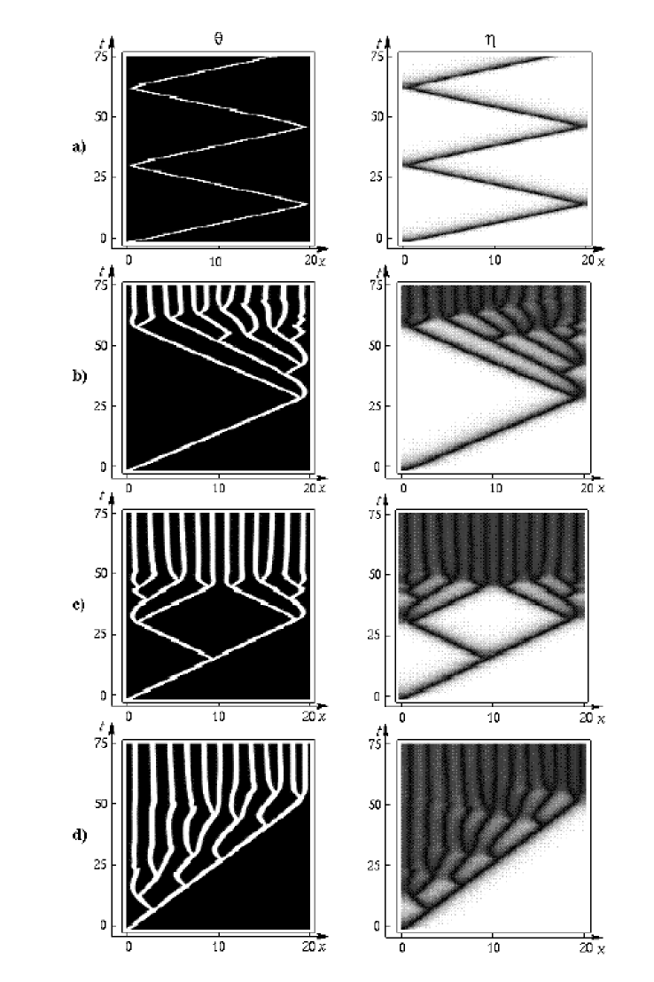
Figure 28: Self-replication of the traveling spike AS. Results of the numerical solution of Eqs. (2.15) and (2.16) with $\epsilon=0.05$, $A=2$; $\alpha=0.05$ (a), $\alpha=0.07$ (b), $\alpha=0.075$ (c), $\alpha=0.1$ (d). Darker areas correspond to lower values of $\theta$ and $\eta$.

One can see that for $\alpha=0.05$ the traveling AS goes back and forth between the system boundaries bouncing elastically off of them. When the value of $\alpha$ is increased to $\alpha=0.07$, a collision with the boundary stimulates a splitting event, which is followed by consecutive splitting of the newborn traveling spikes. Eventually, the system becomes filled with a stationary periodic pattern of spikes. Note that this pattern is stable in spite of the small value of $\alpha$ and the large value of $A$ at which the solution in the form of the static spike AS does not exist. When the value of $\alpha$ is increased to $\alpha=0.075$, the traveling AS starts splitting as it moves, and when $\alpha=0.1$, splitting occurs more frequently. Observe that a small increase in the value of $\alpha$ leads to a significant decrease of the distance between the consecutive splitting events. Also, observe that despite splitting, the speed of the leading traveling spike remains practically constant. This is in agreement with the results of Sec. 4.2.3 which attribute the splitting to the onset of the oscillatory behavior in the tail of the traveling spike AS. The behavior of $\theta$ and $\eta$ in the back of the spike only weakly affects the front of the spike, whose shape determines the speed of the traveling spike AS for sufficiently small values of $\alpha$ and sufficiently large values of $A$ (see Sec. 4.2.2). Notice that self-replication of the traveling spike AS and wave reflection in the Gray-Scott model was first observed numerically in [56].

The results on the existence of the static and the traveling ASs, and the stability of the static AS in one dimension obtained in the previous sections, together with the results of the numerical simulations, are summarized in Fig. 29.

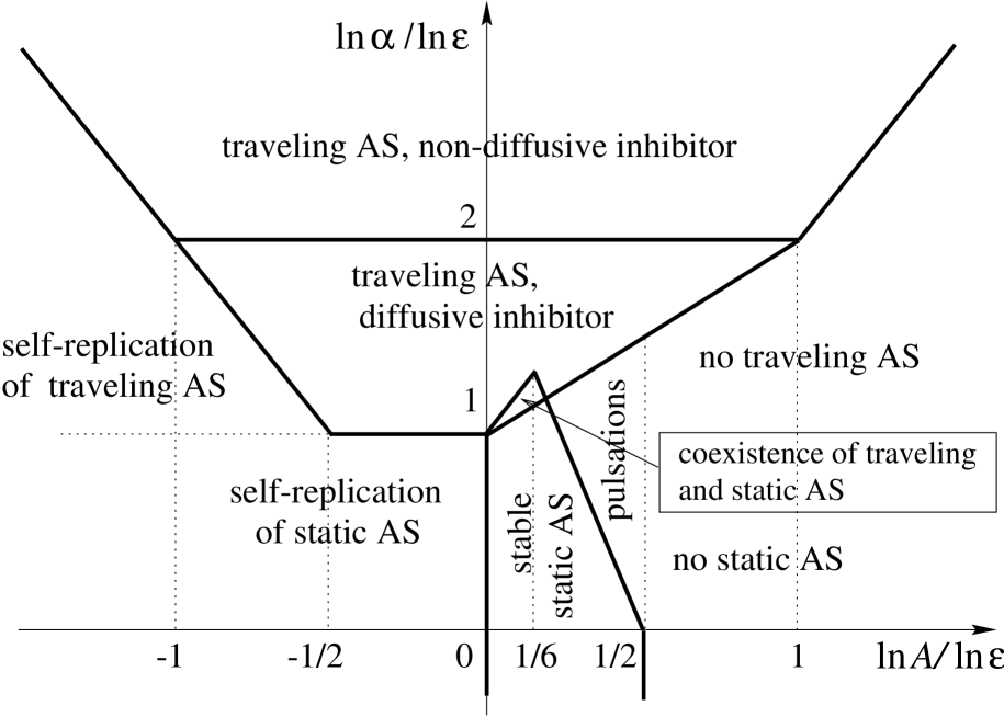
Figure 29: Diagram of the existence and the stability of different ASs in one dimension in the limit $\epsilon\rightarrow 0$.

This figure shows the domains of existence and the instability lines for the ASs in the $\ln\alpha-\ln A$ plane in the limit $\epsilon\rightarrow 0$.

7 Pattern formations scenarios in two dimensions

Up to now, we studied the dynamics of the spike patterns in the one-dimensional Gray-Scott model. Now we are going to study the pattern formation scenarios in the two-dimensional Gray-Scott model.

7.1 Granulation of the one-dimensional static spike autosoliton

In Sec. 5.1.4 we showed that in two dimensions the static spike AS in the form of a stripe is unstable in the whole region of its existence $A_{b}<A<A_{d}$ with respect to the corrugation instability, that is, the fluctuation $\delta\theta_{0}$ with $k\simeq 0.6l^{-1}$, even for $\alpha>0.33$. The growth of such a short-wave fluctuation should lead to the granulation of the stripe into small spots of size of order $l$. It is obvious that any wriggled stripe will also granulate into small spots. Figure 30 shows such a process obtained from the simulations with $\epsilon=0.05$, $\alpha=0.5$ and $A=2$.

Figure 30: Granulation of a stripe. Results of the numerical solution of Eqs. (2.15) and (2.16) with $\epsilon=0.05$, $\alpha=0.5$, and $A=2$. The system is $2.5\times 2.5$. The shades of gray show the distribution of $\eta$. The spots show the regions where $\theta>10$.

One can see that the stripe indeed granulates to spots of size of order $l$ which then go away from each other until they become uniformly distributed across the system. Self-replication of spots may occur during this process (see below).

7.2 Properities of the radially-symmetric static spike autosoliton

As was shown in Sec. 3.3 and Sec. 5.3, static radially-symmetric AS in two dimensions exists in a relatively narrow range of the values of $A\sim\epsilon$. From our numerical simulations we see that at $\epsilon=0.05$ and sufficiently large values of $\alpha$ a localized stimulus applied to the system at $t=0$ evolves into a stable static radially-symmetric spike AS at $0.38<A<0.65$. When $\alpha$ becomes sufficiently small, this region becomes even narrower since the AS becomes unstable with respect to the pulsations at sufficiently small $A$. If this is the case, an initial stimulus may produce a state which is close to a radially-symmetric AS, which after several pulsations will collapse. The process here is similar to the onset of the pulsations of the one-dimensional AS shown in Fig. 25. When the value of $\alpha$ becomes smaller than some value $\alpha_{c}$, static radially-symmetric AS becomes unstable for all values of $A$ and can no longer be excited.

7.3 Self-replication of the static radially-symmetric autosoliton

As was shown in Sec. 5.2 and Sec. 5.3, when the value of $A$ becomes greater than some critical value $A_{c2}$, the radially-symmetric static spike AS looses stability with respect to the radially non-symmetric fluctuations. The growth of such fluctuations leads to splitting and self-replication of the AS. In our simulations we found that for $\epsilon=0.05$ and sufficiently large $\alpha$ static radially-symmetric spike AS becomes unstable and self-replicates at $A\geq 0.7$. Such a process for $\epsilon=0.05$, $\alpha=0.5$, and $A=2$ is shown in Fig. 31.

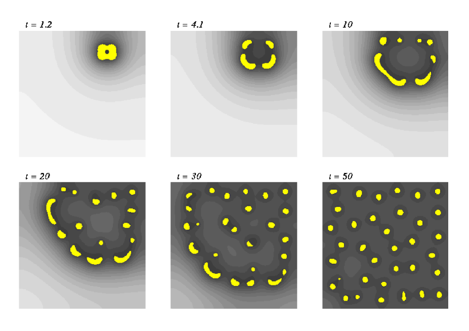
Figure 31: Self-replication of spots in two dimensions. Results of the numerical solution of Eqs. (2.15) and (2.16) with $\epsilon=0.05$, $\alpha=0.5$, and $A=2$. The system is $5\times 5$. The shades of gray show the distribution of $\eta$. The spots show the regions where $\theta>10$.

From this figure one can see that the initial condition in the form of a rectangle of size of a few $l$ splits into four (which is due to the rectangular shape of the initial condition and the fact that the value of $A$ is well above $A_{c2}$), and then the newborn spots go on splitting until the system gets filled with an irregular arrangement of spots, with the characteristic distance between the spots much less than $L$. We would like to emphasize that the patterns observed in our simulations are essentially different from the domain patterns that form in N-systems [20, 21, 22, 23, 24]. The distributions of the activator in our simulations consist of the small spots instead of the sharp interfaces, and in the spots they are close to those in the radially-symmetric static spike AS. This is illustrated in Fig. 32 which shows the distribution of $\theta$ at one of the moment of the simulation shown in Fig. 31.

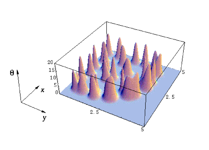
Figure 32: Distribution of $\theta$ in the simulation of Fig. 31 at $t=30$.

When the value of $\alpha$ becomes of order $\epsilon$, the dynamics of splitting significantly changes. Figure 33 shows the evolution of the system with $\epsilon=0.05$, $\alpha=0.1$, $A=3$, and a localized initial condition.

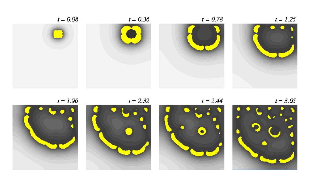
Figure 33: Splitting as a result of the formation and the breakdown of a quasi one-dimensional wave. Results of the numerical solution of Eqs. (2.15) and (2.16) with $\epsilon=0.05$, $\alpha=0.1$, and $A=3$. The system is $5\times 5$. The shades of gray show the distribution of $\eta$. The spots show the regions where $\theta>10$.

As was already mentioned in Sec. 6, a decrease in $\alpha$ means greater sluggishness of the inhibitor, so the pieces that form after splitting of an initial spot can go a greater distance apart and become more elongated than in Fig. 31 (where $\alpha\gg\epsilon$). The state that forms here is close to a torn-up quasi one-dimensional wave of width of order $l$. This is natural to expect since, as we showed in Sec. 4.2 and Sec. 6, the traveling spike ASs are realized in the system for these values of the parameters. In this case the formation of new spots occurs as a result of their pinching off of the tips of the quasi one-dimensional wave pieces, that is, they sort of drip off from them. This process is illustrated in Fig. 34 which shows the distribution of $\theta$ at one moment of the simulation in Fig. 33.

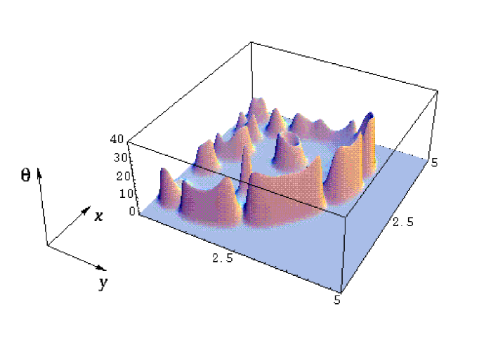
Figure 34: Distribution of $\theta$ in the simulation of Fig. 33 at $t=2.44$.

The spots that drip off from the wave pieces can further transform into quasi one-dimensional waves which in turn break up. As a result, the system becomes filled with a stable stationary pattern of spots, just as in the case of large $\alpha$ (see the last in Fig. 33).

7.4 Spatio-temporal chaos

For small enough values of $\alpha$ and $A$ we were able to observe spatio-temporal chaos. Figure 35 shows the development of a chaotic pattern at $\epsilon=0.1$, $\alpha=0.04$, and $A=1$.

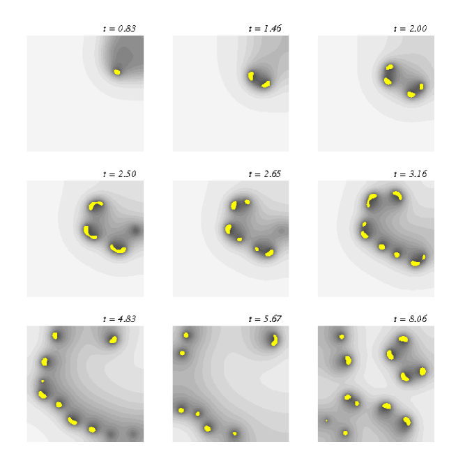
Figure 35: Formation of spatio-temporal chaos. Results of the numerical solution of Eqs. (2.15) and (2.16) with $\epsilon=0.1$, $\alpha=0.04$, and $A=1$. The system is $10\times 10$. The shades of gray show the distribution of $\eta$. The spots show the regions where $\theta>5$.

This pattern does not transform to a stationary pattern of spots even for very long simulation times ($t>100$). The stochastization of the pattern is caused by random splitting of spots and the disappearance of some of the spots due to their annihilation upon collision with the bigger spots. We would expect that these effects will be most pronounced at $\alpha\sim\epsilon^{2}$ and $A\sim A_{c2}$ when the static radially-symmetric AS is close to the instabilities with respect to the pulsations and the onset of the traveling motion (Fig. 22) and is unstable with respect to splitting. Notice that such chaotic patterns are also observed in semiconductor structures [12], combustion systems [14], and chemical systems [15].

7.5 Radially diverging waves

For larger values of $A$ and sufficiently small $\alpha$ an initially localized spot transforms into a circular stripe of growing radius (Fig. 36).

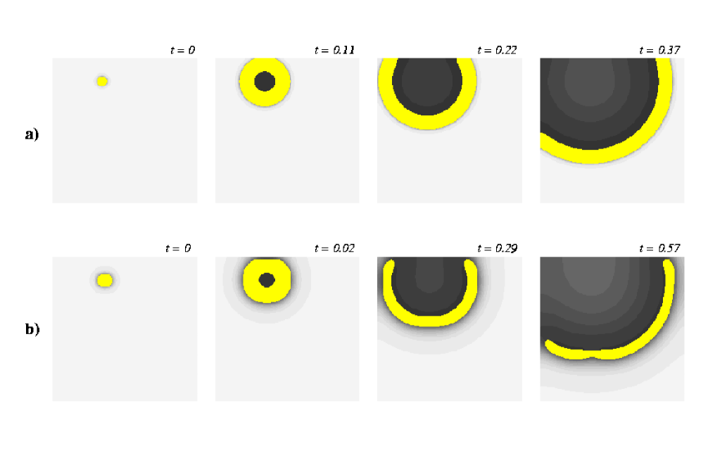
Figure 36: Propagation of waves in the Gray-Scott model. Results of the numerical solution of Eqs. (2.15) and (2.16) with (a) $\epsilon=0.2$, $\alpha=0.05$, and $A=1.5$; (b) $\epsilon=0.1$, $\alpha=0.05$, $A=1.5$. In (a) the system is $10\times 10$; in (b) the system is $5\times 5$. The shades of gray show the distribution of $\eta$. The spots show the regions where $\theta>10$.

When $\alpha$ is very small ($\alpha\lesssim\epsilon^{2}$), this wave does not tear up and disappears at the system boundary [Fig. 36(a)]. When, on the other hand, we have $\alpha\sim\epsilon$, the wave rebounds from the boundary and parts of it annihilate, so at some moment it tears up [Fig. 36(b)]. The tips of this wave get repelled from the boundary, so the wave propagates across the system until it annihilates upon collision with the boundary at its opposite side.

7.6 Spike spiral wave

As was shown in Sec. 4.1 and Sec. 6, the ultrafast traveling spike AS can form in one dimension when $\alpha\ll 1$ and $\epsilon=\infty$ (or $L=0$). In our numerical simulations we found that in two dimensions the solution in the form of the traveling stripe is stable in a wide range of $A$, so it is natural to expect that at the same parameters it is possible to excite a steadily rotating spiral wave. The formation of such a wave at $\alpha=0.1$ and $A=2$ is shown in Fig. 37.

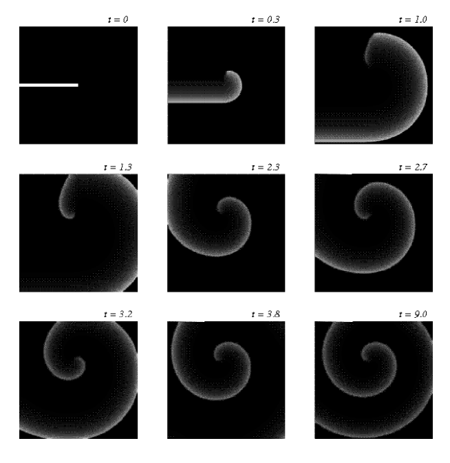
Figure 37: Formation of a steadily rotating spiral wave. Distribution of $\theta$ obtained from the numerical solution of Eqs. (2.8) and (2.9) with $L=0$, $\alpha=0.1$, and $A=2$. Length and time are measured in the units of $l$ and $\tau_{\theta}$, respectively. The system is $100\times 100$.

We would like to emphasize that this wave is essentially different from the spiral waves observed in N-systems in that in the cross-section it has a form of a narrow spike and does not have a front and a back separated by a large distance, as is the case in N-systems (see, for example, [2, 3, 5, 6, 7]). Note that the spiral wave shown in Fig. 37 is precisely the kind of the wave that is observed in the experiments on Belousov-Zhabotinsky reaction, and in the cardiac tissue, where such waves are thought to cause abnormal heart rhythms (see, for example, [3, 5] and references therein). Recently, we proposed an asymptotic theory of these spiral wave in the Gray-Scott model [57].

8 Discussion

While the work on this paper was being done, a number of publications on the Gray-Scott model appeared in the literature. The publications that are most relevant to our analysis are those of [50, 51].

In [51] Doelman et al. present an asymptotic study of the static AS and periodic strata in the one-dimensional Gray-Scott model. They perform a singular perturbation analysis of the localized and spatially periodic stationary solutions in a limited region of the parameter space. Their results are in agreement with ours in this parameter region. However, the conclusions of the authors may be somewhat confusing since they do not use the natural scaling of the Gray-Scott model given by Eqs. (2.15) and (2.16). Instead, they introduce such dimensionless quantities that the original Eqs. (2.3) and (2.4) become

$${\partial U\over\partial t} = {\partial^{2}U\over\partial x^{2}}-UV^{2}+\delta^{2}a(1-U),$$ (8.1)

$${\partial V\over\partial t} = \delta^{2}{\partial^{2}V\over\partial x^{2}}+UV^{2}-\delta^{\beta}bV,$$ (8.2)

where $U$ is the inhibitor, $V$ is the activator, $\delta$ is the small parameter, $a$ and $b$ are constants of order one, and $\beta$ ($=\frac{2\alpha}{3}$ from the first of [51]) is a parameter that lies in the interval from zero to one. The solutions are studied in the limit $\delta\rightarrow 0$.

It is clear that the scaling introduced in Eqs. (8.1) and (8.2) does not represent the true time and length scales of the problem, which are represented by Eqs. (2.15) and (2.16) of our paper. It is easy to see that Eqs. (8.1) and (8.2) can be reduced to Eqs. (2.15) and (2.16) with

$$\epsilon=\delta^{4-\beta\over 2}\sqrt{a\over b},~{}~{}~{}\alpha=\delta^{2-\beta}{a\over b},~{}~{}~{}A=\delta^{1-\beta}{\sqrt{a}\over b}.$$ (8.3)

Observe that the scaling in Eqs. (8.1) and (8.2) forces certain relations between the true parameters $\epsilon$, $\alpha$, and $A$, so in fact such a choice of scaling significantly restricts the parameter space studied by Doelman et al., leading them to incorrect conclusions about non-existence of certain types of solutions.

According to the results of the first paper in [51], the static one-dimensional AS exists only when $\beta\in[0,1)$ as $\delta\rightarrow 0$. This statement is based on the fact that the coefficient in front of the last term in the right-hand side of Eq. (8.1) scales as $\delta^{2}$. On the other hand, as we showed in Sec. 3.1, this AS in fact exists in a wider range of the parameters as long as $\epsilon\ll 1$, so in fact such a scaling is not a necessary condition for the AS existence. This fact was noticed by the authors in the more recent paper in [51].

The case $\beta=0$ is equivalent to $A\sim A_{b}$ in our notation. Our result that the solution exists only at $A>A_{b}=\sqrt{12\epsilon}$ is in agreement with the result of [51] that the solution exists at $a>144b^{3}$. Notice that the analogous method of finding $A_{b}$ for the ASs in systems of small size was introduced two decades ago by Kerner and Osipov [16]. There they performed an analysis of a very similar model — the Brusselator. The results obtained by them at $A\sim A_{b}$ for the Brusselator differ from those presented in our paper only by numerical coefficients. A calculation similar to that of Sec. 3.1.1 was performed by Dubitskii, Kerner, and Osipov for the Gierer-Meinhardt model [42] (see also [11]). Osipov and Severtsev also performed such an analysis for a simplified version of the Gray-Scott model, which are also very similar to the results of the first part of Sec. 3.1 [45]. The advantage of the method of Doelman et al., however, is that it rigorously shows the existence of the static spike AS for $A_{b}\lesssim A\ll 1$ and $\epsilon\ll 1$.

Doelman et al. claim that the solution obtained at $\beta=0$ is valid with accuracy to $\delta\sim\epsilon^{1/2}$. On the other hand, the analysis of Sec. 3.1 suggests that this solution is actually valid with a much better accuracy $\epsilon$. In fact, $\epsilon$ is the true small parameter of the problem, and the asymptotic procedure for obtaining the solutions for $\epsilon\ll 1$ can be constructed regardless of all other parameters of the problem with accuracy better than $\epsilon^{1/2}$ (see the discussion at the end of Sec. 3). Note that this procedure for general V- and $\Lambda$-systems was first introduced by Dubitskii, Kerner, and Osipov in [42] (see also [11]).

For $\beta>0$ Doelman et al. claim that the solution obtained by them is accurate to order $\delta^{1-\beta}$. They forget that although the accuracy with which the asymptotic equations describe the actual distribution of $V$ increases as $\beta$ decreases, the accuracy of the matching condition, namely, the fact that the true $U(0)$ is non-zero, decreases as $\beta$ decreases. It is not difficult to see that the latter actually gives corrections of order $\delta^{3\beta\over 2}$ which become of order 1 as $\beta\rightarrow 0$, as should be expected. This means that the best accuracy with which the asymptotic procedure of Doelman et al. is valid is $\delta^{\frac{3}{5}}$, what in our notation corresponds to $\epsilon^{1/3}$. On the other hand, as can be seen from Sec. 3.1, the asymptotic procedure introduced by us always gives an accuracy better than $\epsilon^{1/2}$, and in the parameter regions of interest the accuracy is of order $\epsilon$. Furthermore, our asymptotic procedure remains valid even for $A\sim 1$, which is equivalent to $\beta=1$ of [51], where the approach of the latter fails completely, thus being able to quantitatively describe the local breakdown and the disappearance of the solution at $A=A_{d}$. Notice that in the second of [51] the authors used a different approach to qualitatively analyze the disappearance of solution at $A\gg 1$.

Doelman et al. make a statement that the traveling ASs do not exist in the Gray-Scott model. Although this statement is true for the scaling in Eqs. (8.1) and (8.2), it is generally wrong. In fact, as we showed in Sec. 4, there are two qualitatively different traveling spike ASs that are realized in the Gray-Scott model. The ultrafast traveling spike AS are realized when $\alpha\lesssim\epsilon^{2}$ and $\alpha^{1/2}\lesssim A\lesssim\alpha^{-1/2}$, and the slower traveling spike AS are realized when $\epsilon^{2}\lesssim\alpha\lesssim\epsilon$ and $\alpha\epsilon^{-1}\lesssim A\lesssim\alpha^{-1/2}$. These parameter regimes lie outside of those studied in [51]. The more so, we find coexistence of the traveling spike AS with static.

In the second of [51] Doelman et al. study the stability of the one-dimensional static spike AS. Their analysis is based on the equations of the type of Eq. (5.9) and (5.11). Equations of this type were studied by Kerner and Osipov in the context of the stability of the spike AS in the systems of small size [9, 10, 11, 16]. As we showed in the appendices A and B, a straightforward extension of the method of Kerner and Osipov allows rigorous analytic studies of these equations. Doelman et al. found in the scaling of Eqs. (8.1) and (8.2) that the AS becomes unstable with respect to the pulsations when $\beta=\frac{1}{2}$, what corresponds to $A_{\omega}\sim\epsilon^{2/7}$. Their results agree with those obtained by us in Sec. 5.1.3 in the case $A_{b}\ll A\ll A_{d}$ [see Eq. (5.12)]. However, as can be seen from Sec. 5.1.3 and 6 of our paper, in practice this result has a very limited applicability, so one should use the results presented in Fig. 19 of our paper to find the values of $\alpha_{\omega}$ and $\omega_{0}$.

Moreover, this is not the only possibility for the instability of the static spike AS for the general choice of the parameters. What we showed in Sec. 5.1 is that, first, the instability with respect to the pulsations is realized in a wider range of the system parameters, and, second, there is another instability which leads to the transformation of the static spike AS into traveling, which for $A\gtrsim\epsilon^{1/6}$ precedes the pulsation instability. In general, we performed a complete analysis of the stability of the static spike AS in one dimension.

Reynolds, Ponce-Dawson, and Pearson derived asymptotic equation of motion for the spike AS in the Gray-Scott model with $A\sim 1$, $\alpha\sim 1$, and $\epsilon\ll 1$ (in our notation). The reason the AS moves is its interaction with the boundary. However, for $A>A_{d}$ the peculiarities of the internal dynamics result in the breakdown of the asymptotic description which the authors attribute to splitting and self-replication of the AS. The equations obtained by the authors for the inner region in fact coincide with Eqs. (4.19) and (4.20) obtained by us in Sec. 4.2 for the traveling spike AS in the case $\epsilon^{2}\ll\alpha\lesssim\epsilon$. They also found the value of $A_{d}$ which agrees with the one obtained by us. Thus, the peculiarities noticed in [50] should be important in the case of the traveling spike AS in the system of infinite extent and should explain the dynamics of splitting of the traveling AS for $A\sim 1$ and $\alpha\sim\epsilon$.

Notice that both the authors of [50] and the authors of [51] studied self-replication and splitting of the static spike ASs in one dimension and their results cannot be used to explain self-replication in real chemical systems which are higher-dimensional and in which the radially-symmetric static spike ASs (spots) rather than the one-dimensional static spike ASs (pulses) form. Indeed, as we showed in the Sec. 5.1, 5.2, 6 and 7, in one dimension splitting occurs as a result of the local breakdown in the AS center, whereas in higher dimensions splitting is the result of the buildup of radially non-symmetric fluctuations and occurs at different values of the parameters. Moreover, the local breakdown in the case of the higher-dimensional radially-symmetric static spike AS cannot be realized at all. Note that the same situation is realized in a different class of reaction-diffusion systems studied by us (N-systems) where splitting is also shown to be the consequence of the buildup of radially non-symmetric fluctuations [21, 22, 40]. Thus, for $\epsilon\ll 1$ self-replication and splitting in both N-systems and the Gray-Scott model are driven by qualitatively the same mechanism.

Let us comment on the relationship between the numerical simulations of the two-dimensional Gray-Scott model performed by Pearson in [26] and those of Sec. 7 performed by us. Pearson uses a different non-dimensionalization of the Gray-Scott model, which has the following correspondence with our parameters: $\epsilon^{2}={D_{v}F\over D_{u}(F+k)}$, $\alpha={F\over F+k}$, $A={\sqrt{F}\over F+k}$ (see [26]). It is not difficult to see that for the simulations of Pearson $\epsilon\simeq 0.45$, $\alpha\simeq 0.4$, and $A\simeq 2$, so his choice of the parameters corresponds to $\epsilon\sim 1$ and $\alpha\sim 1$. This is different from our simulations for which $\epsilon\ll 1$ and/or $\alpha\ll 1$. Note that the stationary patterns in the Gray-Scott model with $\epsilon\sim 1$ should actually resemble those forming in N-systems [22]. Indeed, if one introduces the new variables $\tilde{\theta}={\theta\over A}$ and $\tilde{\eta}=\eta+{\epsilon^{2}\over A}\theta$, after simple algebra one can write Eqs. (2.15) and (2.16) as

$$\alpha{\partial\tilde{\theta}\over\partial t}=\epsilon^{2}\Delta\tilde{\theta}+A^{2}\tilde{\theta}^{2}\tilde{\eta}-\epsilon^{2}A^{2}\tilde{\theta}^{3}-\tilde{\theta}$$ (8.4)

$$~{}{\partial\tilde{\eta}\over\partial t}=\Delta\tilde{\eta}+1-\tilde{\eta}-(1-\epsilon^{2})\tilde{\theta}-(\alpha-\epsilon^{2}){\partial\tilde{\theta}\over\partial t}.$$ (8.5)

From Eqs. (8.4) and (8.5) one can see that for $\epsilon\sim 1$ the nullcline of the equation for $\tilde{\theta}$ is actually N-like, and the coupling between $\tilde{\theta}$ and $\tilde{\eta}$ becomes linear, so the stationary patterns in this case should in fact look like those forming in N-systems [22]. This is the reason why Pearson observed the stationary labyrinthine patterns, while in our simulations any stripe-like pattern always granulates into spots. Also, the collective oscillations of the space-filling patterns observed by Pearson are similar to the collective oscillations of the domain patterns in N-systems [41]. Pearson did not see the spiral waves because in his simulations $\alpha\sim\epsilon^{2}$ and the spirals break up as they form. We do not see any phase turbulence since in our simulations the system is far away from the Hopf bifurcation of the homogeneous state $\theta_{h3}$, $\eta_{h3}$. The rest of the patterns observed in [26] are similar to those observed by us.

Finally, we will mention recent studies by Hale, Peletier, and Troy [58]. They found the exact solutions in the form of the solitary pulses and fronts and analyzed their stability in the Gray-Scott model with $\epsilon=1$ and $\alpha=\epsilon^{2}$. The reason this can be done exactly for these values of $\epsilon$ and $\alpha$ is because the equation for the activator and the inhibitor effectively decouple from each other [see Eq. (8.5)], so the model behaves as a scalar reaction-diffusion system [5, 10, 11]. It is then not surprising that the behavior of the system remains the same if $\epsilon$ is close to, but not exactly equal to 1 [58].

9 Conclusion

Let us now summarize the results of our analysis of the patterns in the Gray-Scott model. As was emphasized in Sec. 2, a unique feature of the Gray-Scott model is the fact that in it the homogeneous state $\theta_{h}=0$, $\eta_{h}=1$ is stable for all values of the parameters. However, in such a stable homogeneous system it is possible to excite various steady inhomogeneous states, including the self-sustained solitary inhomogeneous states, autosolitons (ASs), by applying a sufficiently strong external stimulus. The formation of these inhomogeneous states is due to the self-production of substance $X$ (which plays the role of the activator) controlled by the other substance $Y$ (which plays the role of the inhibitor). The properties of the patterns are determined by only three parameters: $\epsilon$, $\alpha$, and $A$. The parameters $\epsilon=l/L$ and $\alpha=\tau_{\theta}/\tau_{\eta}$ are the ratios of the characteristic length and time scales of the activator and the inhibitor, respectively, and the control parameter $A$ determines the degree of the deviation of the system from equilibrium since it is proportional to the rate of supply of substance $Y$, which plays the role of “fuel” for the reaction in Eq. (2.1). We emphasize that for the same values of the system’s parameters it is possible to excite different patterns by choosing the form of the stimulus, which will be stable in certain ranges of the parameters $\epsilon$, $\alpha$, and $A$. At the stability margin the patterns spontaneously disappear or transform into the patterns of different kind.

As follows from the general qualitative theory of the patterns in reaction-diffusion systems, the necessary condition for the existence of the persistent patterns of any kind is the smallness of the parameters $\epsilon$ and/or $\alpha$ [9, 10, 11]. In this paper we took advantage of this fact and performed asymptotic analysis of the simplest patterns (ASs) in the limit when either of these parameters goes to zero. This analysis gave us the dependence of the main parameters of the ASs on the system’s parameters and their ranges of existence and stability. Their asymptotic behavior is summarized in Table 1.

Table 1: Scaling of the main parameters of different types of ASs in the Gray-Scott model.

AS	$A_{b}$	$A_{d}$	$A_{c2}$	$\alpha_{\omega}$	$\alpha_{T}$	$\alpha_{c}$	$\theta_{\mathrm{m}ax}$	$\eta_{\mathrm{m}in}$	$c$
static 1-$d$	$\epsilon^{1/2}$	$\epsilon^{0}$		$\epsilon^{2}A^{-4}$	$\epsilon A^{2}$	$\epsilon^{4/3}$	$\epsilon^{-1}A$	$\epsilon A^{-2}$
static 2-$d$	$\epsilon(\ln\epsilon^{-1})^{1/2}$	$\epsilon^{1/2}\ln\epsilon^{-1}$	$\epsilon\ln\epsilon^{-1}$	$\epsilon^{2}$	${A^{2}\over\ln\epsilon^{-1}}$	$\epsilon^{2}$	${A\epsilon^{-2}\over\ln\epsilon^{-1}}$	$\epsilon^{2}A^{-2}\ln\epsilon^{-1}$
static 3-$d$	$\epsilon$	$\epsilon^{1/2}$	$\epsilon$	$\epsilon^{2}$	$\epsilon^{2}$	$\epsilon^{2}$	$\epsilon^{-1}$	$\epsilon^{0}$
traveling	$\alpha^{1/2}$	$\alpha^{-1/2}$					$\alpha^{-1}A$		$\alpha^{-1/2}A$
$(\alpha\lesssim\epsilon^{2})$
traveling	$\alpha\epsilon^{-1}$	$\alpha^{-1/2}$					$\alpha^{-1}A$		$\epsilon\alpha^{-1}A$
$(\epsilon^{2}\lesssim\alpha\lesssim\epsilon)$

The properties of the forming patterns strongly depend on the parameters of the system. Depending on the values of $\epsilon$ and $\alpha$ one can distinguish three different cases.

The first case corresponds to $\epsilon\ll 1$ and $\alpha\gtrsim 1$. As was expected from the general qualitative theory [9, 10, 11], for these values of $\epsilon$ and $\alpha$ one can excite only the static spike ASs (Fig. 23). In one dimension these ASs are stable in a wide range of $A$ from $A_{b}\sim\epsilon^{1/2}$ to $A_{d}\sim 1$ (Sec. 3.1). The characteristic size of the spike of the AS is determined by the diffusion length $l$ of the activator and is practically independent of $A$. When the value of $A$ is increased, the amplitude of the static spike AS grows from $\theta_{\mathrm{m}ax}\sim\epsilon^{-1/2}$ for $A\sim A_{b}$ to $\theta_{\mathrm{m}ax}\sim\epsilon^{-1}$ for $A\sim 1$. According to the general qualitative theory [9, 10, 11], at $A=A_{b}$ and $A=A_{d}$ we must have $d\theta_{\mathrm{m}ax}/dA=\infty$. For this reason at $A=A_{b}$ the static spike AS, having a large amplitude, abruptly disappears. When $A$ approaches $A_{d}$, the AS widens somewhat, until at $A=A_{d}$ a local breakdown occurs in its center leading to the consecutive splitting of the static spike AS. As a result of this self-replication effect a static pattern consisting of a periodic array of spikes forms [50].

When the value of $\alpha$ is decreased below $\alpha_{0}\sim 1$, the range of existence of the static spike AS narrows. When $A$ is decreased, the AS looses its stability before reaching the point $A=A_{b}$ (Sec. 5). The instability is realized with respect to the pulsations leading to the AS collapse (Fig. 25). On the other hand, when $A$ is increased, the static spike AS may destabilize and spontaneously transform into traveling before reaching the point $A=A_{d}$ (see also [45]).

In the two- and the three-dimensional Gray-Scott model with $\epsilon\ll 1$ and $\alpha\gtrsim 1$ one can excite the radially-symmetric static spike ASs of size of order $l$ (Sec. 3.2 and Sec. 3.3). The range of the values of $A$ for which these ASs exist is very narrow for $\epsilon\ll 1$ (see Table 1). At the point $A=A_{b}\sim\epsilon$ the static radially-symmetric spike AS, having large amplitude $\theta_{\mathrm{m}ax}\sim\epsilon^{-1}$, abruptly disappears. The range of $A$ at which the radially-symmetric static spike AS exist becomes even narrower for $\alpha\sim\epsilon^{2}$ when the AS becomes unstable with respect to the pulsations (Sec. 5.2 and Sec. 5.3). On the other hand, when the value of $A$ is increased to $A=A_{c2}\sim\epsilon$, the static radially-symmetric spike AS looses stability with respect to the radially non-symmetric fluctuations. As a result of the development of such fluctuations the AS splits into two, which then split in turn (self-replicate) until the system gets filled with a multispot pattern (Fig. 31). We would like to emphasize that for $\epsilon\ll 1$ a spot (a state close to the radially-symmetric AS) is the dominant morphology, so that any localized initial state such as a stripe or a square first granulates into spots, and the evolution of the system is then governed by self-replication of these spots (Figs. 30, 31). Let us note that in N-systems one sees complex patterns in the form of wriggling stripes, connected and disconnected labyrinthine patterns [20, 21, 22, 23, 24], which are also observed in chemical experiments [15]. These patterns do not form from a localized stimulus in the Gray-Scott model with $\epsilon\ll 1$. Note, however, that when $\epsilon\sim 1$, the Gray-Scott model starts behaving like an N-system (see the end of Sec. 8), so for these values of $\epsilon$ such patterns can in fact be excited [26].

In the second case we have $\alpha\ll 1$ and $\epsilon\gg\alpha^{1/2}$. In this case one can excite different kinds of self-sustained waves (autowaves) which have the form of the narrow spikes of size roughly $l$ and the amplitude $\theta_{\mathrm{m}ax}\sim\alpha^{-1}$. In one dimension the ultrafast traveling spike ASs are realized [Fig. 26(a)] whose speed $c\sim A\alpha^{-1/2}\times l/\tau_{\theta}$, i. e., it is $A\alpha^{-1/2}$ times greater than the typical speed of the traveling AS in N-systems (Sec. 4.1). This ultrafast traveling spike AS can be excited in a wide range of $A$ from $A_{b}\sim\alpha^{1/2}\ll 1$ to $A_{d}\sim\alpha^{-1/2}\gg 1$. In two dimensions, besides the ultrafast traveling spike AS, one can excite radially diverging waves (Fig. 36) and the steadily rotating spiral wave (Fig. 37), which in the cross-section looks like the ultrafast traveling spike AS. The spiral wave observed by us is a new type of spiral waves, which is essentially different from those forming in N-systems.

In the third case $\epsilon\lesssim\alpha\ll 1$ the behavior of the patterns in the Gray-Scott model is most diverse. In one dimension, besides the static spike AS one can excite the traveling spike AS [Fig. 26(b)] whose speed decreases with the decrease of $\epsilon$. These ASs may elastically rebound upon collision with the boundary or with each other (Fig. 28). When $\alpha\gtrsim\epsilon$, they start self-replicating. The greater the value of $\alpha$, the smaller the distance between the consecutive splitting events in such a self-replication process. We would like to emphasize that as a result of this effect a static periodic pattern of spikes forms (Fig. 28). In two dimensions the traveling spike AS undergoes a transversal breakup leading to the formation of the stationary multispot patterns (Fig. 33). Also, when the values of $\alpha$ and $A$ are small enough, one can excite the turbulent patterns (Fig. 35). The chaotic behavior of the latter is due to the random creation of the new spots as a result of the self-replication and the annihilation of some of the spots as they collide with each other. This kind of turbulence is observed in chemical experiments [15] and is not unlike the one realized in N-systems [22].

Above we considered the properties of the spike ASs, which are the simplest patterns and are, therefore, the building blocks of the more complex patterns forming in the Gray-Scott model. Their properties allowed us to understand the pattern formation scenarios in the Gray-Scott model subjected to a localized stimulus. We expect that the asymptotic methods developed by us in this paper can be successfully applied to other systems of this kind. Also, we found that in many instances a localized stimulus results in the formation of the complex patterns consisting of many strongly interacting AS-like states. The effect of interaction of such states in the complex patterns is an interesting open problem. We hope that the singular perturbation techniques developed in this paper will be useful for studying these interactions and their effects on the dynamics of the complex space-filling patterns in the Gray-Scott model and other similar models.

Appendix A Analysis of Eq. (5.9)

Equation (5.9) is of the kind studied by Kerner and Osipov in the case of the ASs in systems of small size [9, 10, 11, 16]. Here we perform a rigorous analysis of Eq. (5.9) using their method.

Let us introduce the orthonormal basis set $\delta\theta_{n}$ of the eigenfunctions of the Schrödinger operator in the left-hand side of Eq. (5.9)

$$\left[-{d^{2}\over dx^{2}}+1-3\cosh^{-2}\left({x\over 2}\right)\right]\delta\theta_{n}=\lambda_{n}\delta\theta_{n}.$$ (A.1)

For the simplicity of notation we omitted the superscript 0 in this section. As was already discussed in Sec. 5.1.1, this operator has three discrete eigenvalues [Eq. (5.7)] and a continuous spectrum for $\lambda_{n}>1$.

Assuming for a moment that the problem is considered on a large but finite domain, we can write the operators of Eq. (5.9) in this basis as

$$B_{mn}=(\lambda_{n}-\gamma)\delta_{mn}+C(1-\gamma)b^{l}_{m}b^{r}_{n},$$ (A.2)

where $\delta_{mn}$ is the Kronecker delta,

$$b^{l}_{n}=\int_{-\infty}^{+\infty}\cosh^{-4}\left({x\over 2}\right)\delta\theta_{n}(x)dx,~{}~{}~{}b^{r}_{n}=\int_{-\infty}^{+\infty}\delta\theta_{n}(x)dx,$$ (A.3)

and

$$C={3A^{2}\over 8A_{b}^{2}}\left(1+\sqrt{1-{A_{b}^{2}\over A^{2}}}\right)^{2}.$$ (A.4)

Observe that $C$ is a monotonically increasing function of $A\geq A_{b}$.

In terms of $B_{mn}$ Eq. (5.9) becomes

$$\det B_{mn}=0.$$ (A.5)

Note that since by symmetry $b^{l}_{n}$ and $b^{r}_{n}$ are identically zero for odd functions $\delta\theta_{n}$, we immediately conclude that these functions are the solutions of Eq. (5.9) with $\gamma_{n}=\lambda_{n}$ corresponding to these functions.

It is not difficult to show that because of the special form of the second matrix in Eq. (A.2) we have [9, 10, 11, 16]

$$\det B_{mn}=\left[1+C(1-\gamma)\sum_{n}{a_{n}\over\lambda_{n}-\gamma}\right]\prod_{n}(\lambda_{n}-\gamma),$$ (A.6)

where $a_{n}=b_{n}^{l}b_{n}^{r}$ and the summation is over the even states only. Using Eq. (A.1), one can bring the expression for $a_{n}$ to a symmetric form which is convenient for the further calculations

$$a_{n}={2\lambda_{n}\over\lambda_{n}-1}\left[\int_{-\infty}^{+\infty}\cosh^{-2}\left({x\over 2}\right)\delta\theta_{n}(x)dx\right]^{2}.$$ (A.7)

The values of $a_{0}$ and $a_{2}$ can be calculated explicitly with the use of Eq. (5.7)

$$a_{0}={75\pi^{2}\over 256},~{}~{}~{}a_{2}=-{9\pi^{2}\over 256}.$$ (A.8)

The calculation of $a_{k}$ corresponding to the functions $\delta\theta_{k}$ of the continuous spectrum (with the wave vector $k$ and $\lambda_{k}=1+k^{2}$) is rather involved. The functions $\delta\theta_{k}$ can be written as linear combinations of the real and the imaginary parts of

$$u(y)=(1-y^{2})^{{\mathrm{i}}k}F\left(2{\mathrm{i}}k-3,2{\mathrm{i}}k+4,2{\mathrm{i}}k+1,{1-y\over 2}\right),$$ (A.9)

where $y=\tanh(x/2)$ and $F(\alpha,\beta,\gamma,x)$ is the hypergeometric function [54], to obtain the even functions $\delta\theta_{k}$. The functions $\delta\theta_{k}$ should be normalized in such a way that $\delta\theta_{k}(x)\rightarrow\cos(kx\pm\delta)$ as $x\rightarrow\pm\infty$. Then, after calculating the respective integrals, we arrive at

$$a_{k}={8\pi^{2}k^{2}(k^{2}+1)\over(16k^{4}+40k^{2}+9)\sinh^{2}(\pi k)}>0.$$ (A.10)

Naturally, in the infinite domain one should replace the summation over the continuous spectrum in Eq. (A.6) by integration: $\sum_{n}\rightarrow\int_{0}^{\infty}{dk\over\pi}$.

To study the unstable solutions of Eq. (A.5), we need to analyze the zeros of the function

$$D(\omega)=1+C(1+{\mathrm{i}}\omega)\left({a_{0}\over\lambda_{0}+{\mathrm{i}}\omega}+{a_{2}\over\lambda_{2}+{\mathrm{i}}\omega}+\int_{0}^{\infty}{a_{k}dk\over\pi(1+k^{2}+{\mathrm{i}}\omega)}\right)$$ (A.11)

in the lower half-plane of the complex frequency $\omega={\mathrm{i}}\gamma$. This can be done with the aid of the argument principle [9, 10, 11, 16] which states that the number of zeros $N$ of the complex function $D(\omega)$ in this region of complex frequency $\omega$ is equal to

$$N=P+{1\over 2\pi}\Delta\arg D(\omega),$$ (A.12)

where $P$ is the number of poles there and $\Delta\arg D(\omega)$ is the change of the argument of the function $D(\omega)$ as $\omega$ winds around this region of the complex frequency counterclockwise.

From the spectrum of the operator in Eq. (A.1) one can see that only the pole at $\omega={\mathrm{i}}\lambda_{0}$ lies in the lower-half plane of the complex frequency, so we have $P=1$ [9, 10, 11, 16]. Let us see how the function $D(\omega)$ with $\omega$ real varies as $\omega$ goes from $+\infty$ to $-\infty$. Since $D(\omega)$ is symmetric with respect to the real axis, one only needs to analyze the case of positive $\omega$. At $\omega=\infty$ we have

$$D(\infty)=1+C\left(a_{0}+a_{2}+\int_{0}^{\infty}{a_{k}dk\over\pi}\right)>0,$$ (A.13)

where we used the explicit expressions for $a_{0,2,k}$ and $\lambda_{0,2}$ to calculate the sign of $D(\infty)$ and evaluated the integral in this equation to be $\int_{0}^{\infty}\pi^{-1}a_{k}dk\simeq 0.12$. On the other hand, at $\omega=0$ we have

$$D(0)=1+C\left({a_{0}\over\lambda_{0}}+{a_{2}\over\lambda_{2}}+\int_{0}^{\infty}{a_{k}dk\over\pi(1+k^{2})}\right)=1-{8\over 3}C<0$$ (A.14)

for $A>A_{b}$. The latter expression can be obtained by recalling that at $A=A_{b}$, for which $C=3/8$, we have $D(0)=0$ (see Sec. 5.1.1), and $C$ monotonically increases with $A$.

It is not difficult to show that the imaginary part of $D(\omega)$ is negative for all $\omega>0$:

$${{\mathrm{I}m}~{}D(\omega)\over C\omega}={a_{0}(\lambda_{0}-1)\over\lambda_{0}^{2}+\omega^{2}}+{a_{2}(\lambda_{2}-1)\over\lambda_{2}^{2}+\omega^{2}}+\int_{0}^{\infty}{k^{2}a_{k}dk\over\pi[(1+k^{2})^{2}+\omega^{2}]}$$

$$<{a_{0}(\lambda_{0}-1)\over\lambda_{0}^{2}+\omega^{2}}+{1\over\lambda_{2}^{2}+\omega^{2}}\left(a_{2}(\lambda_{2}-1)+\int_{0}^{\infty}{k^{2}a_{k}dk\over\pi}\right)<0.$$ (A.15)

The last inequality is obtained by using the explicit expressions for $a_{0,2,k}$, $\lambda_{0,2}$ and the evaluation of the last integral $\int_{0}^{\infty}\pi^{-1}k^{2}a_{k}dk\simeq 0.02$. Note that because of the smallness of the contributions from the continuous spectrum one can get very good approximations for the solutions of Eq. (5.9) by restricting $\delta\theta_{n}$ to the discrete spectrum only (see also [45]).

From all this we conclude that the function $D(\omega)$ has the form shown in Fig. 38(a),

Figure 38: The behavior of the function $D(\omega)$ for the static AS (a) and for the small amplitude state corresponding to the “–” sign in Eq. (3.5).

so we have $\Delta\arg D(\omega)=-2\pi$ for the static spike AS. This means that $N=0$ and Eq. (5.9) does not have solutions with ${\mathrm{R}e}~{}\gamma<0$. Note that the same line of arguments shows that the asymptotic stability problem for the stationary solution with the smaller amplitude which corresponds to the “–” sign in Eq. (3.5) always has a solution with ${\mathrm{R}e}~{}\gamma<0$ since in that case $\Delta\arg D(\omega)=0$ [see Fig. 38(b)], so this small-amplitude solution is always unstable. These conclusions are in agreement with the general qualitative theory of the ASs [9, 10, 11].

Appendix B Analysis of Eq. (5.11)

In this section we use the method of the previous section to analyze the solutions of Eq. (5.11). This method was used by Kerner and Osipov for studying the instabilities of the static ASs for small values of $\alpha$ in the systems of small size [9, 10, 11].

After introducing the orthonormal basis set of the eigenfunctions of Eq. (A.1), we get the following expression for $B_{mn}$ for Eq. (5.11):

$$B_{mn}=(\lambda_{n}+{\mathrm{i}}\omega)\delta_{mn}+C{1+{\mathrm{i}}\omega\over\sqrt{{\mathrm{i}}\omega+\alpha}}b^{l}_{m}b^{r}_{n},$$ (B.1)

where now

$$C={A^{2}\alpha^{1/2}\over 8\epsilon},$$ (B.2)

the rest is the same as in Eq. (A.2), and $\alpha\rightarrow+0$ [cf. Eq. (5.5), $\alpha$ will determine the proper winding direction, see below]. As in the previous section, we may write

$$\det B_{mn}=\left[1+C{1+{\mathrm{i}}\omega\over\sqrt{{\mathrm{i}}\omega+\alpha}}\sum_{n}{a_{n}\over\lambda_{n}+{\mathrm{i}}\omega}\right]\prod_{n}(\lambda_{n}-\gamma),$$ (B.3)

where $a_{n}$ are given by Eq. (A.7). To analyze the solutions of Eq. (A.5) with this $B_{mn}$, we will study the zeros of the function

$$D(\omega)=1+C{1+{\mathrm{i}}\omega\over\sqrt{{\mathrm{i}}\omega+\alpha}}\left({a_{0}\over\lambda_{0}+{\mathrm{i}}\omega}+{a_{2}\over\lambda_{2}+{\mathrm{i}}\omega}+\int_{0}^{\infty}{a_{k}dk\over\pi(1+k^{2}+{\mathrm{i}}\omega)}\right),$$ (B.4)

where $a_{k}$ are given by Eq. (A.10), in the lower half-plane of the complex frequency $\omega$ by using the argument principle [Eq. (A.12), in which, as before, $P=1$]. Of course, as in the previous section, $D(\omega)$ should be symmetric with respect to the real axis.

For $\omega>0$ the real and the imaginary parts of $D(\omega)$ can be written as

$${\mathrm{R}e}~{}{\sqrt{2\omega}\over C}D(\omega)={\sqrt{2\omega}\over C}+(1+\omega)\left({a_{0}\lambda_{0}\over\lambda_{0}^{2}+\omega^{2}}+{a_{2}\lambda_{2}\over\lambda_{2}^{2}+\omega^{2}}+\int_{0}^{\infty}{(1+k^{2})a_{k}dk\over\pi[(1+k^{2})^{2}+\omega^{2}]}\right)$$

$$+\omega(1-\omega)\left(-{a_{0}\over\lambda_{0}^{2}+\omega^{2}}-{a_{2}\over\lambda_{2}^{2}+\omega^{2}}-\int_{0}^{\infty}{a_{k}dk\over\pi[(1+k^{2})^{2}+\omega^{2}]}\right),$$

and

$${\mathrm{I}m}~{}{\sqrt{2\omega}\over C}D(\omega)=\omega(1+\omega)\left(-{a_{0}\over\lambda_{0}^{2}+\omega^{2}}-{a_{2}\over\lambda_{2}^{2}+\omega^{2}}-\int_{0}^{\infty}{a_{k}dk\over\pi[(1+k^{2})^{2}+\omega^{2}]}\right)$$

$$+(\omega-1)\left({a_{0}\lambda_{0}\over\lambda_{0}^{2}+\omega^{2}}+{a_{2}\lambda_{2}\over\lambda_{2}^{2}+\omega^{2}}+\int_{0}^{\infty}{(1+k^{2})a_{k}dk\over\pi[(1+k^{2})^{2}+\omega^{2}]}\right).$$

Using the explicit expressions for $a_{0,2,k}$ and $\lambda_{0,2}$ from the previous section, it is not difficult to show that the expressions in the brackets above are negative for all values of $\omega$. The analysis of Eq. (B) then shows that ${\mathrm{I}m}~{}D(\omega)$ should change sign once when $0<\omega<\infty$. Let us denote the value of $\omega$ at which this happens as $\omega_{0}$. Note that according to Eq. (B), we must have $\omega_{0}<1$.

From the definition of $D(\omega)$ one can see that

$$D(\omega)\rightarrow 1+C{1\mp{\mathrm{i}}\over\sqrt{2|\omega|}}\left(a_{0}+a_{2}+\int_{0}^{\infty}{a_{k}dk\over\pi}\right),~{}~{}~{}\omega\rightarrow\pm\infty.$$ (B.7)

Since the expression in the bracket in this equation is positive, we will have ${\mathrm{I}m}~{}D(\omega)<0$ for sufficiently large $\omega>0$. On the other hand,

$$D(\omega)\rightarrow{8C(-1\pm{\mathrm{i}})\over 3\sqrt{2|\omega|}},~{}~{}~{}\omega\rightarrow\pm 0.$$ (B.8)

Therefore, for sufficiently small $\omega>0$ we must have ${\mathrm{I}m}~{}D(\omega)>0$. Observe that Eq. (B.8) was obtained for $\alpha=0$. When $\alpha$ is small but finite, the two branches in Eq. (B.8) will actually get connected at ${\mathrm{R}e}~{}D(\omega)\sim-\alpha^{-1/2}$. Thus, the qualitative behavior of $D(\omega)$ should be the one shown in Fig. 39

Figure 39: Qualitative form of the function $D(\omega)$ for large values of $C$ (a) and for small values of $C$ (b).

Note that the function $D(\omega)$ can be calculated numerically from Eq. (B.4) for any value of $C$ and has indeed the form shown in Fig. (39).

The number of zeros of $D(\omega)$ in the lower half-plane of the complex frequency is determined by ${\mathrm{R}e}~{}D(\omega_{0})$. According to Eq. (B.4), if $C$ is sufficiently small, the first term in Eq. (B) will dominate for $\omega=\omega_{0}$, so we will have ${\mathrm{R}e}~{}D(\omega_{0})>0$. In this case the change of the argument of $D(\omega)$ will be $\Delta\arg D(\omega)=2\pi$ [Fig. 39(a)], so we will have $N=2$ and therefore an instability. On the other hand, if $C$ is large, we can neglect $\sqrt{2\omega}/C$ at $\omega=\omega_{0}$ in Eq. (B). From Eq. (B) and the fact that $\omega_{0}<1$ one can then see that ${\mathrm{R}e}~{}D(\omega_{0})<0$. In this case the change of the argument will be $\Delta\arg D(\omega)=-2\pi$ [Fig. 39(b)], so the number of zeros in the lower half-plane is $N=0$, implying stability. From all this we see that as the value of $C$ is decreased, at some $C=C_{0}$ a complex-conjugate pair of unstable solutions of Eq. (5.11) appears signifying a Hopf bifurcation. The numerical analysis of Eq. (B.4) shows that $C_{0}\simeq 0.2837$, what corresponds to $\alpha_{\omega}\simeq 5.15\epsilon^{2}A^{-4}$, and $\omega_{0}\simeq 0.534$, in excellent agreement with the results of Sec. 5.1.3.

References

- [1] G. Nicolis and I. Prigogine, Self-Organization in Nonequilibrium Systems (Wiley, New York, 1977).
- [2] V. A. Vasiliev, Y. M. Romanovskii, D. S. Chernavskii, and V. G. Yakhno, Autowave Processes in Kinetic Systems (VEB Deutscher Verlag der Wissenschaften, Berlin, 1987).
- [3] Oscillations and Traveling Waves in Chemical Systems, Ed. by R. J. Field and M. Burger (Wiley, New York, 1985).
- [4] J. D. Murray, Mathematical Biology (Springer-Verlag, Berlin, 1989).
- [5] M. C. Cross and P. S. Hohenberg, Rev. Mod. Phys. 65 (1993) 851.
- [6] A. S. Mikhailov, Foundations of Synergetics (Springer-Verlag, Berlin, 1990).
- [7] R. Kapral and K. Showalter, Chemical Waves and Patterns (Kluwer, Dordrecht, 1995).
- [8] B. S. Kerner and V. V. Osipov, in Nonlinear Irreversible Processes, Eds: W.Ebeling and H.Ulbricht (Springer, Berlin, 1986).
- [9] B. S. Kerner and V. V. Osipov, Sov. Phys. – Usp. 32 (1989) 101.
- [10] B. S. Kerner and V. V. Osipov, Sov. Phys. – Usp. 33 (1990) 3.
- [11] B. S. Kerner and V. V. Osipov, Autosolitons: a New Approach to Problem of Self-Organization and Turbulence (Kluwer, Dordrecht, 1994).
- [12] Nonlinear Dynamics and Pattern Formation in Semiconductors and Devices, Ed. by F. J. Niedernostheide (Springer, Berlin, 1994).
- [13] M. Bode and H. G. Purwins, Physica D 86 (1995) 53.
- [14] M. Gorman, M. el Hamdi, and K. A. Robbins, Combust. Sci. Tech. 98 (1994) 37; ibid. 71; ibid. 79.
- [15] K. J. Lee, W. D. McCormick, Q. Ouyong, and H. L. Swinney, Science 261 (1993) 192; K. J. Lee, W. D. McCormick, J. E. Pearson, and H. L. Swinney, Nature 369 (1994) 215; K. J. Lee and H. L. Swinney, Phys. Rev. E 51 (1995) 1899.
- [16] B. S. Kerner and V. V. Osipov, Sov. Phys. – JETP 47 (1978) 874; Biophysics (USSR) 27 (1982) 138; Sov. Phys. – JETP Lett. 41 (1985) 473.
- [17] B. S. Kerner and V. V. Osipov, Sov. Phys. – Semicond. 13 (1979) 424; B. S. Kerner and V. V. Osipov, Sov. Phys. – Semicond. 13 (1979) 424; B. S. Kerner and V. V. Osipov, Sov. Phys. – Solid State 21 (1979) 1348.
- [18] B. S. Kerner and V. V. Osipov, Sov. Phys. – JETP 52 (1980) 1122; Sov. – Microelectronics 10 (1981) 407.
- [19] S. Koga and Y. Kuramoto, Prog. Theor. Phys. 63 (1980) 106.
- [20] D. M. Petrich and R. E. Goldstein, Phys. Rev. Lett. 72 (1994) 1120; R. E. Goldstein, D. J. Muraki, and D. M. Petrich Phys. Rev. E, 53 (1996) 3933.
- [21] C. B. Muratov and V. V. Osipov, Phys. Rev. E 53 (1996) 3101.
- [22] C. B. Muratov and V. V. Osipov, Phys. Rev. E 54 (1996) 4860.
- [23] A. Hagberg and E. Meron, Phys. Rev. Lett. 72 (1994) 2492; A. Hagberg and E. Meron, Chaos 4 (1994) 477; C. Elphick, A. Hagberg and E. Meron, Phys. Rev. E 51 (1995) 3052.
- [24] C. B. Muratov, Ph. D. Thesis, Boston University, 1997.
- [25] B. S. Kerner and V. V. Osipov, Sov. Phys. – JETP 62 (1985) 337.
- [26] J. E. Pearson, Science 261 (1993) 189.
- [27] P. J. Ortoleva and J. Ross, J. Chem. Phys. 63 (1975) 3398; P. Ortoleva and R. Sultan, J. Chem. Phys. 148 (1990) 47; . R. G. Casten, H. Cohen, and A. Lagerstrom, Quart. Appl. Math. 32 (1975) 365.
- [28] B. S. Kerner and V. V. Osipov, Sov. Phys. – JETP 56 (1982) 1275; V. V. Gafiichuk, B. S. Kerner, I. M. Lazurchak and V. V. Osipov, Mikroelektronika 15 (1986) 180; V. V. Osipov, V. V. Gafiichuk, B. S. Kerner and I. M. Lazurchak, Mikroelektronika 16 (1987) 23; V. V. Gafiichuk, V. E. Gashpar, B. S. Kerner and V. V. Osipov, Sov. Phys. – Semicond. 22 (1988) 1298.
- [29] B. S. Kerner and V. V. Osipov, Mikroelektronika 12 (1983) 512; J. D. Dockery and J. P. Keener, SIAM J. Appl. Math. 49 (1989) 539.
- [30] E. M. Kuznetsova and V. V. Osipov, Phys. Rev. E 51 (1995) 148.
- [31] K. Krischer and A. Mikhailov, Phys. Rev. Lett. 73 (1994) 3163.
- [32] P. Schutz, M. Bode and V. V. Gafiichuk, Phys. Rev. E 52 (1995) 4465.
- [33] V. V. Osipov, Physica D 93 (1996) 143.
- [34] P. Gray and S. Scott, Chem. Eng. Sci. 38 (1983) 29.
- [35] A. Gierer and H. Meinhardt, Kybernetik 12 (1972) 30.
- [36] P. G. FitzHugh, Biophys. J. 1 (1961) 445; J. Nagumo, S. Yoshizawa, and S. Arimoto, IEEE Trans. Circuit Theory 12 (1965) 400.
- [37] J. Rinzel and J. B. Keller, Biophys. J. 13 (1973) 1313; J. Rinzel and D. Terman, SIAM J. Appl. Math. 42 (1982) 1111.
- [38] P. C. Fife. Dynamics of internal layers and diffusive interfaces. (Society for Industrial and Applied Mathematics, Philadelphia, 1988); G. Caginalp and P. C. Fife. Phys. Rev. B 33 (1986) 7792; G. Caginalp. Phys. Rev. A 39 (1989) 5887; D. W. McLaughlin, D. J. Muraki, and M. J. Shelly, Physica D 97 (1996) 471.
- [39] T. Ohta, M. Mimura and R. Kobayashi, Physica D 34 (1989) 115.
- [40] C. B. Muratov, Phys. Rev. E 54 (1996) 3369.
- [41] C. B. Muratov, Phys. Rev. E 55 (1997) 1463.
- [42] A. L. Dubitskii, B. S. Kerner, and V. V. Osipov, Sov. Phys. – Doklady 34 (1989) 906.
- [43] V. V. Osipov, Phys. Rev. E 48 (1993) 88.
- [44] V. V. Osipov and C. B. Muratov, Phys. Rev. Lett. 75 (1995) 388.
- [45] V. V. Osipov and A. V. Severtsev, Phys. Lett. A 222 (1996) 400; Phys. Lett. A 227 (1997) 61.
- [46] B. Katz, Nerve, Muscle, and Synapse, (McGraw-Hill, New-York, 1966).
- [47] P. M. Wood and J. Ross, J. Chem. Phys. 82 (1985) 1924.
- [48] M. N. Vinoslavskii, Sov. Phys. – Solid State 31 (1989) 1461; M. N. Vinoslavskii, B. S. Kerner, V. V. Osipov and O. G. Sarbej, J. Phys. – Cond. Mat. 2 (1990) 2863.
- [49] H. Purwins et al., Phys. Lett. A 136 (1989) 480; H. Willebrandt et al., Phys. Lett. A 149 (1990) 131.
- [50] W. N. Reynolds, J. E. Pearson, and S. Ponce-Dawson, Phys. Rev. Lett. 72 (1994) 2797; Phys. Rev. E 56 (1997) 185.
- [51] A. Doelman, T. J. Kaper, and P. Zegeling, Nonlinearity 10 (1997) 523; A. Doelman, R. A Gardner, and T. J. Kaper, Tech. Rep. No. 1028, Math. Inst. Univ. Utrecht, 1997.
- [52] J. H. Merkin and M. A. Sadiq, IMA J. Appl. Math. 57, (1996) 273.
- [53] E. Ben-Jacob et al., Physica D 14 (1985) 348.
- [54] L. D. Landau and E. M. Lifshitz, Course of Theoretical Physics, Vol. 2. (Pergamon Press, Oxford, 1965).
- [55] Y. Nishiura and D. Ueyama, preprint (1998).
- [56] V. Petrov, S. K. Scott, K. Showalter, Phil. Trans. Roy. Soc. London, 347A (1994) 631.
- [57] C. B. Muratov and V. V. Osipov, (submitted to Phys. Rev. Lett.)
- [58] J. K. Hale, L. A. Peletier, and W. C. Troy, Tech. Rep. No. W98-03, Math. Inst. Univ. Leiden, 1998; Tech. Rep. No. W98-11, ibid.