[

The Universal Gaussian in Soliton Tails

Abstract

We show that in a large class of equations, solitons formed from generic initial conditions do not have infinitely long exponential tails, but are truncated by a region of Gaussian decay. This phenomenon makes it possible to treat solitons as localized, individual objects. For the case of the KdV equation, we show how the Gaussian decay emerges in the inverse scattering formalism.

]

Recently, progress has been made understanding the time development of the leading exponential edge in propagating fronts [3]. Inspired by results on fronts in the Fisher equation [4, 5], it was shown in [3] that in generic reaction-diffusion equations like Ginzburg-Landau (GL), an initial condition with a compact front gives rise to a front with a leading exponential edge that does not extend forever, but rather is cut off a finite distance ahead of the front. The need for this is clear on physical grounds: the front, if one is sufficiently far ahead of it, has not had time to make its presence felt, and so the field exhibits the typical Gaussian falloff of the Green’s function (which lacks an intrinsic scale). It was discovered that there is a well-defined transition region of width $O(\sqrt{t})$ wherein the field crosses over from the steady-state exponential to Gaussian falloff. This “precursor” transition region propagates out ahead of the front, with a velocity $c^{*}$ which is greater than twice the velocity $c$ of the front itself.

Given the basic underlying physics, the existence of such transition regions must be a very general phenomenon, true not just of reaction-diffusion fronts, but of other propagating solutions, such as the solitons in the KdV equation,

$$u_{t}=-u_{xxx}+6uu_{x}\ .$$ (1)

The known exact one-soliton solutions take the form $u(x,t)=-\frac{1}{2}c\ {\rm sech}^{2}(\frac{1}{2}\sqrt{c}(x-x_{0}-ct))$, and exhibit exponential decay for large $x$. The inverse scattering transform [6] tells us that the solution of KdV with generic initial condition $u(x,0)=\phi(x)$ (with $\phi(x)\rightarrow 0$ sufficiently rapidly as $|x|\rightarrow\infty$) consists of a train of solitons moving to the right, along with a dispersive wave travelling to the left. As above, we can argue that when $\phi(x)$ has compact support, the solution emerges from the rightmost soliton decaying as $\exp(-\sqrt{c}x)$, where $c$ is the relevant speed, but for sufficiently large $x$ the presence of the solitons will not yet be felt, and the behavior of the solution will be determined by the Green’s function of the linearized equation $u_{t}=-u_{xxx}$, i.e. $u$ will decay roughly as $\exp(-2x^{3/2}/3\sqrt{3t})$ [7]. Thus there is a transition in the nature of the decay. How and where does this transition take place?

If there is more than one soliton in the soliton train, say two, with speeds $c_{1},c_{2}$ ($c_{2}>c_{1}>0$), then a further problem arises. The solution emerges from the faster-moving soliton decaying as $\exp(-\sqrt{c_{2}}x)$, but because the tail of the slower-moving soliton falls slower, it is possible that it will return to dominate, i.e. the decay will slow to $\exp(-\sqrt{c_{1}}x)$. (For very large $x$, as explained above, the solution must go roughly as $\exp(-2x^{3/2}/3\sqrt{3t})$.) We note that exact two-soliton solutions

$$u(x,t)=-\frac{(c_{2}-c_{1})(c_{2}\cosh^{2}\alpha_{1}+c_{1}\sinh^{2}\alpha_{2})}{2(\sqrt{c_{2}}\cosh\alpha_{1}\cosh\alpha_{2}-\sqrt{c_{1}}\sinh\alpha_{1}\sinh\alpha_{2})^{2}}\ ,$$ (2)

where $\alpha_{1}=\frac{1}{2}\sqrt{c_{1}}(x-c_{1}t)$ and $\alpha_{2}=\frac{1}{2}\sqrt{c_{2}}(x-c_{2}t)$, exhibit exactly this phenomenon: when $x$ is large $u\sim\exp(-\sqrt{c_{1}}x)$, i.e. the tail of the slow soliton dominates the decay. This is clearly undesirable in physical situations, as it means solitons cannot be considered as isolated objects.

In this paper we study the tails of generic solitons, i.e. those produced by taking a generic compactly supported (or very rapidly decaying) initial condition for KdV. The results are quite striking. If the soliton is centered at $x=ct$, then in a region of width $O(c^{1/4}t^{1/2})$ around $x=c^{*}t$, where $c^{*}=3c$, there is a rapid transition in the behavior of the tail, and the decay changes from exponential to Gaussian. This behavior persists until $x-c^{*}t=O(c^{1/2}t^{2/3})$, and then there is a second transition to the final region, in which $u$ decays roughly as $\exp(-2x^{3/2}/3\sqrt{3t})$. In the Gaussian region the decay is very rapid, and the soliton tail is effectively cut off, making the soliton an isolated object.

This behavior is predicted by analysis of the linearized equation $u_{t}=-u_{xxx}$ alone, and does not involve any of the special properties of the KdV equation. It is thus universal for soliton solutions of PDEs with this linearization, and the existence of a Gaussian cut-off region is in fact universal in a much larger class of equations, and is responsible, as we have explained, for the individuality of solitons. The existence of exact two-soliton solutions in which the solitons are not genuinely separate objects is one of the special properties of the KdV equation, and is not physical.

The rest of this paper proceeds as follows: We first give the arguments for the behavior of the tail outlined above. We then show how this makes the soliton an isolated object. In the last part, we connect our results to the exact Inverse Scattering solution, and use this to generate a numerical solution of the KdV equation, confirming the picture presented.

Soliton Tails — Since we only want to look at the soliton tail, where $u$ is small, we work with the linearized equation $u_{t}=-u_{xxx}$. We have explained in the introduction why the standard soliton tail $u=-2c\exp(-\sqrt{c}(x-ct))$ is not a physically acceptable solution to this; we require a solution that for large $x$ decays faster. We look for an acceptable solution in the form

$$u(x,t)=-2c\exp(-\sqrt{c}(x-ct))f(y,t)$$ (3)

where $y\equiv x-c^{*}t$ and $c^{*}$ is a constant to be determined, and where $f$ satisfies boundary conditions $f\rightarrow 1$ as $y\rightarrow-\infty$ and $f\rightarrow 0$ as $y\rightarrow+\infty$. Substituting in, we find $f$ satisfies

$$f_{t}=-f_{yyy}+3\sqrt{c}f_{yy}+(c^{*}-3c)f_{y}\ .$$ (4)

We choose $c^{*}=3c$ so that the term in $f_{y}$ drops out. The key point is that at large times the diffusive term, $3\sqrt{c}f_{yy}$, dominates the RHS out to $y$ of order $c^{1/2}t^{2/3}$, whereas the dispersive term, $f_{yyy}$, dominates for $y\gg ct$. To see this, let us first drop the $f_{yyy}$ term. The resulting diffusion equation then has the exact scaling solution

$$f(y,t)=\frac{1}{2}\text{erfc}\left(\frac{y}{2\sqrt{3}c^{1/4}t^{1/2}}\right)$$ (5)

which can be seen to satisfy the boundary conditions. This solution transforms the original exponential falloff of $u$ to a Gaussian falloff in a region of width $O(c^{1/4}t^{1/2})$ around $y=0$, or equivalently $x=3ct$. This erfc cutoff of the exponential moving out ahead of the front is exactly what occurs in the case of the GL equation [3]; there it is an exact solution of the relevant linearized equation.

Here, however, we have to address the effect of the neglected $f_{yyy}$ term. There are two cases, depending on the size of the scaling variable $z\equiv y/c^{1/4}t^{1/2}$. For $z=O(1)$, the $f_{yyy}$ term is down by a factor $c^{-3/4}t^{-1/2}$ and so is in fact negligible for large $t\gg c^{-3/2}$. For large $z$, on the other hand, the $f_{yyy}$ term induces a correction of order $z^{3}/c^{3/4}t^{1/2}$ and so once $z=O(c^{1/4}t^{1/6})$, or equivalently $y=O(c^{1/2}t^{2/3})$, it is no longer negligible, as we noted above. In fact, for very large $y\gg ct$, the $f_{yyy}$ dominates, and the controlling factor in $f$ is the $\exp(-y^{3/2}/t^{1/2})$ of the Green’s function, as expected. In this regime, the diffusive term can be seen to be of subleading order, inducing a correction to the argument of the exponential of order $\sqrt{c}y$.

The upshot of this is that the cutoff of the exponential is provided by the erfc, inducing Gaussian decay. Only much later does the Gaussian decay slow down to that prescribed by the Green’s function. It is clear from the very general nature of this argument that this scenario is universal, applying to a wide range of soliton equations, as well as front propagation problems like GL.

We have shown that the erfc solution is consistent, but because the basic equation (4) is linear we can go further and prove that it in fact is what arises from solving the initial value problem for compact initial conditions. To do this, we solve (4) by taking a Fourier transform in space, finding

$$f(y,t)=\frac{1}{2\pi}\int_{-\infty+i\epsilon}^{\infty+i\epsilon}e^{iky-(3\sqrt{c}k^{2}-ik^{3})t}\tilde{f}(k)dk\ ,$$ (6)

where $\tilde{f}(k)$ is the Fourier transform of the initial condition:

$$\tilde{f}(k)=\int_{-\infty}^{\infty}f(y,0)e^{-iky}dy\ .$$ (7)

It will turn out that in the region of $y\ll ct$, the only thing we need to know about $f$ is its behavior at small $k$. Since the long-distance structure of $f(y,0)$ is that of a step-function $\theta(-y)$, the small $k$ behavior of $\tilde{f}$ is precisely that of the Fourier transform of $\theta(-y)$, i.e. for small $|k|$

$$\tilde{f}(k)\approx\frac{i}{k}\ ,\qquad{\rm Im}(k)>0\ .$$ (8)

The range of validity of this approximation is $|k|\ll a^{-1}$, where $a$ is a characteristic length scale of $f(y,0)$.

We now use saddle point techniques to evaluate the integral (6). We denote the factor in the exponential in the integrand by $g(k)$, i.e. $g(k)=iky-(3\sqrt{c}k^{2}-ik^{3})t$. For all positive $t$ and $y>-3ct$, $g(k)$ has two critical points on the imaginary axis, at $k_{\pm}=i(\pm\sqrt{c+y/3t}-\sqrt{c})$. For $y>0$ we deform the integral in (6) to the steepest descent integral coming in along the ray ${\rm arg}(k)=5\pi/6$, going through the critical point on the positive imaginary axis at $k=k_{+}$, and going out along the ray ${\rm arg}(k)=\pi/6$ (along both these rays $ik^{3}$ is negative real). Writing $\lambda=(3xt)^{1/4}(k-k_{+})$, the factor in the exponential is $g(k)=g(k_{+})-\lambda^{2}+i\lambda^{3}(t/27x^{3})^{1/4}$; provided $t/x^{3}$ is small, which it will be, for example, for positive $y$ and $t\gg c^{-3/2}$, we can ignore the term in $\lambda^{3}$. Turning now to the factor multiplying the exponential in (6), this is $\tilde{f}(k)=\tilde{f}(k_{+}+(3xt)^{-1/4}\lambda)$. Provided $|k_{+}|$ and $(3xt)^{-1/4}$ are sufficiently small ($y\ll\min(ct,\sqrt{c}a^{-1}t)$ and $t\gg a^{2}c^{-1/2}$ are sufficient conditions), we can use the approximation (8) to estimate this. Putting all the approximations together, we have that for $y>0$, $y\ll\min(ct,\sqrt{c}a^{-1}t)$ and $t\gg\max(a^{2}c^{-1/2},c^{-3/2})$:

$$f(y,t) \approx \frac{1}{2\pi}e^{g(k_{+})}\int_{-\infty}^{\infty}\frac{ie^{-\lambda^{2}}}{\lambda+(3xt)^{1/4}k_{+}}d\lambda\$$ (9)

$$= \frac{1}{2}\exp\left(g(k_{+})+(3xt)^{1/2}|k_{+}|^{2}\right)$$ (11)

$$~{}~{}~{}{\rm erfc}\left((3xt)^{1/4}|k_{+}|\right)\ .$$

(See for example [8] 3.466 for the necessary integral.) This expression can be substantially simplified provided $y\ll 6c^{1/2}t^{2/3}$, in which case the factor in the exponential in (11) is $o(1)$, and we recover (5). A similar calculation recovers (5) in the case $y<0$ as well.

We can also use the Fourier integral (6) to learn more about the post-Gaussian region. As $y$ gets larger, so does $|k_{+}|$ and we can no longer use the small-$k$ limit of $\tilde{f}$. The physical meaning of this is that this region is sensitive to the exact initial conditions. This must be so, since the large $y$ regions feel only the initial condition, since no other information has had time to propagate there. Nevertheless, we can obtain the controlling factors in $f(y,t)$. Once we are sufficiently far from the $k=0$ pole in $\tilde{f}$, we can treat $\tilde{f}$ as a constant when doing the saddle point integral. Using the exact form of $k_{+}$ above we obtain

$$f(y,t)\approx\frac{\tilde{f}(k_{+})}{2\pi^{1/2}(3tx)^{1/4}}\exp\left(-\frac{2x}{3}\sqrt{\frac{x}{3t}}+\sqrt{c}(x-ct)\right)$$ (12)

This equation is valid for in the regime $t\gg\max(a^{2}c^{-1/2},\linebreak[0]c^{-3/2})$ and $z\gg 1$, and also in the regime $y\gg\max(a^{4}t^{-1},\linebreak[0]c^{1/4}t^{1/2})$, $t$ arbitrary.

We see that the two approximations, (5) and (12) have a region of overlap for large $t$, namely $c^{1/4}t^{1/2}\ll y\ll c^{1/2}t^{2/3}$. This is precisely the Gaussian region. Either by using $y\ll ct$ and the pole approximation for $\tilde{f}$ in (12) or by using the large argument approximation of erfc in (5) we recover

$$f(y,t)\sim\frac{c^{1/4}(3t)^{1/2}}{\sqrt{\pi}y}\exp\left(-\frac{y^{2}}{12\sqrt{c}t}\right)\ .$$ (13)

Soliton Individuality — As explained in the introduction, if solitons had infinitely long exponential tails, then in a situation where there were two solitons, with speeds $c_{1},c_{2}$ ($c_{2}>c_{1}>0$), the tail of the slow soliton would dominate the large $x$ decay. In this section we show that the cutting off the tail of a soliton with speed $c$ at $x=3ct$ (up to an additive constant) prevents this.

Assuming exponential tails, the point $x(t)$ where the slow soliton tail returns to dominate is determined by an equation of the form $\sqrt{c_{1}}(x(t)-c_{1}t)=\sqrt{c_{2}}(x(t)-c_{2}t)+{\text{\em cnst}}$, and so

$$\frac{dx(t)}{dt}=\frac{c_{1}^{3/2}-c_{2}^{3/2}}{c_{1}^{1/2}-c_{2}^{1/2}}=c_{1}+\sqrt{c_{1}c_{2}}+c_{2}\ .$$ (14)

Thus the putative point of “return of the slow soliton” must move with a speed $c_{1}+\sqrt{c_{1}c_{2}}+c_{2}$. But this exceeds $c_{1}^{*}=3c_{1}$, so for sufficiently large time the slow soliton has been cut off before it can return to dominate the decay.

The meaning of this, as emphasized in the introduction, is that solitons can genuinely be regarded as isolated objects; this is only due to the Gaussian cut-off behavior we have discussed.

Connection to Inverse Scattering — The KdV equation can be solved via the Inverse Scatting Transform (IST). This should reproduce the results obtained by our general arguments above. For large $x$, where the field $u(x,t)$ is small, the IST tells us that $u\approx 2\frac{\partial}{\partial x}F(x,t)$, where

$$F(x,t)=\sum_{n=1}^{N}c_{n}^{2}e^{8\kappa_{n}^{3}t-2\kappa_{n}x}+\frac{1}{2\pi}\int_{-\infty}^{\infty}b(k)e^{8ik^{3}t+2ikx}dk\ .$$ (15)

The various constants in this equation are scattering data for the Schrödinger operator $-\partial_{x}^{2}+\phi(x)$ associated with the initial condition $\phi(x)$; specifically $-\kappa_{n}^{2}$ gives the discrete spectrum ($n=1,\ldots,N$), the $c_{n}$ are the normalization constants and $b(k)$ is the reflection coefficient.

When $\phi(x)$ is a reflectionless potential, $b(k)$ vanishes and exact soliton solutions are obtained. However, for generic initial conditions, including the compact initial conditions considered here, $b(k)$ does not vanish. In fact, it has a number of poles on the positive imaginary axis, which are associated with the solitons that develop. When we move the integration path in (15) to a new contour ${\cal C}$ above all these poles, the residues exactly cancel the discrete sum in (15) [6], leaving, after a rescaling of $k$ by a factor 2,

$$u(x,t)=\frac{i}{2\pi}\int_{\cal C}\exp(\ln b(k/2)+ik^{3}t+ikx)kdk\ ,$$ (16)

Translating $k$ by $2i\kappa_{1}$, where $i\kappa_{1}$ is the location of the uppermost pole of $b(k)$ (which gives rise to the fastest soliton, with velocity $c=4\kappa_{1}^{2}$), we obtain the solution in exactly the form given by equations (3) and (6), where $\tilde{f}(k)$ is identified with $(\kappa_{1}-ik/2)b(k/2+i\kappa_{1})/c$. As expected, this $\tilde{f}(k)$ has a pole at zero, and no other singularities in the upper-half $k$-plane. The only trivial difference is that the residue at the pole at zero is not $i$, but some multiple thereof, which lets us calculate the phase shift of the soliton, information not accessible in the general framework.

We can actually use (16) to numerically calculate $u$ for a given initial condition, and thus verify our analytic arguments. We present results for the case where $\phi(x)$ is a square well of depth $V$ and width $2a$ centered around $x=0$; for this case we have

$$b(k)=\frac{-Ve^{-2iak}}{(q+ik\cot qa)(q-ik\tan qa)}\ ,\qquad q=\sqrt{V+k^{2}}\ .$$ (17)

The number of bound states (solitons) is $1+[2\sqrt{V}a/\pi]$, associated with poles on the imaginary axis of $b(k)$. The poles all have $|k|<\sqrt{V}$.

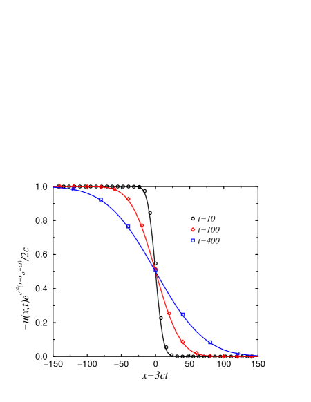
FIG. 1.: $f(y,t)=-u(x,t)\exp(c^{1/2}(x-x_{0}-ct))/2c$ vs. $y=x-3ct$ for $t=10$ (circle), 100 (diamond) and 400 (square), starting from the square-well initial condition, $u(x,0)=-V\theta(a-|x|)$, with $V=a=1$. The solid line is the analytic approximation, (5).

Separating the exponent in (16) into its real and imaginary parts, ${\cal A}(k)+i\Phi(k)$, the idea is to integrate along the contour of constant-phase $\Phi=0$ passing through the saddle point which lies on the imaginary axis. The integrand is symmetric about the imaginary axis, and is strictly decreasing as we move away from the saddle. Denoting our steepest-descent contour by $k(s)\equiv\tau(s)+i\omega(s)$, parametrized by the arclength $s$, $u$ is given by $u(x,t)=4{\cal I}(\infty)/\pi$, where

$${\cal I}(s)\equiv\int_{0}^{s}ds^{\prime}\left(\omega\frac{d\tau}{ds}+\tau\frac{d\omega}{ds}\right)\exp({\cal A}(s^{\prime}))\ .$$ (18)

We simultaneously find this steepest-descent contour and the integral $I(s)$ along the contour by solving via Runge-Kutta the following third-order system:

$$\dot{\tau} = -\Phi_{\omega}/\sqrt{\Phi_{\tau}^{2}+\Phi_{\omega}^{2}}-\lambda\Phi\Phi_{\tau}/(\Phi_{\tau}^{2}+\Phi_{\omega}^{2})$$ (19)

$$\dot{\omega} = +\Phi_{\tau}/\sqrt{\Phi_{\tau}^{2}+\Phi_{\omega}^{2}}-\lambda\Phi\Phi_{\omega}/(\Phi_{\tau}^{2}+\Phi_{\omega}^{2})$$ (20)

$$\dot{\cal I} = (-\Phi_{\omega}\omega+\Phi_{\tau}\tau)\exp({\cal A})/\sqrt{\Phi_{\tau}^{2}+\Phi_{\omega}^{2}}.$$ (21)

Here the dot denotes a derivative with respect to $s$, and $\lambda$ is an arbitrary (positive) Lagrange multiplier parameter stabilizing the $\Phi=0$ constraint. It is easy to verify that $\dot{\Phi}(k(s))=-\lambda\Phi$. In practice, $\dot{\cal I}$ decays rapidly in $s$, and the integration may be halted after sufficient accuracy is achieved. This process is easily repeated for various $x$, $t$, yielding the results in Figs. 1 and 2. In Fig. 1, we plot $f(y,t)=-u(x,t)/2c\exp(-\sqrt{c}(x-x_{0}-ct))$ for $t=10,100,400$. We also exhibit our universal approximation for $f$, (5). The argument is good for the smaller $t$, and excellent for the larger $t$’s. In Fig. 2, we again plot $f(y,t)$, this time in semi-log scale, along with our approximations (5) and (12). We see that the erfc works some way past the exponential cutoff, and that (12) works from the Gaussian regime outward, in accord with our analytical understanding.

In summary, we have found that in the KdV equation, and many other systems possessing solitons, the leading exponential edge of the soliton is only built up over time. At any given time, it is cut off at some point by a multiplicative erfc factor, which transforms the exponential decay into a Gaussian falloff. The cutoff point moves out with time, so that the length of exponential edge increases linearly with time. This cutoff phenomenon serves to give the soliton an individual identity.

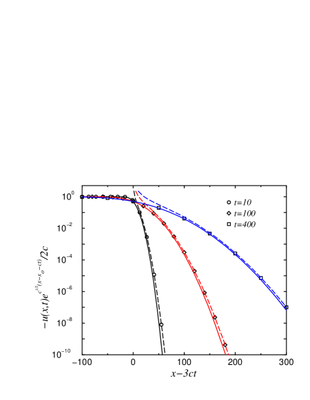
FIG. 2.: Same data as in Fig. 1, in semi-log scale, plotted together with the two overlapping approximations, (5) (solid line) and (12) (dotted line).

REFERENCES

- [1] e-mail: kessler@dave.ph.biu.ac.il
- [2] e-mail: schiff@math.biu.ac.il
- [3] D.A.Kessler, Z.Ner and L.M.Sander, preprint, archive number patt-sol/9802001.
- [4] E. Brunet and B. Derrida, Phys. Rev. E56, 2597 (1997).
- [5] U. Ebert and W. VanSaarlos, Phys. Rev. Lett. 80, 1650 (1998).
- [6] See, for example, P.G.Drazin and R.S.Johnson Solitons: an Introduction, (Cambridge University Press, Cambridge, 1989), or M.J.Ablowitz and P.A.Clarkson, Solitons, Nonlinear Evolution Equations and Inverse Scattering, London Mathematical Society Lecture Note Series volume 149, (Cambridge University Press, Cambridge, 1991).
- [7] M.J.Ablowitz and A.C.Newell, J.Math.Phys. 14 1277 (1973).
- [8] I.S.Gradshteyn and I.M.Ryzhik, Tables of Integrals, Series, and Products, Corrected and Enlarged Edition, (Academic Press, New York, 1980).