Propagation Failure in Excitable Media

Abstract

We study a mechanism of pulse propagation failure in excitable media where stable traveling pulse solutions appear via a subcritical pitchfork bifurcation. The bifurcation plays a key role in that mechanism. Small perturbations, externally applied or from internal instabilities, may cause pulse propagation failure (wave breakup) provided the system is close enough to the bifurcation point. We derive relations showing how the pitchfork bifurcation is unfolded by weak curvature or advective field perturbations and use them to demonstrate wave breakup. We suggest that the recent observations of wave breakup in the Belousov-Zhabotinsky reaction induced either by an electric field [1] or a transverse instability [2] are manifestations of this mechanism.

]

I Introduction

Failure of wave propagation in excitable media very often leads to the onset of spatio-temporal disorder. In the context of electrophysiology it may lead to ventricular fibrillation. Numerous studies have appeared in the past few years demonstrating conditions and mechanisms for failure of propagation in excitable and bistable media [3, 4, 5, 6, 7, 8, 9]. Failure may occur by external perturbations or spontaneously by intrinsic instabilities. Experimental examples include wave breakups in the excitable Belousov-Zhabotinsky (BZ) reaction induced by an electric field [1] and by a transverse instability [2].

Recently we have attributed domain breakup phenomena in bistable media to the proximity to a pitchfork front bifurcation illustrated schematically in Fig. 1a [10, 11]. As shown in Fig. 1b, near the bifurcation small perturbations, like an advective field or curvature, unfold the pitchfork bifurcation to an $S$-shaped relation. If the perturbation is large enough to drive the system past the endpoint of a given front solution branch the front reverses direction. A local reversal event along an extended front line in a two-dimensional system involves the nucleation of a pair of spiral waves and is usually followed by domain breakup. The front bifurcation illustrated in Fig. 1a has been referred to in the literature as a Nonequilibrium-Ising-Bloch (NIB) bifurcation [12, 13].

FIG. 1.: Bifurcation diagrams for fronts in the bistable FHN reaction-diffusion system. a) At the Nonequilibrium Ising-Bloch bifurcation a stationary front becomes unstable to a pair of counterpropagating fronts as a control parameter $\epsilon$ is varied. The solid lines represent a branch of front solutions with speed $c$. b) Unfolding the bifurcation near the critical point, $\epsilon_{c}$, gives an S-shaped relation in the unfolding parameter $P$.

In this paper we extend these ideas to wave breakups in excitable media. The NIB bifurcation is replaced in this case by a subcritical pitchfork pulse bifurcation as shown in Fig. 2a. The typical unfolding of that bifurcation is shown in Fig. 2b. Similar to the case of front solutions in bistable systems, perturbations that drive the system beyond the edge point of a given pulse branch may either reverse the direction of pulse propagation, or lead to pulse collapse and convergence to the stable uniform quiescent state (not shown in Fig. 2b). The convergence to a uniform attractor is more likely to occur for pulse structures than for fronts, and has always been observed in our simulations. Thus, in our study, the critical value of the bifurcation parameter, $\epsilon_{f}$, at which the upper and lower branches in Fig. 2a terminate, designates failure of propagation. Reversals in the direction of propagation (rather than collapse) have been observed in experiments on the Belousov-Zhabotinsky reaction subjected to an electric field [14].

FIG. 2.: Bifurcation diagrams for pulse solutions in the excitable FHN system. a) A typical relation for the pulse speed, $c$, vs the system parameter $\epsilon$ gives a subcritical pitchfork bifurcation. b) Unfolding the bifurcation near the critical point, $\epsilon_{c}$, gives a multiple S-shaped curve for $c$ in the unfolding parameter $P$.

In two space dimensions a local collapse of a spatially extended pulse amounts to a wave breakup. By numerically integrating a FitzHugh-Nagumo (FHN) type model, we demonstrate two scenarios of wave breakups: breakup induced by an advective field, modeling an electric field in the BZ reaction, and breakup induced by a transverse (or lateral) instability. The two scenarios, observed both in experiments [1, 2] and numerical simulations [1, 9], reflect the same mechanism: the ability of weak perturbations to drive transitions from one of the pulse branches to the uniform attractor when the system is close to failure of propagation.

In Section II we describe the derivation of a pulse bifurcation diagram for an FHN model. The derivation applies to both excitable and bistable media. The information contained in this diagram is used to draw the propagation failure line in an appropriate parameter space. In Section III we consider the unfolding of the pulse bifurcation by an advective field and demonstrate wave breakup near the propagation failure. The unfolding by curvature is studied in Section IV and wave breakup induced by a transverse instability is demonstrated. We conclude in Section V with a discussion.

II A bifurcation diagram for pulse solutions

We derive the pulse bifurcation diagram using an activator-inhibitor model of the FHN type. We assume that the activator varies on a time scale much shorter than that of the inhibitor and use singular perturbation theory [15, 16, 17]. Specifically, we study the pair of equations

$$u_{t} = \epsilon^{-1}(u-u^{3}-v)+\delta^{-1}\nabla^{2}u\,,$$ (1)

$$v_{t} = u-a_{1}v-a_{0}+\nabla^{2}v\,,$$ (2)

where $\mu=\epsilon/\delta\ll 1$ and the subscripts $t$ denote partial derivatives with respect to time. We consider a periodic wavetrain of planar (uniform along one dimension) pulses traveling at constant speed $c$ in the $x$ direction. Each of the excited (or “up state”) domains occupy a length of $\lambda_{+}$. The recovery (or “down state”) domains are of length $\lambda_{-}$. In regions where $u$ varies on a scale of order unity Eqns. (1) reduce to

$$v_{\chi\chi}+cv_{\chi}+u_{+}(v)-a_{1}v-a_{0} =0\,, \qquad-\lambda_{-}<\chi<0\,,$$ (3)

$$v_{\chi\chi}+cv_{\chi}+u_{-}(v)-a_{1}v-a_{0} =0\,, \qquad 0<\chi<\lambda_{+}\,,$$ (4)

where $\chi=x-ct$ and $u_{\pm}(v)$ are the outer solution branches of the cubic equation $u-u^{3}-v=0$. For $a_{1}$ sufficiently large we may linearize the branches $u_{\pm}(v)$ around $v=0$

$$u_{\pm}(v)\approx\pm 1-v/2\,.$$ (5)

We solve Eqns. (4) using the boundary conditions

$$v(-\lambda_{-}) = v_{b}\,,$$ (6)

$$v(0) = v_{f}\,,$$ (7)

$$v(\lambda_{+}) = v_{b}\,,$$ (8)

where $v_{f}$ and $v_{b}$ are yet undetermined, and the linear approximation (5). The solutions are

$$v = A_{+}\exp(\sigma_{1}\chi)+B_{+}\exp(\sigma_{2}\chi)+v_{+}\,,\quad-\lambda_{-}<\chi<0\,,$$

$$v = A_{-}\exp(\sigma_{1}\chi)+B_{-}\exp(\sigma_{2}\chi)+v_{-}\,,\quad 0<\chi<\lambda_{+}\,,$$

with

$$\sigma_{1,2} = -\frac{c}{2}\pm\sqrt{\frac{c^{2}}{4}+a_{1}+1/2}\,,$$ (9)

$$A_{\pm} = \frac{(v_{b}-v_{\pm})-(v_{f}-v_{\pm})\exp(\mp\sigma_{2}\lambda_{\mp})}{\exp(\mp\sigma_{1}\lambda_{\mp})-\exp(\mp\sigma_{2}\lambda_{\mp})}\,,$$ (10)

$$B_{\pm} = \frac{-(v_{b}-v_{\pm})+(v_{f}-v_{\pm})\exp(\mp\sigma_{1}\lambda_{\mp})}{\exp(\mp\sigma_{1}\lambda_{\mp})-\exp(\mp\sigma_{2}\lambda_{\mp})}\,,$$ (11)

and $v_{\pm}=(\pm 1-a_{0})/(a_{1}+1/2)$. Matching the derivatives of the solutions at $\chi=0$, $v^{\prime}(0^{-})=v^{\prime}(0^{+})$, and imposing periodicity on the derivatives, $v^{\prime}(-\lambda_{-})=v^{\prime}(\lambda_{+})$, we obtain two conditions

$$\sigma_{1}A_{+}+\sigma_{2}B_{+}=\sigma_{1}A_{-}+\sigma_{2}B_{-}\,,$$ (13)

$$\sigma_{1}A_{+}\exp(-\sigma_{1}\lambda_{-})+\sigma_{2}B_{+}\exp(-\sigma_{2}\lambda_{-}) =$$ (14)

$$\sigma_{1}A_{-}\exp(\sigma_{1}\lambda_{+})+\sigma_{2}B_{-}\exp(\sigma_{2}\lambda_{+})\,.$$ (15)

Two more conditions are obtained by studying the “front” and the “back”, that is, the leading and trailing border regions between the excited and recovery domains. Stretching the spatial coordinate according to $\zeta=\chi/\sqrt{\mu}$ gives the nonlinear eigenvalue problems

$$u_{\zeta\zeta}+c\eta u_{\zeta}+u-u^{3}-v_{f}=0\,,$$ (16)

$$u(\zeta)\to u_{-}(v_{f})\quad {\rm as} \quad\zeta\to\infty\,,$$

$$u(\zeta)\to u_{+}(v_{f})\quad {\rm as} \quad\zeta\to-\infty\,,$$

for the narrow front region, and

$$u_{\zeta\zeta}+c\eta u_{\zeta}+u-u^{3}-v_{b}=0\,,$$ (17)

$$u(\zeta)\to u_{+}(v_{b})\quad {\rm as} \quad\zeta\to\infty\,,$$

$$u(\zeta)\to u_{-}(v_{b})\quad {\rm as} \quad\zeta\to-\infty\,,$$

for the narrow back region. Here, $\eta=\sqrt{\epsilon\delta}$. Solutions of (16) and (17) yield

$$c\eta = -\frac{3}{\sqrt{2}}v_{f}\,,$$ (18)

$$c\eta = \frac{3}{\sqrt{2}}v_{b}\,,$$ (19)

respectively.

Substituting the relations (18) and (19) into Eqns. (II) leaves two equations for the three unknowns $\lambda_{+}$, $\lambda_{-}$, and $c$. The one parameter family of solutions describe periodic wavetrains of pulses traveling with speed

$$c={\cal C}(\lambda;\eta,a_{0},a_{1})\,,$$ (20)

where $\lambda=\lambda_{+}+\lambda_{-}$ is the varying wavelength of the family. The graph of $c$ versus $\lambda$ provides the dispersion relation curve obtained in earlier studies [15, 16]. Our interest here is with the behavior of a single pulse and therefore only the limit of large $\lambda$ will be considered. We remind the reader that in deriving these equations we have assumed $\mu=\epsilon/\delta\ll 1$ which excludes very small $\delta$ values.

We solved Eqns. (II) numerically for both excitable and bistable systems at large values of the period $\lambda$. The solutions were computed by numerical continuation of known solutions when $a_{0}=0$, and $\lambda_{+}=\lambda_{-}$. They yield the typical bifurcation diagram for the speed $c$ in terms of the parameter $\epsilon$ as shown in Fig. 2a. At some critical value, $\epsilon_{f}$, the branch of solutions terminates and past that point pulses fail to propagate. The value of $\epsilon_{f}$ depends on the other system parameters as well. Figure 3 shows a graph of $\epsilon=\epsilon_{f}(\delta)$ for an excitable system.

FIG. 3.: The pulse failure propagation boundary in the $\epsilon-\delta$ parameter plane for the excitable FHN model. To the right of the line pulses fail to propagate. Parameters: $a_{1}=1.25$, $a_{0}=-0.2$.

Note the inherent subcritical nature of the bifurcation [18, 19]. The bifurcation becomes supercritical only in the limit $a_{0}\to 0$ (pertaining to a bistable medium) where the pulse size tends to infinity. In that limit Eqns. (II) can easily be solved. The solutions are $c=0$ and $c=\pm\frac{2q}{\eta}\sqrt{\eta_{c}^{2}-\eta^{2}}$ for $\eta<\eta_{c}$, and coincide with the Nonequilibrium Ising-Bloch (NIB) bifurcation for front solutions [20].

III Wave breakup by an advective field

Application of an electric field to a chemical reaction involving molecular and ionic species, like the BZ reaction, results in a differential advection [21]. Differential advection in the FHN equations can be modeled (without loss of generality) by adding an advective term to the inhibitor equation

$$u_{t} = \epsilon^{-1}(u-u^{3}-v)+\delta^{-1}\nabla^{2}u\,,$$ (21)

$$v_{t} = u-a_{1}v-a_{0}+{\bf J}\cdot\nabla v+\nabla^{2}v\,,$$ (22)

where ${\bf J}$ is a constant vector. Looking for planar solutions propagating at constant speeds in the ${\bf J}$ direction, and rescaling $\epsilon$ and $\delta$ by the factor $\frac{c}{c+J}$ we find the influence on the pulse speed by the advection

$$c+J={\cal C}(\lambda;\frac{c}{c+J}\eta,a_{0},a_{1})\,,$$ (23)

where ${\cal C}$ is defined in Eqn. (20). Figures 4 show the dependence of the pulse speed $c$ on the advection constant $J$ obtained by numerically solving Eqn. (23) for large $\lambda$. Away from failure of propagation ($\epsilon$ is significantly smaller than $\epsilon_{f}$) small variations of $J$ have little effect on the pulse motion (Fig. 4a). However, close to failure, such variations can induce wave breakup by driving the system past the end point $J=J_{c}$ (Fig. 4b).

FIG. 4.: Solutions of the speed, $c$, vs advection, $J$, relation (23). (a) Away from the bifurcation point, variations in $J$ have little effect on the pulse speed ($\epsilon=0.01$). (b) Near the bifurcation point, small variations in $J$ may drive the system past the endpoint of the solution branch and cause pulse collapse ($\epsilon=0.05$). Other parameters: $a_{1}=1.25$, $a_{0}=-0.2$, $\delta=1.0$.

Figure 5 shows a numerical simulation of Eqns. (21) with ${\bf J}=J{\bf\hat{x}}$ and an initial condition of a curved pulse. Along the pulse the effective advection field is the projection of ${\bf J}$ onto the direction of propagation at that point. With $J=0$ the curved pulse propagates uniformly outward in a circular ring. Choosing $J$ slightly greater than $J_{c}$, a wave breakup results: the part of the pulse propagating in the ${\bf\hat{x}}$ direction fails to propagate. Those parts propagating in significantly different directions still propagate. These results explain earlier observations of wave breakup induced by electric fields [1].

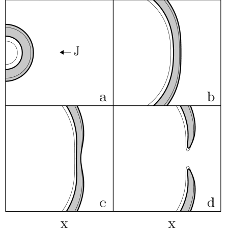
FIG. 5.: Numerical solution of Eqns. (21) with a weak advective field ${\bf J}=J{\bf\hat{x}}$. The thick and thin lines pertain to $u=0$ and $v=0$ contour lines, respectively. The initial circular pulse fails to propagate along the direction of the advective field and the pulse breaks. The pulse continues to propagate in directions different from the advective field. The equation parameters are the same as in Fig. 4.

IV Wave breakup induced by a transverse instability

Spatially extended pulses, like stripes or disks, may be unstable to transverse perturbations along the pulse line. Ohta, Mimura, and Kobayashi studied the case of deformations of planar and disk-shaped stationary patterns in a piecewise linear FitzHugh-Nagumo model [22]. Kessler and Levine derived conditions for the transverse instability of traveling stripes in a piecewise linear version of the Oregonator [23]. The curvature induced by a transverse instability can lead to the formation of labyrinthine patterns [8, 24, 25] or cause spontaneous breakup of a pulse as we will now show.

For the model of Eqns. (1), the effect of curvature $\kappa$ on pulse propagation can be obtained from Eqn. (20) by rewriting the equations in a frame moving with the pulse [26]. Assuming the radius of curvature is much larger than the pulse width, and a negligible dependence of $u$ and $v$ on arclength and time (in the moving frame) we obtain

$$\delta^{-1}u^{\prime\prime}+(c+\delta^{-1}\kappa)u^{\prime}+\epsilon^{-1}(u-u^{3}-v) = 0\,,$$ (24)

$$v^{\prime\prime}+(c+\kappa)v^{\prime}+u-a_{1}v-a_{0} = 0\,,$$ (25)

where the prime denotes differentiation with respect to a coordinate normal to the front line. Rescaling $\epsilon$ and $\delta$ by the factor $\frac{c+\delta^{-1}\kappa}{c+\kappa}$ Eqn. (20) becomes

$$c+\kappa={\cal C}(\lambda;\frac{c+\delta^{-1}\kappa}{c+\kappa}\eta,a_{0},a_{1})\,.$$ (26)

Figure 6 shows numerical solutions of Eqn. (26) for $c$ in terms of $\kappa$. Far away from failure of propagation (Fig. 6a) we find the usual approximate linear $c-\kappa$ relations for right ($c>0$) and left ($c<0$) propagating pulses [15, 17]. Close to failure (Fig. 6b), small realizable curvature variations may cause collapse.

FIG. 6.: Solutions to the speed vs curvature relation (26). (a) Away from the bifurcation point (top), the speed $c$ varies approximately linearly with the curvature $\kappa$ ($\epsilon=0.003$). (b) Near the bifurcation point, small curvature variations may drive the system past the endpoint of the solution branch and cause pulse collapse ($\epsilon=0.022$). Other parameters: $a_{1}=1.25$, $a_{0}=-0.2$, $\delta=2.5$.

Equation (26) contains information also about the transverse stability of a pulse line. A positive slope of a $c-\kappa$ relation at $\kappa=0$ indicates an instability of a planar pulse. Fig. 7 shows a simulation of Eqns. (1) at parameter values pertaining to the $c-\kappa$ relation in Fig. 6b. Starting with an near planar pulse, dents grow due to a transverse instability. The negative curvature that develops induces a wave breakup.

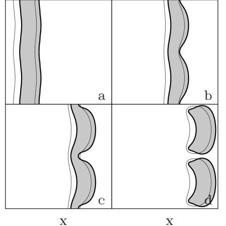
FIG. 7.: Breakup of a pulse by transverse instability. The thick and thin lines pertain to $u=0$ and $v=0$ contour lines, respectively. The initial almost planar pulse is unstable to transverse perturbations and forms a dent. The dent grows and the pulse breaks at the region of high curvature. The equation parameters are the same as in Fig. 6.

V Conclusion

We have identified a mechanism for breakup of waves in an excitable media. The key ingredient of this mechanism is the proximity to a subcritical pitchfork pulse bifurcation (as shown in Fig. 2a). Near the bifurcation small perturbations become significant and may induce failure of propagation. The nature of the perturbation is of secondary importance. As illustrated in Figs. 4b and 6b, the effects of an advective field and curvature are similar; they both induce wave breakup by driving the system past the end points of propagating pulse branches. A perturbation inducing breakup can be externally applied, like an electric field in the BZ reaction, or spontaneously formed, like curvature growth by a transverse instability. An interesting question not resolved in this study is the observed preference of propagation failure or collapse rather than reversal in the direction of propagation.

- [1] J. J. Taboada et al., Chaos 4, 519 (1994).
- [2] M. Markus, G. Kloss, and I. Kusch, Nature 371, 402 (1994).
- [3] M. Courtemanche and A. T. Winfree, Int. J. Bifurcation and Chaos 1, 431 (1991).
- [4] A. V. Holden and A. V. Panfilov, Int. J. Bifurcation and Chaos 1, 219 (1991).
- [5] A. Karma, Phys. Rev. Lett. 71, 1103 (1993).
- [6] M. Bär and M. Eiswirth, Phys Rev. E 48, R1653 (1993).
- [7] M. Bär et al., Chaos 4, 499 (1994).
- [8] A. Hagberg and E. Meron, Phys. Rev. Lett. 72, 2494 (1994).
- [9] A. F. M. Maree and A. V. Panfilov, Phys. Rev. Letters 78, 1819 (1997).
- [10] C. Elphick, A. Hagberg, and E. Meron, Phys. Rev. E 51, 3052 (1995).
- [11] A. Hagberg and E. Meron, Nonlinear Science Today (1996), (http://www.springer-ny.com/nst/).
- [12] P. Coullet, J. Lega, B. Houchmanzadeh, and J. Lajzerowicz, Phys. Rev. Lett. 65, 1352 (1990).
- [13] A. Hagberg and E. Meron, Nonlinearity 7, 805 (1994).
- [14] H. Sevcikova, M. Marek, and S. C. Muller, Science 257, 951 (1992).
- [15] J. J. Tyson and J. P. Keener, Physica D 32, 327 (1988).
- [16] J. D. Dockery and J. P. Keener, SIAM J. Appl. Math. 49, 539 (1989).
- [17] E. Meron, Physics Reports 218, 1 (1992).
- [18] P. Schütz, M. Bode, and V. V. Gafiichuk, Phys. Rev E. 52, 4465 (1995).
- [19] E. M. Kuznetsova and V. V. Osipov, Phys. Rev E. 51, 148 (1995).
- [20] A. Hagberg and E. Meron, Chaos 4, 477 (1994).
- [21] S. P. Dawson, A. Lawniczak, and R. Kapral, J. Chem Phys. 100, 5211 (1994).
- [22] T. Ohta, M. Mimura, and R. Kobayashi, Physica D 34, 115 (1989).
- [23] D. A. Kessler and H. Levine, Phys. Rev. A 41, 5418 (1990).
- [24] R. E. Goldstein, D. J. Muraki, and D. M. Petrich, Phys. Rev. E 53, 3933 (1996).
- [25] C. B. Muratov and V. V. Osipov, Phys. Rev. E 53, 3101 (1996).
- [26] A. Hagberg and E. Meron, Phys. Rev. Lett. 78, 1166 (1997).