Order Parameter Equations for Front Transitions: Nonuniformly Curved Fronts

Abstract

Kinematic equations for the motion of slowly propagating, weakly curved fronts in bistable media are derived. The equations generalize earlier derivations where algebraic relations between the normal front velocity and its curvature are assumed. Such relations do not capture the dynamics near nonequilibrium Ising-Bloch (NIB) bifurcations, where transitions between counterpropagating Bloch fronts may spontaneously occur. The kinematic equations consist of coupled integro-differential equations for the front curvature and the front velocity, the order parameter associated with the NIB bifurcation. They capture the NIB bifurcation, the instabilities of Ising and Bloch fronts to transverse perturbations, the core structure of a spiral wave, and the dynamic process of spiral wave nucleation.

1 Introduction

Interfaces separating different equilibrium or nonequilibrium states appear in a variety of contexts including crystal growth, domain walls in magnetic and hydrodynamic systems, and reaction-diffusion fronts [1]. The global patterns that appear in these systems depend to a large extent on the possible occurrence of interfacial instabilities. A transverse instability of the interface, for example, may lead to fingering and the formation of labyrinthine patterns [2, 3, 4, 5, 6, 7, 8]. Another instability with dramatic effects on pattern formation is the nonequilibrium Ising-Bloch (NIB) bifurcation [9, 10, 11, 12, 13]. The bifurcation, which takes a single stable (Ising) front to a pair of counterpropagating stable (Bloch) fronts, has been found in chemical reactions [14, 15, 16] and in liquid crystals [17, 18, 19]. Far below the NIB bifurcation stationary patterns or uniform states prevail. Far beyond it, a regime of ordered traveling patterns, including spiral waves, exists. In the vicinity of the bifurcation disordered spatio-temporal patterns, involving repeated events of spiral-wave nucleation appear. This behavior, which we call “spiral turbulence”, has been attributed to spontaneous transitions between counterpropagating Bloch fronts induced by curvature variations, front interactions, and interactions with boundaries [6, 20].

A common theoretical approach to studying pattern formation in interfacial systems is based on a geometric equation for the interface curvature (see Eqn. (2) below) [21, 22, 23, 24, 25]. Once the dependence of the normal velocity of the interface on its curvature is known the shape of the interface can be determined at any given time. For reaction-diffusion fronts this dependence may become particularly simple: Away from a NIB bifurcation, a linear relation is an excellent approximation [24, 26, 27]. The curvature equation, however, does not capture possible transitions between counterpropagating fronts near a NIB bifurcation because the front velocity becomes an independent slow degree of freedom and can no longer algebraically be related to curvature [20, 28, 29].

In this paper we consider bistable media that exhibit NIB bifurcations and derive kinematic front equations which generalize the geometric curvature equation. The new kinematic equations capture transitions between counterpropagating fronts, and spontaneous spiral-wave nucleation, a process which plays a crucial role in the onset of spiral turbulence. The equations are:

• An equation for the order parameter, $C_{0}$, associated with the NIB bifurcation:

  $${\partial C_{0}\over\partial t}=(\alpha_{c}-\alpha)C_{0}-\beta C_{0}^{3}+\gamma\kappa+\gamma_{0}+{\partial^{2}C_{0}\over\partial s^{2}}-{\partial C_{0}\over\partial s}\int_{0}^{s}\kappa C_{n}ds^{\prime}\,.$$ (1)

• A geometric equation for the front curvature, $\kappa$:

  $${\partial\kappa\over\partial t}=-(\kappa^{2}+{\partial^{2}\over\partial s^{2}})C_{n}-{\partial\kappa\over\partial s}\int_{0}^{s}\kappa C_{n}ds^{\prime}\,.$$ (2)

• An equation relating the normal front velocity $C_{n}$, the curvature $\kappa$, and the order parameter, $C_{0}$:

  $$C_{n}=C_{0}-D\kappa\,.$$ (3)

In these equations $s$ is the front arclength, and the critical parameter value, $\alpha_{c}$ designates the NIB bifurcation point. Note that Eqn. (3) cannot be regarded as a linear relation between the normal velocity of the front and its curvature since $C_{0}$ is not a constant but a dynamical variable coupled to curvature through Eqn. (1). In fact, Eqns. (1) and (3) can be recast into a single integro-differential equation for the normal velocity (using Eqn. (2))

$${\partial C_{n}\over\partial t}={\cal F}\left[C_{n},\kappa;\frac{\partial}{\partial s}\right]-{\partial C_{n}\over\partial s}\int_{0}^{s}\kappa C_{n}ds^{\prime}\,,$$ (4)

which replaces the algebraic $C_{n}-\kappa$ relation used in earlier derivations. An algebraic $C_{n}-\kappa$ relation can be recovered from Eqns. (1) and (3) assuming the order parameter $C_{0}$ follows adiabatically slow curvature variations. This issue is further discussed at the end of Section 3.

The order parameter equation (1) yields the NIB bifurcation for planar (uncurved) fronts. For a symmetric bistable system ($\gamma_{0}=0$), the Ising front, $C_{0}=0$, is stable for $\alpha>\alpha_{c}$. At $\alpha=\alpha_{c}$ the Ising front becomes unstable and a pair of Bloch fronts appears, $C_{0}=C_{0}^{\pm}\equiv\pm\sqrt{(\alpha_{c}-\alpha)/\beta}$. For a nonsymmetric system ($\gamma_{0}\neq 0$) this pitchfork bifurcation unfolds into a saddle node bifurcation in the usual way.

A brief account of the results to be reported here has appeared in Ref. [30]. We present in Section 3 a detailed derivation of the kinematic equations for a particular reaction-diffusion model introduced in Section 2. In Section 4 we study the kinematic equations. We analyze the stability of planar fronts to transverse perturbations and present numerical solutions describing steadily rotating spiral waves and spiral-wave nucleation induced by a transverse instability. We conclude in Section 5 with a discussion of our results.

2 The reaction diffusion model

We consider the FitzHugh-Nagumo model with a diffusing inhibitor,

$${\partial u\over\partial t} = \epsilon^{-1}(u-u^{3}-v)+\delta^{-1}\nabla^{2}u\,,$$

$${\partial v\over\partial t} = u-a_{1}v-a_{0}+\nabla^{2}v\,,$$ (5)

where $u$ and $v$, the activator and the inhibitor, are real scalar fields and $\nabla^{2}$ is the Laplacian operator in two dimensions. The parameter $a_{1}$ is chosen so that (5) describes a bistable medium having two stable uniform states: an up state $(u_{+},v_{+})$ and a down state $(u_{-},v_{-})$. Ising and Bloch front solutions connect the two uniform states $(u_{\pm},v_{\pm})$ as the spatial coordinate normal to the front goes from $-\infty$ to $+\infty$. The parameter space of interest is spanned by $\epsilon,\delta$ and $a_{0}$, or alternatively by $\eta=\sqrt{\epsilon\delta}$, $\mu=\epsilon/\delta$, and $a_{0}$. Note the parity symmetry $(u,v)\to(-u,-v)$ of (5) for $a_{0}=0$.

The NIB bifurcation line for $a_{0}=0$ is shown in Fig. 1. For $\mu\ll 1$ it is given by $\delta=\delta_{F}(\epsilon)=\eta_{c}^{2}/\epsilon$, or $\eta=\eta_{c}$, where $\eta_{c}=\frac{3}{2\sqrt{2}q^{3}}$ and $q^{2}=a_{1}+1/2$ [13]. The single stationary Ising front that exists for $\eta>\eta_{c}$ loses stability to a pair of counterpropagating Bloch fronts at $\eta=\eta_{c}$. Beyond the bifurcation ($\eta<\eta_{c}$) a Bloch front pertaining to an up state invading a down state coexists with another Bloch front pertaining to a down state invading an up state. Also shown in Fig. 1 are the transverse instability boundaries (for $a_{0}=0$), $\delta=\delta_{I}(\epsilon)=\epsilon/\eta_{c}^{2}$ and $\delta=\delta_{B}(\epsilon)=\eta_{c}/\sqrt{\epsilon}$, for Ising and Bloch fronts respectively. Above these lines, $\delta>\delta_{I,B}$, planar fronts are unstable to transverse perturbations [6, 31]. All three lines meet at a codimension 3 point $P3$: $\epsilon=\eta_{c}^{2}$, $\delta=1$, $a_{0}=0$.

Figure 1: The NIB front bifurcation and planar front transverse instability boundaries in the $\epsilon-\delta$ parameter plane. The thick line is the NIB bifurcation, $\delta_{F}(\epsilon)=\eta_{c}^{2}/\epsilon$. The dashed lines are the boundaries for the transverse instability of Ising, $\delta_{I}(\epsilon)$, and Bloch, $\delta_{B}(\epsilon)$, fronts. When $\delta>\delta_{I}$ ($\delta>\delta_{B}$) planar Ising (Bloch) fronts are unstable to transverse perturbations. The thin lines are approximations to the transverse instability boundaries obtained from a linear stability analysis of the kinematic equations. Parameters: $a_{1}=4.0$, $a_{0}=0$.

3 Deriving the kinematic equations

The derivation of the kinematic equations is described here in three steps: A transformation to a frame moving with the curved front (Section 3.1), derivation of the normal velocity equation (3) using a singular perturbation approach (Section 3.2), and derivation of the order parameter equation (1) (Section 3.3). In deriving the equations we assume that $\mu=\epsilon/\delta\ll 1$ and that curvature is small, $\kappa\ll 1$. Additional assumptions needed in deriving the order parameter equation are described in Section 3.3.

3.1 The moving frame

We transform to an orthogonal coordinate system $(r,s)$ that moves with the front, where $r$ is a coordinate normal to the front and $s$ is the arclength. We denote the position vector of the front by ${\bf X}(s,t)=(X,Y)$, and let it coincide with the $u=0$ contour line. The unit vectors tangent and normal to the front are given by

$${\bf\hat{s}}=\cos\theta{\bf\hat{x}}+\sin\theta{\bf\hat{y}}\,,\qquad{\bf\hat{r}}=-\sin\theta{\bf\hat{x}}+\cos\theta{\bf\hat{y}}\,,$$

where $\theta(s,t)$ is the angle that $\hat{s}$ makes with the $x$ axis. A point ${\bf x}=(x,y)$ in the laboratory frame can be expressed as

$${\bf x}={\bf X}(s,t)+r{\bf\hat{r}}\,.$$

This gives the following relation between the laboratory coordinates $(x,y)$ and the coordinates $(s,r)$ in the moving frame:

$$x=X(s,t)-r{\partial Y\over\partial s}\,,\qquad y=Y(s,t)+r{\partial X\over\partial s}\,,$$ (6)

where we used the fact that ${\bf\hat{s}}=\partial{\bf X}/\partial s$.

With this coordinate change, partial spatial derivatives transform according to

$$\frac{\partial}{\partial x}=-\frac{\partial Y}{\partial s}\frac{\partial}{\partial r}+G\frac{\partial X}{\partial s}\frac{\partial}{\partial s}\,,\qquad\frac{\partial}{\partial y}=\frac{\partial X}{\partial s}\frac{\partial}{\partial r}+G\frac{\partial Y}{\partial s}\frac{\partial}{\partial s}\,,$$ (7)

where

$$G=(1+r\kappa)^{-1}\,,$$

and $\kappa$, the front curvature, is given by

$$\kappa=-\frac{\partial\theta}{\partial s}=\frac{\partial Y}{\partial s}\frac{\partial^{2}X}{\partial s^{2}}-\frac{\partial X}{\partial s}\frac{\partial^{2}Y}{\partial s^{2}}\,.$$

The time derivative transforms according to

$${\cal D}=\frac{\partial}{\partial t}+\frac{\partial r}{\partial t}\frac{\partial}{\partial r}+\frac{\partial s}{\partial t}\frac{\partial}{\partial s}\,,$$ (8)

where  [23, 24]

$${\partial s\over\partial t} = \int_{0}^{s}\kappa C_{n}ds^{\prime}\,,$$ (9)

$${\partial r\over\partial t} = -C_{n}\,.$$ (10)

Using (7) we find for the Laplacian operator frame [32]

$$\nabla^{2}={\partial^{2}\over\partial r^{2}}+\kappa G{\partial\over\partial r}+G{\partial G\over\partial s}{\partial\over\partial s}+G^{2}{\partial^{2}\over\partial s^{2}}\,.$$ (11)

The reaction-diffusion system (5) in the moving frame is

$$\eta\sqrt{\mu}{\cal D}u = u-u^{3}-v+\mu\nabla^{2}u\,,$$

$${\cal D}v = u-a_{1}v-a_{0}+\nabla^{2}v\,,$$ (12)

where ${\cal D}$ and $\nabla^{2}$ are given by (8) and (11), respectively, and we recall that $\mu=\epsilon/\delta$ and $\eta=\sqrt{\epsilon\delta}$.

3.2 The normal velocity equation

We study Eqns. (12) assuming $\mu\ll 1$. Note that the limit $\mu\to 0$ can be taken safely without departing from the immediate neighborhood of the front bifurcation at $\eta=\eta_{c}$. We will use this fact in deriving the order parameter equation. Consider the narrow front region where $u$ changes on a spatial scale of order $\sqrt{\mu}$ while $v$ changes on a scale of order unity. Stretching the normal coordinate $r$ according to $z=r/\sqrt{\mu}$, Eqns. (12) become

$$u-u^{3}-v+\frac{\partial^{2}u}{\partial z^{2}}+\sqrt{\mu}\big{(}-\eta{\cal D}u+\kappa G\frac{\partial u}{\partial z}\bigr{)}+\mu\bigl{(}G^{2}\frac{\partial^{2}u}{\partial s^{2}}+G\frac{\partial G}{\partial s}\frac{\partial u}{\partial s}\bigr{)} = 0\,,$$

$$\frac{\partial^{2}v}{\partial z^{2}}-\mu\bigl{(}{\cal D}v+u-a_{1}v-a_{0}-G^{2}\frac{\partial^{2}v}{\partial s^{2}}-G\frac{\partial G}{\partial s}\frac{\partial v}{\partial s}\bigr{)} = 0\,.$$ (13)

Expanding $u$ and $v$ as

$$u = u_{0}+\sqrt{\mu}u_{1}+\mu u_{2}+...\,,$$

$$v = v_{0}+\sqrt{\mu}v_{1}+\mu v_{2}+...\,,$$

we find at order unity the stationary front solution

$$u_{0}=-\tanh(z/\sqrt{2}),\qquad v_{0}=0\,.$$

At order $\sqrt{\mu}$ we find the equations

$${\cal L}u_{1}=v_{1}+\eta\frac{\partial z}{\partial t}\frac{\partial u_{0}}{\partial z}-\kappa G\frac{\partial u_{0}}{\partial z}\,,\qquad\qquad\frac{\partial^{2}v_{1}}{\partial z^{2}}=0\,,$$ (14)

where

$${\cal L}=\frac{\partial^{2}}{\partial z^{2}}+1-3u_{0}^{2}\,.$$ (15)

Solvability of (14) yields

$${\partial r\over\partial t}={3\over\eta\sqrt{2}}v_{f}+\delta^{-1}\kappa\ ,$$ (16)

where $v_{f}=v(0,s,t)+{\cal O}(\epsilon^{2})$ is the approximately constant value of the inhibitor $v$ in the narrow [${\cal O}(\sqrt{\mu})$] front core region. The first term on the right-hand-side of (16) is identified with the order parameter for the NIB bifurcation: $C_{0}=-{3\over\eta\sqrt{2}}v_{f}$. Since the normal velocity is $C_{n}=-{\partial r\over\partial t}$, Eq. (16) yields the normal velocity relation (3) with $D=\delta^{-1}$.

3.3 The order parameter equation

Away from the narrow front region $u$ and $v$ change on the same spatial scales. Letting $\mu\to 0$ in Eqs. (12) we obtain $u-u^{3}-v=0$. The relevant solutions are $u=u_{+}(v)\approx 1-v/2$ for $r<0$ and $u=u_{-}(v)\approx-1-v/2$ for $r>0$ (assuming $a_{1}$ is sufficiently large) [13]. We thus obtain the following free boundary problem for $v$:

$${\cal M}v = +1-{3\over\eta\sqrt{2}}v_{f}{\partial v\over\partial r}+P_{1}+P_{2},\quad r\leq 0\,,$$

$${\cal M}v = -1-{3\over\eta\sqrt{2}}v_{f}{\partial v\over\partial r}+P_{1}+P_{2},\quad r\geq 0\,,$$ (17)

$$v(\mp\infty,s,t)=v_{\pm}={\pm 1-a_{0}\over q^{2}}\ ,$$

$$\left[v\right]_{r=0}=\left[{\partial v\over\partial r}\right]_{r=0}=0\ ,$$

where ${\cal M}={\partial\over\partial t}-{\partial^{2}\over\partial r^{2}}+q^{2},$

$$P_{1} = \left(1-\delta^{-1}\right)\kappa{\partial v\over\partial r}-a_{0}+G^{2}{\partial^{2}v\over\partial s^{2}}-{\partial s\over\partial t}{\partial v\over\partial s}\,,$$

$$P_{2} = G{\partial G\over\partial s}{\partial v\over\partial s}\,,$$

and the square brackets denote jumps of the quantities inside the brackets across the front at $r=0$.

We confine ourselves to nearly symmetric systems ($|a_{0}|\ll 1$) and to a parameter regime that includes the immediate vicinity of $P3$ and extends into the Ising regime near or below the transverse instability boundary $\delta=\delta_{I}(\epsilon)$. This allows solving the free boundary problem (17) by expanding propagating curved front solutions as power series in $c$ around the stationary planar Ising front [28, 33], where $c\ll 1$ is the speed of a planar Bloch front solution. We assume weak dependence of $\kappa$ and $v$ on $s$ and achieve this by introducing the slow length scale $S=cs$ and assuming ${\bf X}={\bf X}(S,t)$. This assumption dictates $\kappa=c^{3}\kappa_{0}$ where $\kappa_{0}\sim{\cal O}(1)$. We also introduce a slow time scale $T=c^{2}t$ to describe deviations from steady front motion. We write

$$v(r,S,t,T)=v^{(0)}(r)+\sum_{n=1}^{\infty}c^{n}v^{(n)}(r,S,t,T)\ ,$$ (18)

where

$$v^{(0)}(r) =q^{-2}(1-e^{qr})\,, \qquad r\leq 0\,,$$

$$v^{(0)}(r) =q^{-2}(e^{-qr}-1)\,, \qquad r\geq 0\,.$$

Expanding

$$\eta=\eta_{c}-c^{2}\eta_{1}+c^{4}\eta_{2}+...\,,$$

anticipating a pitchfork bifurcation, and using these expansions in (17) produces the set of equations

$$\frac{\partial v^{(n)}}{\partial t}+q^{2}v^{(n)}-\frac{\partial^{2}v^{(n)}}{\partial r^{2}}=-\rho^{(n)},~{}n=1,2,3,\ldots$$ (19)

where

$$\rho^{(1)} = {3\over\sqrt{2}\eta_{c}}v^{(1)}_{|r=0}\frac{\partial v^{(0)}}{\partial r}\,,$$ (20)

$$\rho^{(2)} = {3\over\sqrt{2}\eta_{c}}\left[v^{(1)}_{|r=0}\frac{\partial v^{(1)}}{\partial r}+v^{(2)}_{|r=0}\frac{\partial v^{(0)}}{\partial r}\right]\,,$$ (21)

$$\rho^{(3)} = +{3\eta_{1}\over\sqrt{2}\eta_{c}^{2}}v^{(1)}_{|r=0}\frac{\partial v^{(0)}}{\partial r}+{3\over\sqrt{2}\eta_{c}}\left[v^{(1)}_{|r=0}\frac{\partial v^{(2)}}{\partial r}+v^{(2)}_{|r=0}\frac{\partial v^{(1)}}{\partial r}+v^{(3)}_{|r=0}\frac{\partial v^{(0)}}{\partial r}\right]$$

$$\mbox{}+V(r,S,T)+a_{00}-(1-\delta^{-1})\kappa_{0}\frac{\partial v^{(0)}}{\partial r}\,,$$

and

$$V(r,S,T)=\frac{\partial v^{(1)}}{\partial T}-G^{2}\frac{\partial^{2}v^{(1)}}{\partial S^{2}}+\frac{\partial S}{\partial T}\frac{\partial v^{(1)}}{\partial S}\,.$$ (23)

In (3.3) we assumed $a_{0}=c^{3}a_{00}$ where $a_{00}\sim{\cal O}(1)$, and recall that $\kappa_{0}=\kappa/c^{3}$. Notice that ${\partial S\over\partial T}\sim{\cal O}(1)$, and $P_{2}$ contributes only at orders higher than $c^{3}$.

Equations (19) should be supplemented by appropriate asymptotic conditions as $r\to\pm\infty$. Since $\lim_{r\to\mp\infty}v^{(0)}(r)=\pm q^{-2}$ and $a_{0}\sim{\cal O}(c^{3})$, the asymptotic conditions in (17) are satisfied by demanding

$$\lim_{r\to\pm\infty}v^{(n)}=0\qquad n=1,2\,,$$ (24)

and

$$\lim_{r\to\pm\infty}v^{(3)}=-a_{00}/q^{2}\,.$$ (25)

We are interested in solutions of Eqns (19) at long times where they become independent of the fast time scale $t$: $\partial v^{(n)}/\partial t\to 0$ as $t\to\infty$. For $n=1$, the stationary solution of (19) with the asymptotic condition (24) is [28]

$$v^{(1)}(r,S,T)=v^{(1)}_{|r=0}F(r)\,,$$

where

$$F(r) =(1-qr)e^{qr}\,, \qquad r\leq 0\,,$$

$$F(r) =(1+qr)e^{-qr}\,, \qquad r\geq 0\,.$$

Notice that $v^{(1)}$ decays to zero as $|r|\to\infty$ on a scale of order $q^{-1}\sim{\cal O}(1)$. Since $\kappa\ll 1$ we approximated $G$ in Eqn. (23) by $G=(1+r\kappa)^{-1}\approx 1$.

For $n=2$ we obtain the stationary solution [28]

$$v^{(2)}(r,S,T)=\left[v^{(2)}_{|r=0}+{1\over 2}{v^{(1)}_{|r=0}}^{2}q^{3}r\right]F(r)\,,$$ (26)

For $n=3$, the stationary solution of (19) with (25) is

$$v^{(3)}(r,S,T)= -\frac{a_{00}}{q^{2}}+\left[v^{(3)}_{|r=0}+\frac{a_{00}}{q^{2}}+A_{+}r-B_{+}r^{2}-C_{+}r^{3}\right]e^{qr} \qquad r\leq 0\,,$$ (27)

$$v^{(3)}(r,S,T)= -\frac{a_{00}}{q^{2}}+\left[v^{(3)}_{|r=0}+\frac{a_{00}}{q^{2}}+A_{-}r-B_{-}r^{2}-C_{-}r^{3}\right]e^{-qr} \qquad r\geq 0\,,$$ (28)

where

$$A_{\pm} = q^{3}v^{(1)}_{|r=0}v^{(2)}_{|r=0}\pm\left[{3\over 4q}V(0,S,T)+{1\over 2}q^{5}{v^{(1)}_{|r=0}}^{3}\right.-\left.{q\eta_{1}\over\eta_{c}}v^{(1)}_{|r=0}-qv^{(3)}_{|r=0}+\frac{1-\delta^{-1}}{2q^{2}}\kappa_{0}\right]\,,$$

$$B_{\pm} = {1\over 4}V(0,S,T)\pm q^{4}v^{(1)}_{|r=0}v^{(2)}_{|r=0}\,,$$

$$C_{\pm} = \pm{1\over 6}q^{7}{v^{(1)}_{|r=0}}^{3}\,.$$

Application of the (no) jump condition $\bigl{[}v^{(3)}_{r}\bigr{]}_{r=0}=0$ leads to

$${\partial v^{(1)}\over\partial T}={\sqrt{2}\eta_{1}\over q\eta_{c}^{2}}v^{(1)}-{3\over 4\eta_{c}^{2}}{v^{(1)}}^{3}-{4\over 3}a_{00}-{2(1-\delta^{-1})\over 3q}\kappa_{0}+{\partial^{2}v^{(1)}\over\partial S^{2}}-{\partial S\over\partial T}{\partial v^{(1)}\over\partial S}\ ,$$ (29)

where $v^{(1)}$ is evaluated at $r=0$. Using the expansion (18), the integral (9), and transforming back to the fast variables $s,t$, Eqn. (29) becomes

$${\partial v_{f}\over\partial t}={\sqrt{2}(\eta_{c}-\eta)\over q\eta_{c}^{2}}v_{f}-{3\over 4\eta_{c}^{2}}v_{f}^{3}-{4\over 3}a_{0}\\ -{2(1-\delta^{-1})\over 3q}\kappa+{\partial^{2}v_{f}\over\partial s^{2}}-{\partial v_{f}\over\partial s}\int_{0}^{s}\kappa C_{n}ds^{\prime}\ ,$$

where $v_{f}(s,t)=v(0,s,t)$. Equation (3.3) coincides with the order parameter equation (1) once we make the following identifications: $C_{0}=-{3\over\eta\sqrt{2}}v_{f}$, $\alpha={\eta\sqrt{2}\over q\eta_{c}^{2}}$, $\alpha_{c}={\sqrt{2}\over q\eta_{c}}$, $\beta=1/6$, $\gamma=\alpha_{c}(1-\delta^{-1})$, and $\gamma_{0}=2\alpha_{c}qa_{0}$.

Algebraic $C_{n}-\kappa$ relations can be obtained from Eqns. (1) and (3) for smooth weakly curved fronts assuming $C_{0}$ follows adiabatically slow curvature variations:

$$C_{n}=C_{0}-D\kappa\,,$$ (30)

where $C_{0}$ solves

$$(\alpha_{c}-\alpha)C_{0}-\beta C_{0}^{3}+\gamma\kappa+\gamma_{0}=0\,.$$ (31)

Such an assumption is valid away from the NIB bifurcation, but the condition $C_{0}\sim c\ll 1$ used in deriving Eqn. (1) no longer holds. To test how Eqns. (30) and (31) perform away from the NIB bifurcation we compared them with $C_{n}-\kappa$ relations obtained from the implicit equation

$$C_{n}+D\kappa=\frac{3(C_{n}+\kappa)}{\sqrt{2}\eta q^{2}\sqrt{(C_{n}+\kappa)^{2}+4q^{2}}}+\frac{3a_{0}}{\sqrt{2}\eta q^{2}}\,,$$ (32)

derived in [6]. Eqn. (32) is valid at any distance from the NIB bifurcation. Figs. 2 show graphs of Eqns. (30) and (31) (solid curves) and of solutions of Eqn. (32) (dashed curves) close to and away from the NIB bifurcation. The agreement between the two approaches remains very good even where $c>1$ (Fig. 2b). Thus the adiabatic elimination of $C_{0}$ away from the bifurcation reproduces the algebraic $C_{n}-\kappa$ relations to a very good approximation.

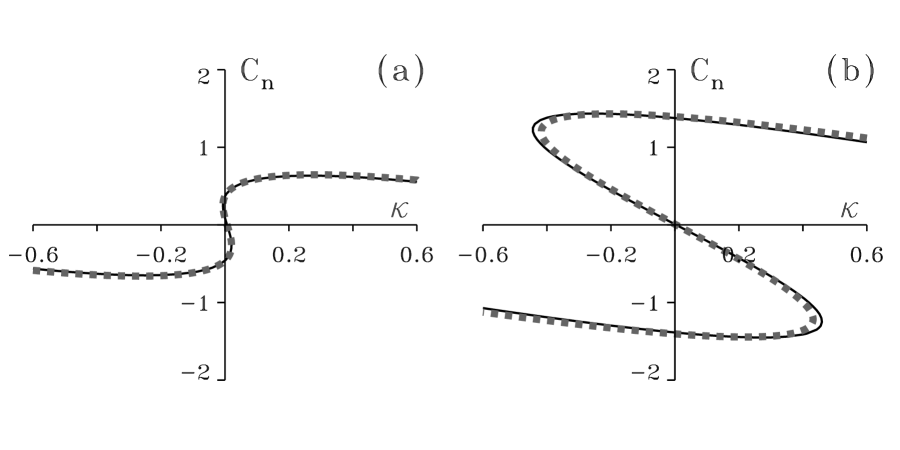
Figure 2: The $C_{n}-\kappa$ relations (30)-(31) derived from the kinematic equations (solid curve) and solutions of the implicit relation (32) (dashed line). (a) Near the NIB bifurcation, $\epsilon=0.0115$, both relations give the same result. (b) Farther from the bifurcation, $\epsilon=0.0105$, the agreement is still good even though the kinematic equations are derived for $c\ll 1$. Parameters: $a_{1}=4$, $a_{0}=-0.0001$, $\delta=1.063$.

4 Numerical solutions of the kinematic equations

We study two types of solutions to the kinematic equations: steadily rotating spiral waves (Section 4.1), and the nucleation of a spiral-wave pair by a transverse instability (Section 4.2).

4.1 Spiral waves

Consider a “front” solution connecting the planar Bloch front, $C_{0}=C_{0}^{+}$, $\kappa=0$, at $s=-\infty$ with the planar Bloch front, $C_{0}=C_{0}^{-}$, $\kappa=0$, at $s=+\infty$, where $C_{0}^{\pm}=\pm\sqrt{(\alpha_{c}-\alpha)/\beta}$, and we have assumed a symmetric model, $a_{0}=0$ or $\gamma_{0}=0$. Fig. 3a shows such a solution obtained by numerically integrating (1)-(3). As demonstrated in Fig. 3b this front solution of the kinematic equations (1)-(3) represents a spiral-wave solution of the FitzHugh-Nagumo model (5). Far away from the spiral core the leading front of the spiral approaches a planar Bloch front pertaining to an up state invading a down state ($C\to C_{0}^{+}$ as $s\to-\infty$). The trailing front approaches a planar Bloch front pertaining to a down state invading an up state ($C\to C_{0}^{-}$ as $s\to+\infty$). The spiral core is naturally captured as the interface separating these two Bloch fronts. Cores of spiral waves in bistable and excitable media have also been studied in Refs. [35, 36, 37, 38, 39, 40] using steady state free boundary formulations with linear $C_{n}-\kappa$ relations.

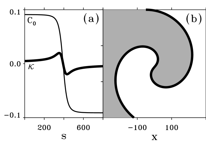
Figure 3: A front solution to the kinematic equations (1)-(3). (a) The order parameter $C_{0}$ and the curvature $\kappa$ along the arclength $s$. (b) In the $x-y$ plane the front solution corresponds to a rotating spiral wave. The shaded (light) region corresponds to an up (down) state. Parameters: $a_{1}=4.0$, $a_{0}=0$, $\epsilon=0.01234$, $\delta=1.0.$

Fig. 4a shows a similar front solution but for an asymmetric system, $a_{0}\neq 0$ or $\gamma_{0}\neq 0$. Fig. 4b shows the corresponding spiral wave. The spiral tip, defined as the point of zero curvature, is no longer stationary, but rotates along a circle. A word of caution is needed here, however. The kinematic equations do not take into account interactions between front segments. Including such interactions would require changing the asymptotic conditions, $v(\mp\infty,s,t)=v_{\pm}$ in Eqns. (17). As a result, away from the tip (outside the frame in Fig. 4b), the trailing front of the spiral meets the leading front and the up state domain disappears.

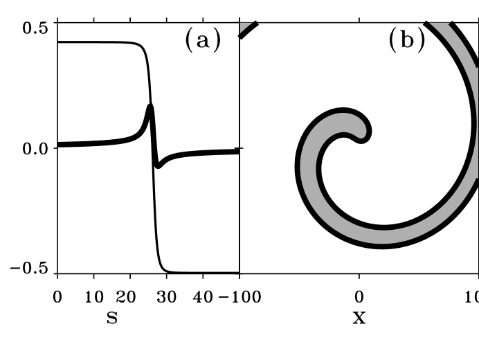
Figure 4: A front solution to the kinematic equations for a nonsymmetric system ($\gamma_{0}\neq 0$). (a) The order parameter $C_{0}$ and the curvature $\kappa$ along the arclength $s$. (b) In the $x-y$ plane the front solution corresponds to a rotating spiral wave. The shaded (light) region corresponds to an up (down) state. Parameters: $a_{1}=4.0$, $a_{0}=-0.0001$, $\epsilon=0.0115$, $\delta=1.0.$

4.2 Spiral nucleation induced by a transverse instability

Earlier numerical solutions of the FitzHugh-Nagumo model (5) revealed that an instability of a planar front solution to transverse perturbations near a NIB bifurcation can induce spontaneous nucleation of spiral waves followed by domain splitting [31]. The kinematic equations (1)-(3) capture the transverse instability of the Ising front and, to linear order around the codimension 3 point, $P3$, also the transverse instability boundary of the Bloch fronts. Explicit expressions for the transverse instability thresholds for a symmetric system ($\gamma_{0}=0$) can readily be obtained. Let

$$C_{0} = C_{0}^{0}+\bar{C}_{0}\exp(\sigma t+iQs)+c.c.$$

$$\kappa = \kappa^{0}+\bar{\kappa}\exp(\sigma t+iQs)+c.c.$$

where $(C_{0}^{0},\kappa^{0})=(0,0)$ for the Ising front and $(C_{0}^{0},\kappa^{0})=(\pm\sqrt{(\alpha_{c}-\alpha)/\beta},0)$ for the Bloch fronts. Inserting these forms in (1)-(3) gives the following transverse instability lines, linearized around $\delta=1$:

$${\rm Ising:}~{}~{}~{}\epsilon=\eta_{c}^{2}\delta\,,\qquad{\rm Bloch:}~{}~{}\epsilon=\eta_{c}^{2}(3-2\delta)\,.$$

These lines are displayed in Fig. 1 (thin lines). Fig. 5 shows typical growth rates of transverse perturbations of wavenumber $Q$ for Ising fronts (solid line) and Bloch fronts (dashed line) for the symmetric case. Note that the first wavenumber to grow as the transverse instability lines are traversed is $Q=0$, consistent with our assumption of small curvature in the vicinities of (or below) these lines.

Figure 5: Growth rates, $\sigma$, of transverse perturbations of wavenumber $Q$ to uniform solutions of the kinematic equations (1)-(3). Solid line: Bloch fronts, $\epsilon=0.011$, $\delta=1.08$. Dashed line: Ising fronts, $\epsilon=0.012$, $\delta=1.2$. In both cases $a_{1}=4.0$, $a_{0}=0$.

To test whether spiral wave nucleation induced by a transverse instability is captured by the kinematic equations, we numerically computed the time evolution of a planar front near the NIB bifurcation and beyond the transverse instability boundary. Figs. 6a-d show four snapshots of this time evolution. The initial front pertains to an up state invading a down state ($C_{0}>0$). The transverse instability causes a small dent on the front to grow (Fig. 6b). The negative curvature then triggers the nucleation of a region along the arclength where the propagation direction is reversed ($C_{0}<0$) (Fig. 6c). The pair of fronts in the kinematic equations that bound this region correspond to a pair of counter-rotating spiral waves in the FitzHugh-Nagumo equations (Fig. 6d). Fig. 6d demonstrates the equivalence of spiral pair nucleation in the bistable medium to “droplet” nucleation in the kinematic equations. The $C_{n}-\kappa$ relation for the parameter values of Figs. 6 is shown in Fig. 2a. Although the relation does not capture the nucleation dynamics it does provide a heuristic explanation of the nucleation process: the negative curvature that develops at the dent grows beyond the termination point of the upper branch in Fig. 2a and a transition to the lower branch takes place. This results in the reversal of propagation direction and the nucleation of a spiral-wave pair. The positive slopes of the upper and lower branches at $\kappa=0$ indicate transverse instabilities of the two planar Bloch front solutions.

The proximity to the front bifurcation is essential for spontaneous spiral-wave nucleation. Farther from the bifurcation initial dents may grow due to the transverse instability but not nucleate spiral waves. This is demonstrated in Figs. 7 where the same initial conditions as in Fig. 6a are chosen. The initial almost planar front develops a dent but the dent retracts rather than nucleate a spiral-wave pair.

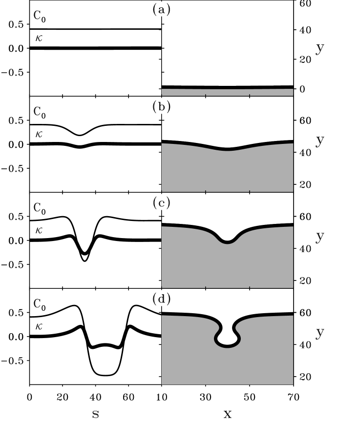
Figure 6: A numerical solution of the kinematic equations (1)-(3) demonstrating the nucleation of a spiral-wave pair from an unstable propagating front. Left column: the $C_{0}(s)$ and $\kappa(s)$ profiles. Right column: the front line shape in the $x-y$ plane. A small perturbation on the initially near planar front (a) grows (b) and nucleates a pair of spiral waves (c). The front regions in the left frame of (d) each correspond to the core of the rotating spiral in the right frame. Parameters: $a_{1}=4.0$, $a_{0}=-0.0001$, $\epsilon=0.0115$, $\delta=1.063.$ (a)-(d) are at $t=0,116,136,142$.

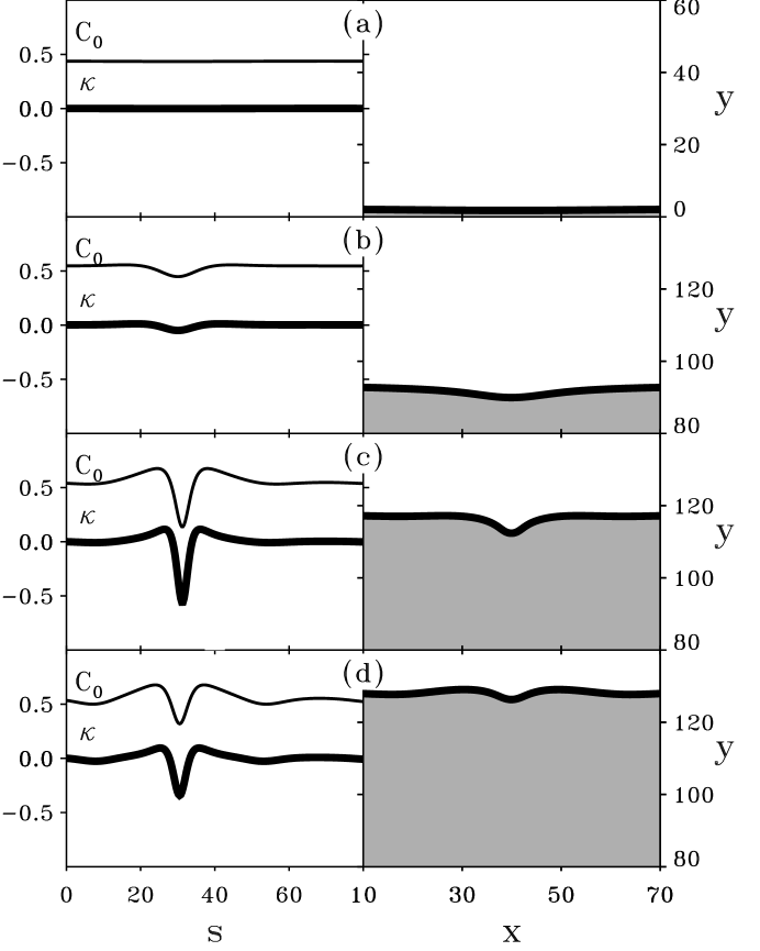
Figure 7: A numerical solution of the kinematic equations (1)-(3) with the same initial conditions as in Fig. 6 but farther away from the NIB bifurcation. Left column: the $C_{0}(s)$ and $\kappa(s)$ profiles. Right column: the front line shape in the $x-y$ plane. The transverse instability causes a small dent (a) to grow (b) but since the system is far enough from the NIB bifurcation, no spiral-wave nucleation occurs (c), and the dent contracts (d). Parameters: $a_{1}=4.0$, $a_{0}=-0.0001$, $\epsilon=0.0115$, $\delta=1.055.$ (a)-(d) are at $t=0,175,220,240$.

5 Conclusion

We have developed a new set of kinematic equations for front dynamics in nearly symmetric bistable media. The equations are quantitatively valid for slowly propagating, weakly curved fronts. They describe the growth of transverse perturbations, the core structure of spiral waves, and the dynamics of spiral-wave nucleation. Away from the NIB bifurcation, where the front velocity is no longer a slow degree of freedom, the algebraic $C_{n}$-$\kappa$ relation is recovered.

The process of spiral-wave nucleation involves local transitions between the counterpropagating Bloch fronts. In the present work these transitions were driven by curvature perturbations. Front transitions and spiral nucleation can also be driven by other intrinsic perturbations, such as nonlocal front interactions or interactions with boundaries [16]. Such interactions, however, have not been included in the present derivation. They are excluded by the choice of the boundary conditions in Eqns. (17). Front interactions are not important for the study of symmetric spirals (Figs. 3) or the initial nucleation of a spiral-wave pair from a planar front (Figs. 6). They do, however, affect nonsymmetric spiral-waves ($a_{0}\neq 0$) and might play an important role in the meander instability of a spiral tip [41, 42, 43]. Front interactions are also essential for the formation of labyrinthine patterns in the Ising regime [7].

The kinematic equations generalize an earlier approach based on a geometric equation for curvature supplemented by a linear normal velocity - curvature relation [22, 23, 24, 25]. In that case the speed of a planar front is taken to be a constant, determined by the parameters of the system, and no distinction is made between the two types of Bloch fronts. This approach has been applied to traveling waves in excitable media modeling a pulse stripe as a single curve [44, 45, 46]. It has also been applied to spiral-wave dynamics with phenomenological assumptions to describe the motion of the spiral tip, the free end of the curve [22, 23, 24, 25, 34]. No phenomenological assumptions are needed in applying the generalized kinematic equations as they naturally describe the core (or tip) structure of a spiral-wave.

Finally, we note that the two-dimensional spiral-wave nucleation problem in the original bistable medium is reduced to a one-dimensional “droplet” nucleation problem in the kinematic equations [47, 48]. This may simplify the evaluation of the critical curvature perturbation required to nucleate spiral waves.

References

- [1] M. C. Cross and P. C. Hohenberg, Rev. of Mod. Phys. 65, 2 (1993).
- [2] S. Haslam, A General History of Labyrinths (Vienna, 1888).
- [3] K. J. Lee, W. D. McCormick, Q. Ouyang, and H. L. Swinney, Science 261, 192 (1993).
- [4] J. E. Pearson, Science 261, 189 (1993).
- [5] K. J. Lee and H. L. Swinney, Phys. Rev. E 51, 1899 (1995).
- [6] A. Hagberg and E. Meron, Chaos 4, 477 (1994).
- [7] R. E. Goldstein, D. J. Muraki, and D. M. Petrich, Phys. Rev. E 53, 3933 (1996).
- [8] C. B. Muratov and V. V. Osipov, Phys. Rev. E 53, 3101 (1996).
- [9] J. Rinzel and D. Terman, SIAM J. Appl. Math 42, 1111 (1982).
- [10] H. Ikeda, M. Mimura, and Y. Nishiura, Nonl. Anal. TMA 13, 507 (1989).
- [11] P. Coullet, J. Lega, B. Houchmanzadeh, and J. Lajzerowicz, Phys. Rev. Lett. 65, 1352 (1990).
- [12] M. Bode, A. Reuter, R. Schmeling, and H.-G. Purwins, Phys Lett. A 185, 70 (1994).
- [13] A. Hagberg and E. Meron, Nonlinearity 7, 805 (1994).
- [14] G. Haas et al., Phys Rev. Lett. 75, 3560 (1995).
- [15] G. Li, Q. Ouyang, and H. L. Swinney, J. Chem. Phys 105, 10830 (1996).
- [16] D. Haim et al., Phys. Rev. Lett. 77, 190 (1996).
- [17] T. Frisch, S. Rica, P. Coullet, and J. M. Gilli, Phys. Rev. Lett. 72, 1471 (1994).
- [18] T. Frisch, Ph.D. thesis, Université de Nice Sophia-Antipolis, 1994.
- [19] S. Nasuno, N. Yoshimo, and S. Kai, Phys. Rev. E 51, 1598 (1995).
- [20] C. Elphick, A. Hagberg, and E. Meron, Phys. Rev. E 51, 3052 (1995).
- [21] R. C. Brower, D. A. Kessler, J. Koplik, and H. Levine, Phys. Rev. A 29, 1335 (1984).
- [22] V. S. Zykov, Simulation of Wave Processes in Excitable Media (Manchester University Press, Manchester, 1987).
- [23] A. S. Mikhailov, Foundation of Synergetics I: Distributed Active Systems (Springer-Verlag, Berlin, 1990).
- [24] E. Meron, Physics Reports 218, 1 (1992).
- [25] A. S. Mikhailov, V. A. Davydov, and V. S. Zykov, Physica D 70, 1 (1994).
- [26] J. J. Tyson and J. P. Keener, Physica D 32, 327 (1988).
- [27] P. Foerster, S. Müller, and B. Hess, Science 241, 685 (1988).
- [28] A. Hagberg, E. Meron, I. Rubinstein, and B. Zaltzman, Phys. Rev. E 55, 4450 (1997).
- [29] M. Bode, Physica D 106, 270 (1997).
- [30] A. Hagberg and E. Meron, Phys. Rev. Lett. 78, 1166 (1997).
- [31] A. Hagberg and E. Meron, Phys. Rev. Lett. 72, 2494 (1994).
- [32] J. P. Keener, SIAM J. Appl. Math. 39, 528 (1980).
- [33] A. Hagberg, E. Meron, I. Rubinstein, and B. Zaltzman, Phys. Rev. Lett. 76, 427 (1996).
- [34] E. Meron and P. Pelcé, Phys Rev. Lett. 60, 1880 (1988).
- [35] P. C. Fife, in Non-Equilibrium Dynamics in Chemical Systems, edited by C. Vidal and A. Pacault (Springer, Berlin, 1984), pp. 76–88.
- [36] P. Pelcé and J. Sun, Physica D 48, 353 (1991).
- [37] A. J. Bernoff, Physica D 53, 125 (1991).
- [38] A. Karma, Phys. Rev. Lett. 68, 397 (1992).
- [39] J. P. Keener, SIAM J. Appl. Math. 52, 1370 (1992).
- [40] D. A. Kessler, H. Levine, and W. N. Reynolds, Physica D 70, 115 (1994).
- [41] A. T. Winfree, Chaos 1, 303 (1991).
- [42] D. Barkley, Phys. Rev. Lett. 72, 164 (1994).
- [43] D. A. Kessler and R. Kupferman, Physica D 105, 207 (1997).
- [44] P. K. Brazhnik and J. J. Tyson, Phys. Rev. E 54, 4338 (1996).
- [45] P. K. Brazhnik, Physica D 94, 205 (1996).
- [46] V. Pérez-Muñuzuri et al., Physica D 94, 148 (1996).
- [47] P. C. Fife, Mathematical Aspects of Reacting and Diffusing Systems, Vol. 28 of Lecture Notes in Biomathematics (Springer-Verlag, New York, 1979).
- [48] J. D. Gunton and M. Droz, Introduction to the Theory of Metastable States, Vol. 183 of Lecture Notes in Physics (Springer-Verlag, Berlin, 1983).