Breaking the symmetry in bimodal frequency distributions of globally coupled oscillators

Abstract

The mean-field Kuramoto model for synchronization of phase oscillators with an asymmetric bimodal frequency distribution is analyzed. Breaking the reflection symmetry facilitates oscillator synchronization to rotating wave phases. Numerical simulations support the results based of bifurcation theory and high-frequency calculations. In the latter case, the order parameter is a linear superposition of parameters corresponding to rotating and counterrotating phases.

Collective synchronization and incoherence in large populations of nonlinearly coupled oscillators received a great attention in the recent years. Motivation for this can be found in the broad variety of phenomena which can be modeled in this framework. Indeed, synchronous flashing in swarms of fireflies [2], crickets that chirp in unison [3], epilectic seizures in the brain [4], electrical synchrony among cardiac pacemaker cells [5], arrays of Josephson junctions [6], chemical processes [7], some models of charge density waves in quasi-one-dimensional metals [8], and some neural networks used to model dynamic learning processes[9], all seem to be described in these terms.

The mathematical model conceived first as a large collection of elementary nonlinear phase oscillators, each with a globally attracting limit-cycle, goes back to Winfree [10]. It was later formulated as a system of nonlinearly coupled differential equations by Kuramoto [11], in the mean-field coupling case, and as a system of Langevin equations, (adding external white noise sources), by Sakaguchi [12],

$$\dot{\theta_{i}}=\omega_{i}+\xi_{i}(t)+\frac{K}{N}\sum_{j=1}^{N}\sin(\theta_{j}-\theta_{i}),\quad i=1,\ldots,N.$$ (1)

Here, $\theta_{i}(t)$ denotes the ith oscillator phase, $\omega_{i}$ its natural frequency (picked up from a given distribution $g(\omega)$), $K>0$ represents the coupling strength, and the $\xi_{i}$’s are independent identically distributed white noises. Consequently, the one-phase oscillator probability density, $\rho(\theta,t,\omega)$, obeys the following nonlinear Fokker-Planck equation, in the thermodynamic limit $N\to\infty$:

$$\frac{\partial\rho}{\partial t}=D\frac{\partial^{2}\rho}{\partial\theta^{2}}-\frac{\partial}{\partial\theta}(v\rho),$$ (2)

where $D>0$ comes from the noise terms in (1), and

$$v(\theta,t,\omega)=\omega+Kr\sin(\psi-\theta).$$ (3)

Here the complex-valued order parameter, $re^{i\psi}$, is defined by

$$re^{i\psi}=\int_{0}^{2\pi}\int_{-\infty}^{+\infty}e^{i\theta}\rho(\theta,t,\omega)g(\omega)d\omega d\theta.$$ (4)

It is understood that (2) must be accompanied by the prescription of the initial value $\rho(\theta,0,\omega)=\rho_{0}(\theta,\omega)$, $2\pi$-periodic boundary conditions, and normalization $\int_{0}^{2\pi}\rho(\theta,t,\omega)d\theta=1$.

The fundamental phenomenon of transition from incoherence [$\rho\equiv 1/(2\pi)$, $r\equiv 0$] to collective synchronization ($r\neq 0$) is similar to phase transitions in Statistical Physics, and it was first analyzed rigorously by Strogatz and Mirollo [13]. They studied the linear stability of incoherence of populations characterized by unimodal frequency distributions. In [14], a nonlinear stability analysis was accomplished, and bimodal frequency distributions [$g(\omega)$ with two peaks] were also considered. In the latter case, new bifurcations were discovered, showing the existence of a rich phenomenology, such as subcritical spontaneous stationary synchronization, supercritical time-periodic synchronization, bistability and hysteretic phenomena. A large amount of information was obtained in [13, 14], adopting as models of uni- and bi-modal frequency distributions, $g(\omega)=\delta(\omega)$, and $g(\omega)=\frac{1}{2}[\delta(\omega+\omega_{0})+\delta(\omega-\omega_{0})]$. It may be surprising now to realize that the asymmetric bimodal distribution,

$$g(\omega)=\alpha\delta(\omega-\omega_{0})+(1-\alpha)\delta(\omega+\omega_{0}),$$ (5)

entails essentially different features with respect to the symmetric case, $\alpha=\frac{1}{2}$, even for $\alpha$ close to $\frac{1}{2}$. Since, due to unavoidable imperfections, possibly small deviations from symmetry are most likely in Nature, the asymmetric case should be rather ubiquitous. The purpose of this paper is to illustrate the distinctive features of an asymmetric oscillator frequency distribution. The main qualitative effect of asymmetry is that no synchronized stationary phase is possible. Synchronized phases branch off from incoherence as traveling waves (TW, see below) and their structure becomes richer as the strength of the coupling increases. Asymmetry of the frequency distribution changes the stability boundaries of the incoherence (see the phase diagrams in Figs. 1 and 2), rendering it less stable, and, consequently, rendering the partially synchonized solution (whose order parameter, however, now depends always on time) more stable.

The stability boundaries for the incoherent solution, $\rho_{0}(\theta,\omega)\equiv 1/(2\pi)$ can be calculated by setting to zero the greatest of the $Re(\lambda)$’s, where $\rho=\rho_{0}+\epsilon\,e^{\lambda t}\,\eta(\theta,\omega)$ ($\epsilon\to 0$), and $\lambda$ are the eigenvalues of the linearized problem. They are given by [13]

$$\frac{x}{2}\int_{-\infty}^{+\infty}d\omega\frac{g(\omega)}{Z+i\frac{\omega}{D}}=1,$$ (6)

where we have defined $x=K/D$ and $Z=1+\lambda/D$. For the asymmetric bimodal distribution (5), we find

$$Z_{1,2}=\frac{x}{4}\pm\left[\frac{x^{2}}{16}-y^{2}+i\frac{xy}{2}(2\alpha-1)\right]^{1/2}\,,$$ (7)

where $y=\omega_{0}/D$. The stability regions in figs. 1, 2 are then determined by the condition     max $Re\ Z_{1,2}\ \leq 1$.

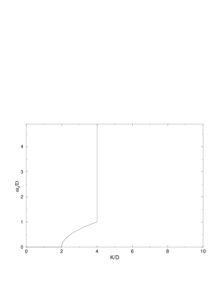
FIG. 1.: Stability boundaries for the incoherent solution for the symmetric bimodal frequency distribution. Incoherence is linearly stable in the region to the left of the solid line.

FIG. 2.: Stability boundaries for the incoherent for the asymmetric bimodal frequency distribution, $\alpha=0.49$ (solid line), $\alpha=0.3$ (dotted line).

The branch on the right of the asymptote in fig. 2 is not completely unexpected. Indeed, its counterpart in the symmetric case is a parabolic profile continuing that in fig.1 (see [14]). In the latter case, however, such a branch is not as important as in fig. 2, since it does not separate different stability regions. The behavior depicted in figs. 1 and 2 is confirmed by direct numerical simulation [17, 18] of the Kuramoto-Sakaguchi equation (2); see the evolution of the amplitude and phase of the order parameter in figs. 3, 4, and 5.

FIG. 3.: Time evolution of the amplitude $|r(t)|$ and phase $\psi(t)$ of the order parameter for $K=3,D=1,\omega_{0}=4$, with $\alpha=0.4$. Note the stability of the incoherent solution.

FIG. 4.: Time evolution of the amplitude $|r(t)|$ and phase $\psi(t)$ of the order parameter for $K=4,D=1,\omega_{0}=4$, with $\alpha=0.4$. This is the region of stability of the TW solution

FIG. 5.: Time evolution of the amplitude $|r(t)|$ and phase $\psi(t)$ of the order parameter for $K=6,D=1,\omega_{0}=4$, with $\alpha=0.4$. Another TW solution has bifurcated from incoherence resulting in a more complex behavior of the order parameter.

Observe that the phase $\psi(t)$ is always time-dependent, rather than a constant as in the case of the symmetric bimodal distribution [14, 16]. The new synchronized phases are described by a bifurcation analysis near the line in the parameter space where the incoherence loses stability:

$$\frac{\omega_{0}}{D}=\frac{2(1-\frac{K_{c}}{4D})\sqrt{\frac{K_{c}}{2D}-1}}{\sqrt{\alpha(1-\alpha)}\sqrt{(\frac{2}{\alpha}-\frac{K}{D})(\frac{2}{1-\alpha}-\frac{K}{D})}}.\,$$ (8)

This is obtained when the largest real part of the eigenvalues is set to zero, and corresponds to $K_{c}=4D$, $\omega_{0}>D$, of the symmetric case (see fig. 1). The two-time asymptotic analysis conducted in [14] may be used unchanged for bifurcations at the line (8) with the asymmetric frequency distribution, taking into account that now $\Omega^{2}=\omega^{2}+D^{2}-K_{c}D/2$, and that $g(\omega)$ is the asymmetric frequency distribution in (5). In fact, the symmetric case possesses the reflection symmetry $\omega_{0}\to-\omega_{0}$, $\theta\to-\theta$, which causes the eigenvalues to be doubly degenerated [15], whereas this is not the case for the asymmetric frequency distribution. Then, the simple analysis of Ref. [14] (which overlooked eigenvalue multiplicity, as pointed out in [15]; see also [16]) can be directly used for the asymmetric case. The result is that a branch of stable synchronized phases bifurcates from incoherence at the point given by (8). Near the bifurcation line, these solutions have the form of TWs rotating counterclockwisely [14]:

$$\rho(\theta,t,\omega)=\frac{1}{2\pi}+\frac{R\,e^{i\Psi_{0}(K-K_{c})(t-t_{0})}}{2\pi[D+i(\omega+\Omega)]}e^{i(\Omega t+\theta)}+c.c.$$ (9)

$$+O(K-K_{c}),$$ (10)

where c.c. means taking complex conjugate of the preceding term, and

$$R=\sqrt{\frac{(K-K_{c})\,\mbox{Re}\lambda_{1}}{\mbox{Re}\gamma}},\quad\Psi_{0}=\mbox{Im}\lambda_{1}-\mbox{Im}\gamma\frac{\mbox{Re}\lambda_{1}}{\mbox{Re}\gamma}\,.$$ (11)

See Ref. [14] for the explicit expressions of the parameters $\gamma$ and $\lambda_{1}=(\partial\lambda/\partial K)|_{K=K_{c}}$. In the symmetric case, another solution corresponding to waves rotating clockwisely has to be added to (9). This results in a stable standing wave solution, whose order parameter has a constant phase and an oscillatory amplitude [15, 16].

In the high-frequency limit, $\omega_{0}\rightarrow\infty$, a different perturbation analysis provides expressions for the evolution of the probability density, either near or far from bifurcation points [17]. The main result is that the frequency distribution decomposes in as many phases as peaks of the oscillator frequency distribution in such a limit. Each phase rotates with the frequency corresponding to its respective peak. Then, the order parameter may be written as a linear superposition of the order parameters of the different phases. For the asymmetric bimodal distribution, the overall order parameter evolves (except by a constant phase shift) to

$$r\,e^{i\psi}=\alpha R_{+}e^{i\omega_{0}t+\Psi_{+}}+(1-\alpha)R_{-}e^{-i\omega_{0}t+\Psi_{-}},$$ (12)

where $R_{\pm}$ and $\Psi_{\pm}$ correspond to phases rotating with angular speeds $\pm\omega_{0}$. They can be calculated with the stationary formule (2.1) and (1.7) of Ref. [14], with zero frequency [17]. Let $\alpha<1/2$ to be specific. We have the following possibilities depending on the value of the coupling constant:

1. If $0<K<2D/(1-\alpha)$, the incoherent solution $\rho_{0}\equiv 1/(2\pi)$ is stable and it is the only possible stationary solution.

2. If $2D/(1-\alpha)<K<2D/\alpha$, a globally stable partially synchronized solution branches off incoherence at $K=2D/(1-\alpha)$. It has $R_{+}=0$, $\psi=\Psi_{-}-\omega_{0}t$, and $r=(1-\alpha)\,R_{-}$. Its component $\rho_{+}\equiv 1/(2\pi)$ is incoherent, while its component $\rho_{-}$ is synchronized. The overall effect is having a TW solution (rotating clockwisely).

3. If $K>2D/\alpha$, the component $\rho_{+}$ becomes partially synchronized too. The probability density then has TW components rotating clockwisely and anticlockwisely. Their order parameters have different strengths, and $R_{-}>R_{+}$ if $\alpha<1/2$.

Let us now compare the analytical results obtained in the high-frequency limit with those obtained by means of bifurcation theory. As $\omega_{0}\to\infty$, the parameters $\lambda_{1},\gamma$, and $K_{c}$ in (11) become (cf.[14]),

$$\lambda_{1}=\frac{2D^{2}}{(1-\alpha)K_{c}^{2}}\,,\quad\gamma=\frac{1}{2D}\,,\quad K_{c}=\frac{2D}{1-\alpha}.$$ (13)

We can now calculate the order parameter in (4) by using (9), (11), and the previous expression:

$$re^{i\psi}\approx(1-\alpha)\,\left\{{K\,(1-\alpha)\over D}-2\right\}^{{1\over 2}}\,e^{-i\omega_{0}t}.$$ (14)

Eq. (14) agrees exactly with the results of the high-frequency limit (12) in [17]: The amplitude of the order parameter is constant, and its phase decreases linearly in time. Of course, for larger values of the coupling constant another branch of oscillatory solutions (TW rotating clockwisely) bifurcates from incoherence. Then, the overall probability density is richer, with an order parameter whose amplitude and phase both vary with time as in Fig. 5.

In conclusion, we have analyzed the mean-field Kuramoto-Sakaguchi model of oscillator synchronization with an asymmetric bimodal frequency distribution. In this case, reflection symmetry is broken, which results in stable synchronized phases that have the form of TWs (rotating clockwisely or anticlockwisely). These waves have order parameters with constant amplitude, and phases which depend linearly on time. As the strength of the coupling constant increases, such a synchronized phase bifurcates from incoherence. Larger values of the coupling strength result in a new bifurcation, which contributes to another TW. Then, both phase and amplitude of the order parameter become time-dependent. Numerical simulations of the model favorably agree with the results of bifurcation theory, and of high-frequency perturbation expansions. Extensions of our analyses to the case of a multimodal frequency distribution [i.e., a discrete, or a continuous $g(\omega)$ having $m$ peaks] are worth considering in future works.

This work was supported, in part by the Italian GNFM-CNR (J.A.A. and R.S.), the Fundación Carlos III de Madrid (J.A.A.), the Spanish DGES under grant PB95-0296 (L.L.B.), and the EC Human Capital and Mobility Programme under contract ERBCHRXCT930413 (S.D.L.). J.A.A. is grateful to University of “Roma Tre”, Rome, Italy, for its hospitality while Visiting Junior researcher of GNFM-CNR.

REFERENCES

- [1] E-address spigler@ulam.dmsa.unipd.it. Author to whom all correspondence should be addressed.
- [2] J.Buck, Quart. Rev. Biol. 63:265 (1988).
- [3] T.J. Walker, Science 166:891 (1969).
- [4] R.D. Traub, R. Miles, and R.K.S Wong, Science 243:1319 (1989).
- [5] D.C. Michaels, E.P. Matyas, and J.Jalife, Circulation Res. 61:704 (1987).
- [6] K. Wiesenfeld, P. Colet, and S.H. Strogatz, Phys. Rev. Lett. 76:404 (1996).
- [7] M. Scheutzow, Prob. Theory Related Fields, 72:425 (1986).
- [8] L.L. Bonilla, Phys. Rev. B 35:3637 (1987).
- [9] C.J. Pérez Vicente, A. Arenas, and L.L. Bonilla, J. Phys. A: Math. Gen. 29:L9 (1996).
- [10] A.T. Winfree, Geometry of Biological Time, Springer-Verlag, New York (1990).
- [11] Y. Kuramoto, in International Symposium of Mathematical Problems in Theoretical Physics, H. Araki ed., Lecture Notes in Physics, Vol.39 (Springer, New York), (1975).
- [12] H. Sakaguchi, Prog. Theor. Phys. 79:39 (1988).
- [13] S.H. Strogatz and R.E. Mirollo, J. Stat. Phys. 63:613 (1991).
- [14] L.L. Bonilla, J.C. Neu, and R. Spigler, J. Stat. Phys. 67:313 (1992).
- [15] J.D. Crawford, J. Stat. Phys. 74:1047 (1994).
- [16] L.L. Bonilla, C.J. Pérez Vicente, and R. Spigler, Physica D (1996) submitted.
- [17] J.A. Acebrón and L.L. Bonilla, Physica D (1997) submitted.
- [18] C.J. Pérez Vicente and F. Ritort, J. Phys. A (1996) submitted.