Phenomenological Theory for Spatiotemporal Chaos in Rayleigh-Bénard Convection

Abstract

We present a phenomenological theory for spatiotemporal chaos (STC) in Rayleigh-Bénard convection, based on the generalized Swift-Hohenberg model. We apply a random phase approximation to STC and conjecture a scaling form for the structure factor $S(k)$ with respect to the correlation length $\xi_{2}$. We hence obtain analytical results for the time-averaged convective current $J$ and the time-averaged vorticity current $\Omega$. We also define power-law behaviors such as $J\sim\epsilon^{\mu}$, $\Omega\sim\epsilon^{\lambda}$ and $\xi_{2}\sim\epsilon^{-\nu}$, where $\epsilon$ is the control parameter. We find from our theory that $\mu=1$, $\nu\geq 1/2$ and $\lambda=2\mu+\nu$ for phase turbulence and that $\mu=1$, $\nu\geq 1/2$ and $\lambda=2\mu+2\nu$ for spiral-defect chaos. These predictions, together with the scaling conjecture for $S(k)$, are confirmed by our numerical results. Finally we suggest that Porod’s law, $S(k)\sim 1/\xi_{2}k^{3}$ for large $k$, might be valid in STC.

I Introduction

Rayleigh-Bénard convection (RBC) has long been a paradigm in the study of pattern formation [2, 3]. This system consists of a thin horizontal layer of fluid heated from below. There are three dimensionless parameters to describe the system [4]. The Rayleigh number $R\equiv g\alpha d^{3}\Delta T/\kappa\nu$ is the control parameter, in which $g$ is the gravitational acceleration, $d$ the layer thickness, $\Delta T$ the temperature gradient across the layer, $\alpha$ the thermal expansion coefficient, $\kappa$ the thermal diffusivity and $\nu$ the kinematic viscosity. Under the Boussinesq approximation, only the density of the fluid is temperature dependent. Then the Prandtl number $\sigma\equiv\nu/\kappa$ is all one needs to specify the fluid properties. The third parameter is the aspect ratio $\Gamma\equiv L/d$ where $L$ is the horizontal size of the system. When the Rayleigh number $R$ surpasses a critical value $R_{c}$, the fluid bifurcates from a static conductive state to a convective state, in which the velocity profile ${\bf u}=({\bf u}_{\perp},u_{z})$ and the temperature-deviation profile $\theta$ form certain self-organized patterns. Those patterns also depend on the boundary conditions (b.c.) at the horizontal surfaces of the container. The two most studied b.c. in the literature are the rigid-rigid b.c., under which the fluid cannot slip, and the free-free b.c., under which the fluid does not experience any stress.

The patterns and the corresponding stability domain in RBC have been studied extensively in the classical work of Busse and his coauthors [5, 6] in the $(R,\sigma,k)$ space with $k$ the wavenumber. This stability domain has hence been known as the “Busse balloon” in the literature. For rigid-rigid b.c., the parallel roll state is predicted to be stable inside the Busse balloon for any given $\sigma$. Surprisingly, more recent experiments [7, 8] and numerical studies [9, 10, 11] revealed that for $\sigma\sim O(1)$ and $\Gamma\geq 50$ the parallel roll state yields to a spatiotemporally chaotic state even for states inside the Busse balloon. This spatiotemporally chaotic state, called spiral-defect-chaos (SDC), exhibits very complicated dynamics both temporally and spatially [7, 8]. Its discovery has since stimulated many experimental [7, 8, 12, 13], theoretical [14] and numerical [9, 10, 11, 15] efforts to understand it. Despite these efforts, few insights have been obtained so far.

For free-free boundaries, Zippelius and Siggia [16] and Busse and Bolton [6] found that the parallel roll state is unstable against the skewed-varicose instability immediately above onset if $\sigma<0.543$. Busse et al. [17] further investigated the dynamics involved and conjectured a direct transition from conduction to spatiotemporal chaos (STC). This spatiotemporally chaotic state is called phase turbulence (PT). Recently we reported a large scale ($\Gamma=60$) numerical simulation of the three dimensional hydrodynamical equations for $\sigma=0.5$ under the free-free b.c. [18]. From that simulation, we confirmed the direct transition to PT above onset and studied various properties of it. The patterns we found have very complicated spatial and temporal dependences.

The dynamics of the two types of STC in RBC (SDC and PT) is very complex. From the theoretical point of view, it is far from clear whether methods developed in studying ordered states, such as the Galerkin method [5, 6], the amplitude equations [19], the phase dynamics [20], etc., can be helpful at all. It seems that new concepts and new theoretical tools are needed in studying STC [21]. We know that thermodynamic systems can be characterized to a certain degree by global quantities such as temperature, pressure, density, etc.. A natural question one may ask is: Is it possible to characterize STC by some global quantities? The answer to this question is unknown at present but evidence for a positive one is very encouraging. Recently two of us found from extensive numerical studies that global quantities such as the time-averaged vorticity current and the spectrum entropy have different behaviors in the parallel roll and SDC states [15]. Furthermore, we demonstrated in our recent paper on PT [18] that both the instantaneous and the time-averaged behaviors of global quantities carry valuable information about the state. Even if global quantities may not be sufficient to describe all the dynamical details of STC, as a first step, we believe that knowledge of such quantities will broaden our understanding of STC.

The generalized Swift-Hohenberg (GSH) model of RBC [22, 23, 24] is widely accepted for theoretical study. This model is derived from the three-dimensional hydrodynamic equations, but is much simpler to study both numerically and analytically. After the corresponding $z$-dependences are separated, the vertical velocity $u_{z}({\bf r},z,t)$ and the temperature-deviation field $\theta({\bf r},z,t)$ are reduced to an order parameter $\psi({\bf r},t)$ in two-dimensional space ${\bf r}=(x,y)$, while the vertical vorticity ${\bf e}_{z}\cdot{\bf\nabla}\times{\bf u}_{\perp}({\bf r},z,t)$ is reduced to $\omega_{z}({\bf r},t)$ [22, 23, 24]. There are two coupled equations in the GSH model, one for $\psi({\bf r},t)$ and the other for $\omega_{z}({\bf r},t)$. The convective patterns in RBC are completely determined by the order parameter $\psi({\bf r},t)$. Numerical solutions of this model or its modified versions have not only reproduced most patterns observed in experiments but also resembled experimental results relatively well [2, 9, 10, 14, 15, 25]. But there are some shortcomings in the model [11, 26]: The stability boundary of the model does not coincide with that of hydrodynamics; it induces an unphysical, short-ranged cross roll instability; and both the shape and the peak position of the power spectrum for SDC are different from those in the real system. Even so, owing to its simplicity and its qualitative resemblance to real systems, this model is very valuable in studying RBC.

In this paper we present our analytical calculations, using the GSH model, of the time-averaged convective current $J=A^{-1}\int d{\bf r}\,\overline{\psi^{2}({\bf r},t)}$ and the time-averaged vorticity current $\Omega=A^{-1}\int d{\bf r}\,\overline{\omega_{z}^{2}({\bf r},t)}$ in both PT and SDC, where $\overline{F(t)}$ represents the time-average of $F(t)$ and $A$ is the area of the system. We carry out our calculations in Fourier space so the total number of modes $\hat{\psi}({\bf k},t)$ considered is infinite. By assuming the time-averaged two-point correlation function $C({\bf r}_{1},{\bf r}_{2})\equiv\overline{\psi({\bf r}_{1},t)\psi({\bf r}_{2},t)}/\overline{\psi^{2}({\bf r},t)}$ is translation invariant in STC, i.e., $C({\bf r}_{1},{\bf r}_{2})=C({\bf r}_{1}-{\bf r}_{2})$, we find that the phases of two $\hat{\psi}({\bf k},t)$ fields are uncorrelated in time unless they have the same wavenumber ${\bf k}$. Furthermore, we apply a random phase approximation (RPA) to STC in which four-point correlation functions are approximated by products of two-point correlation functions. Using this RPA, we derive $J$ and $\Omega$ in terms of the time-averaged and azimuthally averaged structure factor $S(k)\equiv\overline{\hat{\psi}^{*}({\bf k},t)\hat{\psi}({\bf k},t)}/J$. We further assume that $S(k)$ obeys a scaling form $kS(k)=\xi_{2}{\cal F}[(k-k_{max})\xi_{2}]$, in which $\xi_{2}$ is the two-point correlation length, ${\cal F}(x)$ is the scaling function and $k_{max}$ is the peak position of $kS(k)$. Applying this assumption, we obtain explicit formulas for both $J$ and $\Omega$. More precisely, we find that $J=J_{0}\epsilon-J_{\xi}\xi_{2}^{-2}$, which depends on unknown but experimentally measurable parameters, where $\epsilon=(R-R_{c})/R_{c}$ is the reduced control parameter and $J_{0}$ and $J_{\xi}$ are both known. On the other hand, we find that $\Omega=\omega_{1}J^{2}/\xi_{2}^{2}$ for rigid-rigid b.c. and $\Omega=\omega_{2}wJ^{2}/\xi_{2}$ for free-free b.c., where $w$ is related to the width of the scaling function ${\cal F}(x)$ and is experimentally measurable. The other coefficients $\omega_{1}$ and $\omega_{2}$ are known exactly. Furthermore, by assuming power law behaviors such that $J\sim\epsilon^{\mu}$, $\xi_{2}\sim\epsilon^{-\nu}$ and $\Omega\sim\epsilon^{\lambda}$, we predict from our theory that $\mu=1$, $\nu\geq 1/2$ and $\lambda=2\mu+2\nu$ for rigid-rigid b.c. and $\mu=1$, $\nu\geq 1/2$ and $\lambda=2\mu+\nu$ for free-free b.c.. This prediction and the scaling assumption for $S(k)$ have been verified by our numerical solutions for both PT and SDC.

Our paper is organized as follows. In Sec. II, we introduce the GSH model in Fourier space and derive the basic formulas governing the time-averaged convective current $J$ and the time-averaged vorticity current $\Omega$ for any pattern in RBC. We present a simple theory for PT in Sec. III. This theory is based on a conjecture of Busse et al. [17] that PT can be described by an infinite number of modes lying on a single ring in $k$-space with different orientations. Although the result for $J$ seems to agree with our numerical result extremely well, this is somewhat accidental since it predicts, incorrectly, $\Omega=0$ and also neglects the strong couplings between modes of different $k$’s. In Sec. IV we introduce the RPA of our theory and use it to calculate explicitly $J$ and $\Omega$ for both PT and SDC. The results are expressed in terms of the structure factor $S(k)$. Sec. V includes three parts. We first postulate the scaling form of the structure factor $S(k)$ and expand both $J$ and $\Omega$ in the leading order of $1/\xi_{2}$. We then define power law behaviors for $J$, $\xi_{2}$ and $\Omega$ in PT and compare the results from our theory and our numerical work [18], which agree very well for both the exponents and the amplitudes. In the last part of this section we define power law behaviors for $J$, $\xi_{2}$ and $\Omega$ in SDC and test our theoretical formulas with our numerical results [27]. The agreement between our theory and our numerical work is good in general, except for the amplitude of $\Omega$. In Sec. VI we discuss the large-$k$ behavior of the structure factor $S(k)$. We conjecture that Porod’s law [28, 29], in which $S(k)\sim 1/\xi_{S}k^{3}$ for large $k$ with $\xi_{S}$ a characteristic length, might be valid for STC. In the last section, we summarize our results and discuss some related issues.

II Basic formulas

Near the conduction to convection onset, the velocity field ${\bf u}({\bf r},z,t)=({\bf u}_{\perp},u_{z})$ and the temperature-deviation field $\theta({\bf r},z,t)$ in RBC can be approximated by [22, 23, 24]

$$\left[\begin{array}[]{c}{\bf u}_{\perp}({\bf r},z,t)\\ u_{z}({\bf r},z,t)\\ \theta({\bf r},z,t)\end{array}\right]\simeq\left[\begin{array}[]{l}u_{0}(z){\bf\nabla}\psi({\bf r},t)+\zeta_{0}(z){\bf\nabla}\zeta({\bf r},t)\times{\bf e}_{z}\\ w_{0}(z)\psi({\bf r},t)\\ \theta_{0}(z)\psi({\bf r},t)\end{array}\right],$$ (1)

where ${\bf\nabla}$ is the gradient operator in two-dimensional space ${\bf r}=(x,y)$. For both free-free boundaries at $z=0,1$ and rigid-rigid boundaries at $z=\pm\frac{1}{2}$, the explicit forms of $u_{0}(z)$, $w_{0}(z)$ and $\theta_{0}(z)$ are given in Ref. [23]; one takes $\zeta_{0}(z)=1$ for free-free boundaries and $\zeta_{0}(z)=z^{2}-\frac{1}{4}$ for rigid-rigid boundaries. Notice that the vertical vorticity ${\bf e}_{z}\cdot{\bf\nabla}\times{\bf u}_{\perp}$ is now replaced by $\zeta_{0}(z)\omega_{z}({\bf r},t)$ in which $\omega_{z}({\bf r},t)=-{{\bf\nabla}}^{2}\zeta({\bf r},t)$. Inserting Eq. (1) into the three-dimensional hydrodynamical equations in RBC and applying a few more approximations, one ends up with the two-dimensional generalized Swift-Hohenberg (GSH) model of RBC [22, 23, 24]. Although some of the approximations are not systematic, the amplitude equations for the GSH model and the hydrodynamical equations are the same in the leading order near onset. There are two coupled equations in the GSH model, one for the order parameter $\psi({\bf r},t)$ and the other for the mean-flow field $\zeta({\bf r},t)$. The convective patterns are completely determined by the order parameter $\psi({\bf r},t)$. The GSH model has been proven very successful in characterizing convective patterns under quite broad conditions [2].

In the GSH model, the order parameter $\psi({\bf r},t)$ satisfies [22, 23, 24]

$$\tau_{0}\left[\partial_{t}\psi+{\bf U}\cdot{\bf\nabla}\psi\right]=\left[\epsilon-(\xi_{0}^{2}/4k_{c}^{2})({{\bf\nabla}}^{2}+k_{c}^{2})^{2}\right]\psi-N[\psi].$$ (2)

Here $N[\psi]$ is the nonlinear term to be specified soon and ${\bf U}({\bf r})$ is the mean flow velocity given by ${\bf U}({\bf r})={\bf\nabla}\zeta({\bf r},t)\times{{\bf e}}_{z}$, in which

$$\left[\partial_{t}-\sigma({{\bf\nabla}}^{2}-c^{2})\right]{{\bf\nabla}}^{2}\zeta=g_{m}{{\bf e}}_{z}\cdot\left[{\bf\nabla}({{\bf\nabla}}^{2}\psi)\times{\bf\nabla}\psi\right].$$ (3)

In the GSH equations, the reduced Rayleigh number $\epsilon\equiv(R/R_{c})-1$ is the control parameter, in which $R$ and $R_{c}$ are the Rayleigh number and its critical value at onset. The Prandtl number $\sigma$ parameterizes the fluid. While $k_{c}$ is the critical wavenumber at onset, the other parameters model the properties of the system. The values of these parameters depend on the boundary conditions (b.c.), more precisely [23, 30],

$${\rm for\ free-free\ b.c.:\quad} R_{c}=27\pi^{4}/4,\ k_{c}=\pi/\sqrt{2},\ \tau_{0}=2(1+\sigma^{-1})/3\pi^{2},$$ (5)

$$\xi_{0}^{2}=8/3\pi^{2},\ g_{m}=6,\ c^{2}=0;$$

$${\rm for\ rigid-rigid\ b.c.:\quad} R_{c}=1707.762,\ k_{c}=3.117,\ \tau_{0}=(1+0.5117\sigma^{-1})/19.65,$$ (7)

$$\xi_{0}^{2}=0.148,\ g_{m}=24.77,\ c^{2}=10.$$

It is easier to analyze the GSH equations theoretically in Fourier space than in real space. By convention, we define the Fourier transformation and its inverse transformation of an arbitrary function $F({\bf r})$ as

$$\hat{F}({\bf k})=\frac{1}{A}\int d{\bf r}\,e^{-i{\bf k}\cdot{\bf r}}F({\bf r})\quad{\rm and}\quad F({\bf r})=\sum_{{\bf k}}\hat{F}({\bf k})e^{i{\bf k}\cdot{\bf r}},$$ (8)

where $A$ is the area of the system. Note that $\hat{F}^{*}({\bf k})=\hat{F}(-{\bf k})$ for any real function $F({\bf r})$. It is easy to check that Eq. (2) can be rewritten in Fourier space as

$$\tau_{0}\partial_{t}\hat{\psi}({\bf k})+\hat{V}({\bf k})=r(\epsilon;k)\hat{\psi}({\bf k})-\hat{N}({\bf k}),$$ (9)

where $V({\bf r})=\tau_{0}{\bf U}\cdot{\bf\nabla}\psi$ and

$$r(\epsilon;k)=\epsilon-\xi_{0}^{2}(k^{2}-k_{c}^{2})^{2}/4k^{2}_{c}.$$ (10)

Since $\psi({\bf r},t)$ is real, one has $\hat{\psi}^{*}({\bf k},t)=\hat{\psi}(-{\bf k},t)$. The nonlinear $\hat{N}({\bf k})$ term has been evaluated at onset [23],

$$\hat{N}({\bf k})=\sum_{{\bf k}_{2},{\bf k}_{3}}g(\hat{{\bf k}}\cdot\hat{{\bf k}}_{2})\hat{\psi}^{*}({\bf k}_{2})\hat{\psi}({\bf k}_{3})\hat{\psi}({\bf k}+{\bf k}_{2}-{\bf k}_{3}),$$ (11)

where the coupling constant $g(\cos\alpha)$ is given in Ref. [23] with $\alpha$ the angle between ${\bf k}$ and ${\bf k}_{2}$. Rigorously speaking, the exact forms of Eqs. (2), (3) and (11) are derived near onset and deviations from them in real physical systems are possible for large enough $\epsilon$. But we disregard such complexity and take them as our model for further study.

One may take an adiabatic approximation $(\partial_{t}=0)$ in Eq. (3) by neglecting the first term on the left-hand side. This term is small in comparison with the other terms, which can be verified by applying the same perturbation as that in phase dynamics [20]. With this approximation, it now is easy to solve Eq. (3) for $\hat{\zeta}({\bf k})$, which indicates that the mean-flow field is slaved by the $\psi({\bf r},t)$ field. We are also interested in the vertical vorticity $\omega_{z}({\bf r})=-{{\bf\nabla}}^{2}\zeta({\bf r})$. From Eq. (3), it is straightforward to get that

$$\hat{\omega}_{z}({\bf k})=k^{2}\hat{\zeta}({\bf k})=\sum_{{\bf k}_{2}}f({\bf k};{\bf k}_{2})\hat{\psi}({\bf k}_{2})\hat{\psi}({\bf k}-{\bf k}_{2}),$$ (12)

where, with an exchange of index ${\bf k}_{2}\to{\bf k}-{\bf k}_{2}$,

$$f({\bf k};{\bf k}_{2})=\frac{g_{m}}{2\sigma(k^{2}+c^{2})}(k^{2}-2{\bf k}\cdot{\bf k}_{2})({{\bf e}}_{z}\cdot{\bf k}_{2}\times{\bf k}).$$ (13)

Applying these results, one may easily evaluate the mean-flow contribution to Eq. (9), which is given by

$$\hat{V}({\bf k})=\sum_{{\bf k}_{2},{\bf k}_{3}}v({\bf k};{\bf k}_{2};{\bf k}_{3})\hat{\psi}^{*}({\bf k}_{2})\hat{\psi}({\bf k}_{3})\hat{\psi}({\bf k}+{\bf k}_{2}-{\bf k}_{3}),$$ (14)

where

$$v({\bf k};{\bf k}_{2};{\bf k}_{3})=\frac{g_{m}\tau_{0}}{2\sigma}\frac{[{{\bf e}}_{z}\cdot{\bf k}\times({\bf k}_{3}-{\bf k}_{2})][{{\bf e}}_{z}\cdot{\bf k}_{3}\times{\bf k}_{2}](k_{2}^{2}-k_{3}^{2})}{|{\bf k}_{3}-{\bf k}_{2}|^{4}+c^{2}|{\bf k}_{3}-{\bf k}_{2}|^{2}}\,.$$ (15)

Notice that the coupling constant $v({\bf k};{\bf k}_{2};{\bf k}_{3})$ is zero under two conditions: (1) If all ${\bf k}$ allowed in $\hat{\psi}({\bf k})$ point at one single direction, say $\hat{{\bf k}}$; or, (2) if all ${\bf k}$ lie on one single ring, say $|{\bf k}|=k$. For this reason, ordered states such as parallel rolls, hexagons, concentric rings, etc., do not have significant mean-flow couplings. Furthermore, the coupling constant $v({\bf k};{\bf k}_{2};{\bf k}_{3})$ seems to have a pole at ${\bf k}_{2}={\bf k}_{3}$. The real situation, however, is more subtle. Assume that ${\bf k}_{3}={\bf k}_{2}+{\bf q}$ with ${\bf q}$ very small; then $v\sim({{\bf e}}_{z}\cdot{\bf k}\times{\bf q})({{\bf e}}_{z}\cdot{\bf k}_{2}\times{\bf q})({\bf k}_{2}\cdot{\bf q})/(c^{2}q^{2}+q^{4})$. For rigid-rigid boundaries ($c^{2}=10$), there is no pole (since $v\sim q$) at $q=0$. But for free-free boundaries ($c^{2}=0$), a pole normally exists (since $v\sim 1/q$) unless ${\bf q}\|{\bf k}$, or ${\bf q}\|{\bf k}_{2}$, or ${\bf q}\perp{\bf k}_{2}$.

In this paper, we will mainly focus on two global quantities: One is the total convective current defined by

$$J(t)=\frac{1}{A}\int d{\bf r}\,\psi^{2}({\bf r},t)=\sum_{{\bf k}}\hat{J}({\bf k},t)\quad{\rm with}\quad\hat{J}({\bf k},t)=\hat{\psi}^{*}({\bf k},t)\hat{\psi}({\bf k},t);$$ (16)

the other is the total vorticity “current” defined by

$$\Omega(t) = \frac{1}{A}\int d{\bf r}\,\omega_{z}^{2}({\bf r},t)$$ (17)

$$= \sum_{{\bf k}_{1},{\bf k}_{2},{\bf k}_{3},{\bf k}_{4}}f({\bf k}_{1}+{\bf k}_{2};{\bf k}_{2})f({\bf k}_{1}+{\bf k}_{2};{\bf k}_{3})\hat{\psi}^{*}({\bf k}_{1})\hat{\psi}^{*}({\bf k}_{2})\hat{\psi}({\bf k}_{3})\hat{\psi}({\bf k}_{4})\delta_{k_{1}+{\bf k}_{2},{\bf k}_{3}+{\bf k}_{4}}.$$ (18)

Notice that $f({\bf k}_{1}+{\bf k}_{2};{\bf k}_{2})\sim(k_{1}^{2}-k_{2}^{2})({{\bf e}}_{z}\cdot{\bf k}_{2}\times{\bf k}_{1})$. So $\Omega(t)=0$ if all the wavenumbers allowed in $\hat{\psi}({\bf k})$ point at one single direction $\pm\hat{{\bf k}}$ or lie on one single ring $|{\bf k}|=k$. In other words, the vorticity current must be generated by couplings between modes of different $k$ and $\hat{{\bf k}}$. From Eq. (9), it is easy to derive that

$$\tau_{0}\partial_{t}\hat{J}({\bf k},t) = 2r(\epsilon;k)\hat{J}({\bf k},t)$$ (19)

$$- \sum_{{\bf k}_{2},{\bf k}_{3}}\left[g(\hat{{\bf k}}\cdot\hat{{\bf k}}_{2})+v({\bf k};{\bf k}_{2};{\bf k}_{3})\right]\left[\hat{\psi}^{*}({\bf k})\hat{\psi}^{*}({\bf k}_{2})\hat{\psi}({\bf k}_{3})\hat{\psi}({\bf k}+{\bf k}_{2}-{\bf k}_{3})+\mathop{\rm c.c.}\nolimits\right].$$ (20)

In principle, this is the equation determining the structure of the convective current $\hat{J}({\bf k},t)$ which, however, is beyond our present goal. Now applying the relations $\hat{\psi}^{*}({\bf k})=\hat{\psi}(-{\bf k})$ and $v({\bf k};{\bf k}_{2};{\bf k}_{3})=-v({\bf k};{\bf k}_{3};{\bf k}_{2})$, and, exchanging the summation indices ${\bf k}\to-{\bf k}$, ${\bf k}_{2,3}\to-{\bf k}_{2,3}$ for the $g$ terms and ${\bf k}\to{\bf k}+{\bf k}_{2}-{\bf k}_{3}$, ${\bf k}_{2}\leftrightarrow{\bf k}_{3}$ for the $v$ terms, one obtains from the above equation and the definition of $J(t)$ that

$$\frac{1}{2}\tau_{0}\partial_{t}J(t)=\sum_{{\bf k}}r(\epsilon;k)\hat{J}({\bf k},t)-\sum_{{\bf k}_{1},{\bf k}_{2},{\bf k}_{3}}g(\hat{{\bf k}}_{1}\cdot\hat{{\bf k}}_{2})\hat{\psi}^{*}({\bf k}_{1})\hat{\psi}^{*}({\bf k}_{2})\hat{\psi}({\bf k}_{3})\hat{\psi}({\bf k}_{1}+{\bf k}_{2}-{\bf k}_{3}).$$ (21)

This is the equation determining the total convective current $J(t)$. Notice that the $v$ terms vanish from this equation, which can also be derived directly from Eq. (2) by converting the corresponding integral in Eq. (16) into a surface term. In general, the $v$ couplings affect $J(t)$ implicitly by modifying its structure $\hat{J}({\bf k},t)$ unless, of course, $v\equiv 0$.

For stationary states, the convective current and the vorticity current are time-independent. This, however, is no long true if the state is spatiotemporal chaotic. For a spatiotemporal chaotic state, these two currents normally fluctuate in time around some well-defined averaged values: see Refs. [15, 18]. While the fluctuations appear chaotic in time, they are relatively small in comparison with their averaged values. For simplicity, we only consider the two corresponding time-averaged currents in our theory. We now introduce the time-average operator $\cal T$ defined by

$${\cal T}F(t)\equiv\overline{F(t)}=\lim_{T\to+\infty}\frac{1}{T}\int^{T}_{0}dtF(t).$$ (22)

Applying $\cal T$ to Eq. (21) yields

$$\sum_{{\bf k}}r(\epsilon;k)\overline{\hat{J}({\bf k},t)}-\sum_{{\bf k}_{1},{\bf k}_{2},{\bf k}_{3},{\bf k}_{4}}g(\hat{{\bf k}}_{1}\cdot\hat{{\bf k}}_{2})\overline{\hat{\psi}^{*}({\bf k}_{1})\hat{\psi}^{*}({\bf k}_{2})\hat{\psi}({\bf k}_{3})\hat{\psi}({\bf k}_{4})}\,\delta_{{\bf k}_{1}+{\bf k}_{2},{\bf k}_{3}+{\bf k}_{4}}=0.$$ (23)

In the next several sections, we show how, under various assumptions, to calculate the time-averaged convective current of STC from this equation. The time-averaged vorticity current can be obtained with $\cal T$ acting on Eq. (18). For simplicity, we denote from now on $\hat{J}({\bf k})=\overline{\hat{J}({\bf k},t)}$, $J=\overline{J(t)}$ and $\Omega=\overline{\Omega(t)}$.

Finally we introduce the time-averaged structure factor defined by

$$\hat{S}({\bf k})=\hat{J}({\bf k})/J\quad{\rm with}\quad\sum_{{\bf k}}\hat{S}({\bf k})=1,$$ (24)

and the corresponding averages

$$\langle\hat{F}\rangle_{\bf k}=\sum_{{\bf k}}\hat{S}({\bf k})\hat{F}({\bf k}).$$ (25)

With this notation, the first term in Eq. (23) can be rewritten as $\langle r(\epsilon)\rangle_{\bf k}J$. If the $k$-dependence and the angular dependence in $\hat{S}({\bf k})$ can be separated, then it is more convenient to define

$$\hat{S}({\bf k})=(2\pi)^{2}A^{-1}S(k)\Phi(\alpha)\quad{\rm with}\quad\int^{\infty}_{0}dk\,kS(k)=1\quad{\rm and}\quad\int^{2\pi}_{0}d\alpha\,\Phi(\alpha)=1,$$ (26)

where $\alpha$ is the angle between ${\bf k}$ and some reference direction. Here the discrete ${\bf k}$ lattice has been converted into a continuous one. So a proper phase factor has been taken into account. Notice also that $\Phi(\pi+\alpha)=\Phi(\alpha)$ since $\hat{S}(-{\bf k})=\hat{S}({\bf k})$. Now the corresponding averages with respect to $S(k)$ and $\Phi(\alpha)$ are defined as

$$\langle F\rangle_{k}=\int^{\infty}_{0}dk\,kS(k)F(k)\quad{\rm and}\quad\langle F\rangle_{\alpha}=\int^{2\pi}_{0}d\alpha\,\Phi(\alpha)F(\alpha).$$ (27)

For $\hat{F}({\bf k})=F(k,\alpha)$, it is easy to see that $\langle\hat{F}\rangle_{\bf k}=\langle F\rangle_{k,\alpha}$ if a separation like Eq. (26) holds.

III A Simple Theory for PT

In order to calculate the time-averaged convective current and the time-averaged vorticity current from Eqs. (23) and (18), it is obvious that more information about the corresponding state is needed. We now present a simple model for PT, following a conjecture by Busse and his coauthors [17], and calculate the corresponding convective current. For this task, we notice first that a PT state consists of many superimposed rolls with different orientations [17, 18], among which no particular direction is preferred. On the other hand, since this PT occurs immediately above the onset [6, 16, 17, 18], the amplitude of the wave number $k$ lies in the vicinity of $k_{c}$. Our numerical simulations [18] also revealed that the time-averaged structure factor is isotropic azimuthally.

As a first attempt, we assume that a PT state is composed of many parallel rolls, whose wave numbers lie on a ring and whose amplitudes are equal. More precisely, we assume that

$$\hat{\psi}({\bf k},t)=\psi_{0}(t)\,\delta_{k,q}\sum^{M}_{i=1}e^{i\phi(\beta_{i},t)}\delta_{\alpha,\beta_{i}(t)}\,,$$ (28)

where $\psi_{0}(t)$ and $\phi(\beta_{i},t)$ are the amplitude and the phases of those selected modes, $q(\simeq k_{c})$ and $\beta_{i}(t)$ are the amplitude and the angles of their corresponding wave numbers, while $M$ is the total number of those modes, and $\alpha$ is the angle between ${\bf k}$ and some reference direction. From Eq. (16), one finds that $J(t)=\sum_{{\bf k}}|\hat{\psi}({\bf k},t)|^{2}=M\psi^{2}_{0}(t)$. One has $M=2$, $\psi_{0}=\sqrt{J/2}$, $\phi(\beta_{i},t)={\rm const.}$, and $\beta_{i}=i\pi$ with $i=0,1$ for parallel rolls, and $M=6$, $\psi_{0}=\sqrt{J/6}$, $\phi(\beta_{i},t)={\rm const.}$, and $\beta_{i}=i\pi/3$ with $i=0,1,\cdots,5$ for hexagons [23]. For PT, we take $M\to+\infty$. Since $J(t)$ in PT has a well-defined time-averaged value with small fluctuations [18], we expect the same behavior for $\psi_{0}(t)$. But we speculate that both the phases $\phi(\beta_{i},t)$ and the angular distribution $\{\beta_{i}(t)\}$ are irregular in time, which leads to the spatiotemporal chaotic behavior in PT. From $\hat{\psi}^{*}({\bf k},t)=\hat{\psi}(-{\bf k},t)$, one finds that if $\beta_{i}(t)$ is selected, so must be $\pi+\beta_{i}(t)$ with $\phi(\pi+\beta_{i},t)=-\phi(\beta_{i},t)$.

We now use this model to calculate the time-averaged convective current from Eq. (23). While the first term can be easily evaluated as $r(\epsilon,q)J$, the second term is much more complicated. Notice that the condition ${\bf k}_{1}+{\bf k}_{2}={\bf k}_{3}+{\bf k}_{4}$ imposes a very strong constraint on the available wave numbers on a ring. There are only three possibilities for the condition to be satisfied, see Fig. 1: (a) If ${\bf k}_{1}+{\bf k}_{2}=0$, then ${\bf k}_{3}+{\bf k}_{4}=0$; (b) if ${\bf k}_{1}\neq{\bf k}_{2}$ and ${\bf k}_{1}+{\bf k}_{2}\neq 0$, then either ${\bf k}_{3}={\bf k}_{1}$ and ${\bf k}_{4}={\bf k}_{2}$ or ${\bf k}_{3}={\bf k}_{2}$ and ${\bf k}_{4}={\bf k}_{1}$; or, (c) if ${\bf k}_{1}={\bf k}_{2}$, then ${\bf k}_{3}={\bf k}_{4}={\bf k}_{1}$. It is more convenient to express these constraints in terms of their angles, which can be summarized, correspondingly, as: (a) $\delta_{\alpha_{2},\alpha_{1}+\pi}\delta_{\alpha_{4},\alpha_{3}+\pi}$, (b) $(1-\delta_{\alpha_{2},\alpha_{1}+\pi}-\delta_{\alpha_{2},\alpha_{1}})(\delta_{\alpha_{3},\alpha_{1}}\delta_{\alpha_{4},\alpha_{2}}+\delta_{\alpha_{3},\alpha_{2}}\delta_{\alpha_{4},\alpha_{1}})$, and (c) $\delta_{\alpha_{2},\alpha_{1}}\delta_{\alpha_{3},\alpha_{1}}\delta_{\alpha_{4},\alpha_{1}}$. Now inserting Eq. (28) into the second term of Eq. (23) and applying $\phi(\beta_{i}+\pi)=-\phi(\beta_{i},t)$ and these constraints, after some algebra, one finds that the second term is simply $-M^{2}g_{M}\overline{\psi^{4}_{0}(t)}$ with

$$g_{M}=g(-1)(1-\frac{2}{M})-\frac{1}{M}g(1)+\frac{2}{M^{2}}\sum^{M}_{i,j=1}\overline{g[\cos(\beta_{i}(t)-\beta_{j}(t))]}.$$ (29)

Here $\overline{\psi_{0}^{4}(t)}$ and $\overline{g[\cos(\beta_{i}(t)-\beta_{j}(t))]}$ have been decoupled, which seems reasonable. Since $J=M\overline{\psi^{2}_{0}(t)}$, if one neglects the fluctuations of $\psi_{0}(t)$, one has then $M^{2}\overline{\psi^{4}(t)}\simeq J^{2}$. From Eq. (23), this leads to the solution for the total time-averaged convective current

$$J\simeq r(\epsilon,q)/g_{M},$$ (30)

in addition to the conduction solution $J=0$. This solution reproduces the known results [23] for both parallel rolls with $g_{2}=g(-1)+\frac{1}{2}g(1)$ and hexagons with $g_{6}=\frac{1}{6}[6g(-1)+4g(-\frac{1}{2})+4g(\frac{1}{2})+g(1)]$.

For PT, we expect that $\beta_{i}(t)$ and $\beta_{j}(t)$ are uncorrelated in time and that fluctuations of $\beta_{i}(t)$ can be neglected such that $\overline{\beta_{i}^{n}(t)}\simeq\overline{\beta_{i}(t)}^{n}$ for any positive integer $n$. So we may make another approximation such that $\overline{g[\cos(\beta_{i}(t)-\beta_{j}(t))]}\simeq g[\cos(\overline{\beta_{i}(t)}-\overline{\beta_{j}(t)})]$, where $\{\overline{\beta_{i}(t)}\}$ should be uniformly distributed between $[0,2\pi]$. From this approximation and $\sum_{i=1}^{M}\to(M/2\pi)\int^{2\pi}_{0}d\alpha$ as $M\to+\infty$, one finds that

$$g_{\infty}=g(-1)+\frac{2}{\pi}\int^{\pi}_{0}d\alpha\,g(\cos\alpha).$$ (31)

Using the explicit formula given in Ref. [23] for free-free boundaries, one has finally that

$$g_{PT}=0.855922+0.0458144\sigma^{-1}+0.0709326\sigma^{-2},$$ (32)

where $\sigma$ is the Prandtl number. Since typically $q\simeq k_{c}(1+q_{0}\epsilon)$, one finds that the time-averaged convective current $J\simeq r(\epsilon,q)/g_{\rm PT}\simeq\epsilon/g_{PT}$ in PT, recalling Eq. (10). For $\sigma=0.5$, this simple theory gives $g_{PT}\simeq 1.2313$. In comparison, we found $g_{PT}\simeq 1.27\pm 0.03$ from our three-dimensional numerical calculations [18]. Considering all the approximations we have made, such a good agreement is very encouraging.

However, this simple model apparently misses two important features of PT. The first is the lack of the vorticity current. Since all ${\bf k}$ lie on a single ring in our model, the vorticity current is identically zero from our discussions in the previous section. This, however, is not born out by our numerical calculations. Secondly, the structure factor from our numerical calculations has a finite width near its peak position, which leads to a significant reduction on the value of $J$ as shown in Sec. V. So it is inaccurate to assume $|{\bf k}|=q$ for all ${\bf k}$. To improve it, we now discuss a more physically sound theory.

IV Random Phase Approximation for STC

A Convective Current

We now consider a different approach to STC (both PT and SDC) in RBC. For this purpose, we notice that although the instantaneous patterns in STC are irregular and random in space [7, 8, 9, 10, 11, 18], some spatial symmetries can be restored if the system is averaged over a very long time. For example, for a laterally infinite system, it seems natural to assume that the time-averaged quantity $\overline{\psi^{2}({\bf r},t)}$ is uniform in space and that the two-point correlation function, defined as $C({\bf r}_{1},{\bf r}_{2})\equiv\overline{\psi({\bf r}_{1},t)\psi({\bf r}_{2},t)}/\overline{\psi^{2}({\bf r}_{1},t)}$, is translation invariant, i.e., $C({\bf r}_{1},{\bf r}_{2})=C({\bf r}_{1}-{\bf r}_{2})$. Then, one finds from Eq. (16) that $\overline{\psi^{2}({\bf r},t)}=J$, and, from Eqs. (8) and (24) that

$$\overline{\hat{\psi}^{*}({\bf k}_{1},t)\hat{\psi}({\bf k}_{2},t)}=J\delta_{{\bf k}_{1},{\bf k}_{2}}\hat{S}({\bf k}_{1}).$$ (33)

It is also easy to check that $\hat{S}({\bf k})$ is just the Fourier component of $C({\bf r})$.

To understand the physical implications of the above result, we assume that

$$\hat{\psi}({\bf k},t)=\hat{\rho}({\bf k},t)e^{i\hat{\phi}({\bf k},t)},$$ (34)

with both $\hat{\rho}({\bf k},t)$ and $\hat{\phi}({\bf k},t)$ real. Since $\hat{\psi}^{*}({\bf k},t)=\hat{\psi}(-{\bf k},t)$, one has $\hat{\rho}(-{\bf k},t)=\hat{\rho}({\bf k},t)$, $\hat{\phi}(-{\bf k},t)=-\hat{\phi}({\bf k},t)$ and $\hat{J}({\bf k})=\overline{\hat{\rho}^{2}({\bf k},t)}$. While both experimental measurements and numerical calculations suggest that the amplitude has a well-defined time-averaged value with small fluctuations, the phase seems to have a rather complicated, irregular time-dependence. If the amplitude and the phase can be assumed to be uncorrelated in time, the above result indicates that phases of different modes are totally uncorrelated in time. Since the $\delta_{{\bf k}_{1},{\bf k}_{2}}$ factor in Eq. (33) can be represented by

$$\delta_{{\bf k}_{1},{\bf k}_{2}}=(2\pi)^{2}A^{-1}\delta({\bf k}_{1}-{\bf k}_{2})=\lim_{\xi_{\phi}\to+\infty}(2\pi\xi^{2}_{\phi}/A)\exp[-\frac{1}{2}({\bf k}_{1}-{\bf k}_{2})^{2}\xi^{2}_{\phi}],$$ (35)

we hence adapt a random phase approximation (RPA) to STC in which

$$\overline{\exp[-i\hat{\phi}({\bf k}_{1},t)+i\hat{\phi}({\bf k}_{2},t)]}=\exp[-\frac{1}{2}({\bf k}_{1}-{\bf k}_{2})^{2}\xi^{2}_{\phi}].$$ (36)

Here $\xi_{\phi}$ is a length determining the correlation between phases of different modes. We expect that $\xi_{\phi}=[A/2\pi]^{1/2}\to+\infty$ for a laterally infinite system but, as we will show, this limit should be taken only later on.

Now, since the phases are random in time, one may further approximate a four-phase correlation by products of two-phase correlations, i.e.,

$$\overline{\exp[-i\hat{\phi}({\bf k}_{1},t)-i\hat{\phi}({\bf k}_{2},t)+i\hat{\phi}({\bf k}_{3},t)+i\hat{\phi}({\bf k}_{4},t)]}$$ (37)

$$\simeq\overline{\exp[-i\hat{\phi}({\bf k}_{1},t)-i\hat{\phi}({\bf k}_{2},t)]}\ \overline{\exp[i\hat{\phi}({\bf k}_{3},t)+i\hat{\phi}({\bf k}_{4},t)]}$$ (38)

$$\quad+\overline{\exp[-i\hat{\phi}({\bf k}_{1},t)+i\hat{\phi}({\bf k}_{3},t)]}\ \overline{\exp[-i\hat{\phi}({\bf k}_{2},t)+i\hat{\phi}({\bf k}_{4},t)]}$$ (39)

$$\quad+\overline{\exp[-i\hat{\phi}({\bf k}_{1},t)+i\hat{\phi}({\bf k}_{4},t)]}\ \overline{\exp[-i\hat{\phi}({\bf k}_{2},t)+i\hat{\phi}({\bf k}_{3},t)]}$$ (40)

$$=\exp\left[-\frac{1}{2}({\bf k}_{1}+{\bf k}_{2})^{2}\xi^{2}_{\phi}-\frac{1}{2}({\bf k}_{3}+{\bf k}_{4})^{2}\xi^{2}_{\phi}\right]+\exp\left[-\frac{1}{2}({\bf k}_{1}-{\bf k}_{3})^{2}\xi^{2}_{\phi}-\frac{1}{2}({\bf k}_{2}-{\bf k}_{4})^{2}\xi^{2}_{\phi}\right]$$ (41)

$$\quad+\exp\left[-\frac{1}{2}({\bf k}_{1}-{\bf k}_{4})^{2}\xi^{2}_{\phi}-\frac{1}{2}({\bf k}_{2}-{\bf k}_{3})^{2}\xi^{2}_{\phi}\right].$$ (42)

Applying this and neglecting the correlations of $\hat{J}({\bf k},t)$ such that $\overline{\hat{J}({\bf k}_{1},t)\hat{J}({\bf k}_{2},t)}\simeq\hat{J}({\bf k}_{1})\hat{J}({\bf k}_{2})$, one may rewrite Eq. (23) in a continuous Fourier space as

$$\langle r(\epsilon,k)\rangle_{\bf k}J=\frac{A^{4}}{(2\pi)^{8}}\int d{\bf k}_{1}d{\bf k}_{2}d{\bf k}_{3}d{\bf k}_{4}\,\frac{(2\pi)^{2}}{A}\delta({\bf k}_{1}+{\bf k}_{2}-{\bf k}_{3}-{\bf k}_{4})\,g(\hat{{\bf k}}_{1}\cdot\hat{{\bf k}}_{2})$$ (43)

$$\hskip 60.00009pt\times\left[\hat{J}({\bf k}_{1})\hat{J}({\bf k}_{3})e^{-\frac{1}{2}({\bf k}_{1}+{\bf k}_{2})^{2}\xi^{2}_{\phi}-\frac{1}{2}({\bf k}_{3}+{\bf k}_{4})^{2}\xi^{2}_{\phi}}+\hat{J}({\bf k}_{1})\hat{J}({\bf k}_{2})e^{-\frac{1}{2}({\bf k}_{1}-{\bf k}_{3})^{2}\xi^{2}_{\phi}-\frac{1}{2}({\bf k}_{2}-{\bf k}_{4})^{2}\xi^{2}_{\phi}}\right.$$ (44)

$$\hskip 72.00008pt\left.+\hat{J}({\bf k}_{1})\hat{J}({\bf k}_{2})e^{-\frac{1}{2}({\bf k}_{1}-{\bf k}_{4})^{2}\xi^{2}_{\phi}-\frac{1}{2}({\bf k}_{2}-{\bf k}_{3})^{2}\xi^{2}_{\phi}}\right].$$ (45)

Since $\xi_{\phi}\to+\infty$, we may take $g(\hat{{\bf k}}_{1}\cdot\hat{{\bf k}}_{2})=g(-1)$ for the first term on the right hand side. Then, after some algebra, one finds that

$$J=\frac{4\pi\xi_{\phi}^{2}}{A}\frac{\langle r(\epsilon,k)\rangle_{k}}{g_{\infty}}=\frac{2\langle r(\epsilon,k)\rangle_{k}}{g_{\infty}},$$ (46)

in addition to the conduction solution $J=0$. Here $A=2\pi\xi_{\phi}^{2}$ has been used, $\hat{S}({\bf k})$ is assumed to be azimuthally uniform, and $g_{\infty}$ is defined in Eq. (31). Notice that this result is valid for both PT and SDC, but the exact values of $g_{\infty}$ and $\langle r(\epsilon,k)\rangle_{k}$ depends on the boundary conditions. While the value of $g_{\infty}$ for PT has been given in Eq. (32), the corresponding value for SDC is

$$g_{SDC}=1.1319+0.0483\sigma^{-1}+0.0710\sigma^{-2},$$ (47)

which is obtained by interpolating the data for $g(\cos\alpha)$ given in Ref. [23] for rigid-rigid boundaries and by integrating the consequent fitting function.

It is worthwhile to point out that if one takes the limit $\xi_{\phi}\to+\infty$ as early as in Eq. (42), one misses the factor $2$ in Eq. (46). To understand this, one should notice that Eq. (42) reduces to $\delta_{{\bf k}_{1},-{\bf k}_{2}}\delta_{{\bf k}_{3},-{\bf k}_{4}}+\delta_{{\bf k}_{1},{\bf k}_{3}}\delta_{{\bf k}_{2},{\bf k}_{4}}+\delta_{{\bf k}_{1},{\bf k}_{4}}\delta_{{\bf k}_{2},{\bf k}_{3}}$ under the limit $\xi_{\phi}\to+\infty$ so that the constraint ${\bf k}_{1}+{\bf k}_{2}={\bf k}_{3}+{\bf k}_{4}$ in Eq. (23) is automatically satisfied. Consequently, the delta function $(2\pi)^{2}A^{-1}\delta({\bf k}_{1}+{\bf k}_{2}-{\bf k}_{3}-{\bf k}_{4})$ in Eq. (45) is not necessary and can be replaced by $1$. Considering that this constraint is intrinsic in our problem and physically needed, we believe that such a replacement is not justified. In our calculation, the limit $\xi_{\phi}\to+\infty$ is taken only at the last step of the calculation, which makes the constraint an important feature in Eq. (45). Our approach is also justified by our numerical results. It is obvious from Table I and II that this factor of $2$ improves the agreement between our theory and our numerical results.

B Vorticity Current

We now use the RPA to calculate the time-averaged vorticity current. From Eqs. (18) and (42), one finds that

$$\Omega=\frac{A^{4}}{(2\pi)^{8}}\int d{\bf k}_{1}d{\bf k}_{2}d{\bf k}_{3}d{\bf k}_{4}\,f({\bf k}_{1}+{\bf k}_{2};{\bf k}_{2})f({\bf k}_{1}+{\bf k}_{2};{\bf k}_{3})\frac{(2\pi)^{2}}{A}\delta({\bf k}_{1}+{\bf k}_{2}-{\bf k}_{3}-{\bf k}_{4})$$ (48)

$$\hskip 50.00008pt\times\left[\hat{J}({\bf k}_{1})\hat{J}({\bf k}_{3})e^{-\frac{1}{2}({\bf k}_{1}+{\bf k}_{2})^{2}\xi^{2}_{\phi}-\frac{1}{2}({\bf k}_{3}+{\bf k}_{4})^{2}\xi^{2}_{\phi}}+\hat{J}({\bf k}_{1})\hat{J}({\bf k}_{2})e^{-\frac{1}{2}({\bf k}_{1}-{\bf k}_{3})^{2}\xi^{2}_{\phi}-\frac{1}{2}({\bf k}_{2}-{\bf k}_{4})^{2}\xi^{2}_{\phi}}\right.$$ (49)

$$\hskip 72.00008pt\left.+\hat{J}({\bf k}_{1})\hat{J}({\bf k}_{2})e^{-\frac{1}{2}({\bf k}_{1}-{\bf k}_{4})^{2}\xi^{2}_{\phi}-\frac{1}{2}({\bf k}_{2}-{\bf k}_{3})^{2}\xi^{2}_{\phi}}\right],$$ (50)

where, from Eq. (13),

$$f({\bf k}_{1}+{\bf k}_{2};{\bf k}_{2})f({\bf k}_{1}+{\bf k}_{2};{\bf k}_{3})\delta({\bf k}_{1}+{\bf k}_{2}-{\bf k}_{3}-{\bf k}_{4})$$ (51)

$$=\frac{g_{m}^{2}}{4\sigma^{2}}\frac{(k_{1}^{2}-k_{2}^{2})(k_{3}^{2}-k_{4}^{2})({{\bf e}}_{z}\cdot{\bf k}_{1}\times{\bf k}_{2})({{\bf e}}_{z}\cdot{\bf k}_{3}\times{\bf k}_{4})}{[|{\bf k}_{1}+{\bf k}_{2}|^{2}+c^{2}]\,[|{\bf k}_{3}+{\bf k}_{4}|^{2}+c^{2}]}\delta({\bf k}_{1}+{\bf k}_{2}-{\bf k}_{3}-{\bf k}_{4}).$$ (52)

Notice that there is a singular point ${\bf k}_{1}+{\bf k}_{2}=0$ in the above expression for free-free boundaries: Since $c^{2}=0$ from Eq. (5), the value of the above expression depends on how the point is approached. On the contrary, it is smooth everywhere for rigid-rigid boundaries, in which case $c^{2}=10$ from Eq. (7).

The evaluation of $\Omega$ is rather complicated, which we present with some details here. We assume that $\hat{S}({\bf k})$ is azimuthally uniform, i.e., $\hat{J}({\bf k})=2\pi A^{-1}JS(k)$ from Eqs. (24) - (27). Clearly $\Omega$ consists of three terms. With ${\bf q}={\bf k}_{1}+{\bf k}_{2}$, the first term, after some algebra, can be reduced to

$$\Omega_{1}=\frac{A}{(2\pi)^{4}}\frac{g_{m}^{2}J^{2}}{4\sigma^{2}} \int d{\bf q}\,\frac{e^{-q^{2}\xi_{\phi}^{2}}}{(q^{2}+c^{2})^{2}}\int d{\bf k}_{1}\,S(k_{1})(2{\bf q}\cdot{\bf k}_{1}-q^{2})({{\bf e}}_{z}\cdot{\bf k}_{1}\times{\bf q})$$ (54)

$$\times\int d{\bf k}_{3}\,S(k_{3})(2{\bf q}\cdot{\bf k}_{3}-q^{2})({{\bf e}}_{z}\cdot{\bf k}_{3}\times{\bf q}).$$

It is easy to see that the angular integrals over ${\bf k}_{1}$ and ${\bf k}_{3}$ are both zero, so $\Omega_{1}=0$. By interchanging ${\bf k}_{3}\leftrightarrow{\bf k}_{4}$, one can show that the second and the third term are identical, so $\Omega=2\Omega_{2}=2\Omega_{3}$. With ${\bf q}={\bf k}_{1}-{\bf k}_{3}$, one finds that

$$\Omega = \frac{A}{(2\pi)^{4}}\frac{g_{m}^{2}J^{2}}{2\sigma^{2}}\int d{\bf k}_{1}d{\bf k}_{2}\,S(k_{1})S(k_{2})\frac{(k_{1}^{2}-k_{2}^{2})({{\bf e}}_{z}\cdot{\bf k}_{1}\times{\bf k}_{2})}{[|{\bf k}_{1}+{\bf k}_{2}|^{2}+c^{2}]^{2}}$$ (56)

$$\times\int d{\bf q}\,e^{-q^{2}\xi_{\phi}^{2}}[k_{1}^{2}-k_{2}^{2}-2{\bf q}\cdot({\bf k}_{1}+{\bf k}_{2})]\,[{{\bf e}}_{z}\cdot{\bf k}_{1}\times{\bf k}_{2}-{{\bf e}}_{z}\cdot{\bf q}\times({\bf k}_{1}+{\bf k}_{2})]$$

$$= \frac{g_{m}^{2}J^{2}}{4\sigma^{2}}\int dk_{1}\,k_{1}S(k_{1})\,\int dk_{2}\,k_{2}S(k_{2})\,\Delta(k_{1};k_{2};c^{2}),$$ (57)

where we have used $A=2\pi\xi_{\phi}^{2}$ and

$$\Delta(k_{1};k_{2};c^{2}) = (k_{1}^{2}-k_{2}^{2})^{2}k_{1}^{2}k_{2}^{2}\int^{\pi}_{0}\frac{d\alpha}{\pi}\frac{\sin^{2}\alpha}{[k_{1}^{2}+k_{2}^{2}+2k_{1}k_{2}\cos\alpha+c^{2}]^{2}}$$ (58)

$$= \frac{1}{4}(k_{1}^{2}-k_{2}^{2})^{2}\left[\frac{k_{1}^{2}+k_{2}^{2}+c^{2}}{\sqrt{(k_{1}^{2}-k_{2}^{2})^{2}+2c^{2}(k_{1}^{2}+k_{2}^{2})+c^{4}}}-1\right].$$ (59)

For free-free boundaries, since $c^{2}=0$, one has that

$$\Delta(k_{1};k_{2};0)=\frac{1}{4}|k_{1}^{2}-k_{2}^{2}|\,[k_{1}^{2}+k_{2}^{2}-|k_{1}^{2}-k_{2}^{2}|],$$ (60)

which has a second-order singularity at $k_{1}=k_{2}$ and is due to the singularity in Eq. (52). In comparison, the function $\Delta(k_{1};k_{2};c^{2})$ is analytic everywhere for rigid-rigid boundaries with $c^{2}=10$. While $\Delta(k_{1};k_{2};0)\sim|k_{1}^{2}-k_{2}^{2}|$ for free-free boundaries, correspondingly $\Delta(k_{1};k_{2};c^{2})\sim(k_{1}^{2}-k_{2}^{2})^{2}$ for rigid-rigid boundaries. As we will show in the next section, this has a significant consequence to the properties of STC.

V Scaling Relations in STC

A General

To evaluate the convective current $J$ and the vorticity current $\Omega$, one must know the structure factor $S(k)$ which, however, is beyond our present theory. We thus turn to phenomenological arguments. We define a two-point correlation length as

$$\xi_{2}=\left[\langle k^{2}\rangle_{k}-\langle k\rangle_{k}^{2}\right]^{-1/2}.$$ (61)

Then we assume that the structure factor satisfies the following scaling form

$$kS(k)=\xi_{2}{\cal F}[(k-k_{max})\xi_{2}],$$ (62)

where $k_{max}$ is the peak position of $kS(k)$ and ${\cal F}(x)$ is the scaling function satisfying $\int_{-\infty}^{\infty}dx\,{\cal F}(x)=1$. [Since $k\geq 0$ in $kS(k)$, the lower limit for ${\cal F}(x)$ is $-k_{max}\xi_{2}$, which we approximate by $-\infty$.] Inserting $k=k_{max}+x\xi_{2}^{-1}$ and Eq. (62) into Eq. (61), one gets that $\langle x^{2}\rangle_{x}-\langle x\rangle_{x}^{2}=1$, where we have used the notation

$$\langle F(x)\rangle_{x}=\int_{-\infty}^{\infty}dx\,{\cal F}(x)F(x).$$ (63)

It is also easy to see that $\langle k\rangle_{k}=k_{max}+\xi_{2}^{-1}\langle x\rangle_{x}$.

For very large $\xi_{2}$, one may take $k=k_{max}+x\xi_{2}^{-1}$ in Eqs. (46) and (57) and expand the results in order of $1/\xi_{2}$. It is easy to find from Eq. (10) that

$$\langle r(\epsilon,k)\rangle_{k}=r(\epsilon,k_{max})-b(b^{2}-1)\langle x\rangle_{x}k_{c}\xi_{0}^{2}/\xi_{2}-\frac{1}{2}(3b^{2}-1)\langle x^{2}\rangle_{x}\xi_{0}^{2}/\xi_{2}^{2}+{\cal O}(1/\xi_{2}^{3}),$$ (64)

where $b=k_{max}/k_{c}$. We expect that $b\simeq 1+b_{1}\epsilon$ in STC. So for small enough $\epsilon$, one has that

$$\langle r(\epsilon,k)\rangle_{k}\approx\epsilon-\langle x^{2}\rangle_{x}\xi_{0}^{2}/\xi_{2}^{2},$$ (65)

and, from Eq. (46), that

$$J\approx\frac{2}{g_{\infty}}\left[\epsilon-\langle x^{2}\rangle_{x}\frac{\xi_{0}^{2}}{\xi_{2}^{2}}\right],$$ (66)

with $g_{\infty}=g_{PT}$ or $g_{\infty}=g_{SDC}$ depending on the boundary conditions. This expression depends on two unknown but experimentally measurable quantities $\xi_{2}$ and $\langle x^{2}\rangle_{x}=1+\langle x\rangle_{x}^{2}$. If ${\cal F}(x)$ is symmetric, then $\langle x\rangle_{x}=0$ and $\langle x^{2}\rangle_{x}=1$. In general, however, one has $\langle x^{2}\rangle_{x}\geq 1$. Notice also that although mean-flow couplings are not explicitly present in Eq. (23), they affect the value of the convective current via the structure factor $\hat{S}({\bf k})$ [see Eq. (20)] and the two-point correlation length $\xi_{2}$. For PT, since $\xi_{2}\simeq\frac{3}{2}\xi_{0}/\epsilon^{\frac{1}{2}}$ [18], the contribution from $\xi_{2}$ reduces the value of $J$ quite significantly. This feature is absent in the simple theory presented in Sec. III.

One may evaluate the vorticity current in the same way. From Eqs. (57) and (60), one gets for free-free boundaries that

$$\Omega\approx\frac{g_{m}^{2}k_{c}^{3}}{4\sigma^{2}}\frac{J^{2}}{\xi_{2}}\langle|x_{1}-x_{2}|\rangle_{x_{1},x_{2}},$$ (67)

where we have used $k_{max}\approx k_{c}$. The quantity $\langle|x_{1}-x_{2}|\rangle_{x_{1},x_{2}}$ is related to the width of the scaling function ${\cal F}(x)$ and, since $\langle|x_{1}-x_{2}|\rangle_{x_{1},x_{2}}\leq\sqrt{\langle(x_{1}-x_{2})^{2}\rangle_{x_{1},x_{2}}}=\sqrt{2}$, we expect $\langle|x_{1}-x_{2}|\rangle_{x_{1},x_{2}}$ to be of order of unity. Similarly, we find from Eqs. (57) and (59) for rigid-rigid boundaries that

$$\Omega\approx\frac{g_{m}^{2}k_{c}^{2}}{2\sigma^{2}}\frac{J^{2}}{\xi_{2}^{2}}\left[\frac{2k_{c}^{2}+c^{2}}{\sqrt{4k_{c}^{2}c^{2}+c^{4}}}-1\right].$$ (68)

Clearly, by phenomenological arguments, we can express $J$ and $\Omega$ in STC in terms of measurable quantities.

B PT

For PT, we further assume power law behaviors for the two-point correlation length, the convective current and the vorticity current such as

$$\xi_{2}\approx\xi_{2,0}{\epsilon}^{-\nu},\quad J\approx J_{0}\epsilon^{\mu}\quad{\rm and}\quad\Omega\approx\Omega_{0}\epsilon^{\lambda}.$$ (69)

Then, from Eq. (67), we find the following scaling relation

$$\lambda=2\mu+\nu.$$ (70)

Recalling Eq. (66), one obtains that

$$J\approx\frac{2}{g_{PT}}\left[\epsilon-\langle x^{2}\rangle_{x}\frac{\xi_{0}^{2}}{\xi_{2,0}^{2}}\epsilon^{2\nu}\right]\approx J_{0}\epsilon^{\mu}.$$ (71)

Since $J$ is positive by definition, the values of the exponents satisfy

$$\mu=1,\quad\nu\geq 1/2\quad{\rm and}\quad\lambda=2+\nu\geq 5/2\quad\quad{\rm in\ PT}.$$ (72)

It is very likely that $\nu=1/2$, hence, $\lambda=5/2$. If so, then one finds from Eqs. (66) and (67) that

$$J_{0}=\frac{2}{g_{PT}}\left[1-\langle x^{2}\rangle_{x}\frac{\xi_{0}^{2}}{\xi_{2,0}^{2}}\right]\quad{\rm and}\quad\Omega_{0}=\frac{g_{m}^{2}k_{c}^{3}J_{0}^{2}}{4\sigma^{2}\xi_{2,0}}\langle|x_{1}-x_{2}|\rangle_{x_{1},x_{2}},$$ (73)

which depend on three phenomenological parameters $\xi_{2,0}$, $\langle x^{2}\rangle_{x}$ and $\langle|x_{1}-x_{2}|\rangle_{x_{1},x_{2}}$. If $\nu>1/2$, then $J_{0}=2/g_{PT}$ since the $\epsilon^{2\nu}$ term in Eq. (71) contributes only to the leading correction to scaling. It is interesting to notice that the amplitude equations coupled with mean-flow [24] predicts for free-free boundaries that $\Omega\sim\epsilon^{5/2}$ for almost perfect parallel rolls.

We now verify our predictions for the power laws in PT by our numerical solutions. We have carried out large-scale numerical calculations of the three-dimensional Boussinesq equations under free-free boundaries for fluids of $\sigma=0.5$ [18]. We have confirmed in Ref. [18] that the structure factor in PT satisfies the scaling form (62). From Table I, one can see that our theoretical and our numerical results are in very good agreement for the exponents. The scaling relation Eq. (70) is confirmed within our numerical uncertainties. The comparison between the corresponding amplitudes, however, is only moderately successful. Calculations of $\xi_{2,0}$, $\langle x^{2}\rangle_{x}$ and $\langle|x_{1}-x_{2}|\rangle_{x_{1},x_{2}}$ are obviously beyond the present theory, so we take our numerical result for $\xi_{2,0}$. Since our numerical results for $\langle x^{2}\rangle_{x}$ and $\langle|x_{1}-x_{2}|\rangle_{x_{1},x_{2}}$ are too sensitive to the large value cutoff to be meaningful, see discussions in the next section, we assume equalities in $\langle x^{2}\rangle_{x}=1+\langle x\rangle_{x}^{2}\geq 1$ and $\langle|x_{1}-x_{2}|\rangle_{x_{1},x_{2}}\leq\sqrt{\langle(x_{1}-x_{2})^{2}\rangle_{x_{1},x_{2}}}=\sqrt{2}$. From Eqs. (73), (5) and (32), one gets $J_{0}\simeq 0.972$, which is about $20\%$ larger than the numerical value. A non-zero value of $\langle x\rangle_{x}$ will apparently reduce the theoretical value of $J_{0}$ in the right direction. It is worthwhile to point out that, since $\xi_{2,0}\simeq(3/2)\xi_{0}$ [18], the value of $J_{0}$ is reduced significantly owing to the finite width of the power spectrum. On the other hand, one finds that $\Omega_{0}\simeq 454.7\langle|x_{1}-x_{2}|\rangle_{x_{1},x_{2}}=643.0$ as an upper bound, which is about ten times larger than our numerical result. Nevertheless, we note that while our theory is based on the two-dimensional GSH equations, our numerical calculations are done for the three-dimensional Boussinesq equations. Although the former is very good in reproducing qualitative features of RBC, it may not be quantitatively accurate in modeling RBC [2, 11]. So one should be cautious in comparing the results from the GSH equations with those from real experiments or those from numerical calculations with hydrodynamical equations.

C SDC

The situation for SDC, however, is more subtle since the roll-to-SDC transition occurs at a positive temperature $\epsilon_{T}$ [7, 8, 9, 10, 11]. Consequently, several competing scaling scenarios are possible in SDC, the choice of which depends on the character of the transition. A more thorough examination on the issue will be presented elsewhere [27]. We mention that the same power laws as Eq. (69) can be defined for SDC. But instead of Eq. (70), one finds from Eqs. (68) and (69) the following scaling relation

$$\lambda=2\mu+2\nu.$$ (74)

By the same arguments leading to Eq. (72), one gets that

$$\mu=1,\quad\nu\geq 1/2\quad{\rm and}\quad\lambda=2+2\nu\geq 3\quad\quad{\rm in\ SDC}.$$ (75)

The conclusion that different scaling relations hold for PT and SDC can be traced back to Eqs. (59) and (60) via the different behaviors of $\Delta(k_{1};k_{2};c^{2})$ at $k_{1}=k_{2}$.

In order to test our theory of SDC, we have carried out systematic numerical studies of SDC with the GSH equations [27]. For simplicity, we take $g(\cos\alpha)=g$ as a constant so, from Eq. (31), $g_{\infty}=3g$. For numerical convenience, following Refs. [9, 25], we rescale the GSH equations such as

$${\bf r}\to k_{c}^{-1}{\bf r}^{\prime}$$, , , ,

, , , ,

(76)

which leads to the rescaled GSH equations

$$\partial_{t^{\prime}}\psi^{\prime}+g^{\prime}_{m}{\bf U}^{\prime}\cdot{\bf\nabla}^{\prime}\psi^{\prime} = \left[\epsilon^{\prime}-({{\bf\nabla}^{\prime}}^{2}+1)^{2}\right]\psi^{\prime}-\psi^{\prime 3},$$ (77)

$$\left[\partial_{t^{\prime}}-\sigma^{\prime}({{\bf\nabla}^{\prime}}^{2}-c^{\prime 2})\right]{{\bf\nabla}^{\prime}}^{2}\zeta^{\prime} = {{\bf e}}_{z}\cdot\left[{{\bf\nabla}^{\prime}}({{\bf\nabla}^{\prime}}^{2}\psi^{\prime})\times{{\bf\nabla}^{\prime}}\psi^{\prime}\right],$$ (78)

where ${\bf U}^{\prime}({\bf r}^{\prime})={{\bf\nabla}^{\prime}}\zeta^{\prime}({\bf r}^{\prime},t^{\prime})\times{{\bf e}}_{z}$. Now the time-averaged convective current (66) and the time-averaged vorticity current (68) are rescaled into

$$J^{\prime}_{SDC}\approx\frac{2}{3}\left[\epsilon^{\prime}-\frac{4\langle x^{2}\rangle_{x}}{\xi^{\prime 2}_{2}}\right],$$ (79)

and,

$$\Omega^{\prime}_{SDC}\approx\frac{1}{2\sigma^{\prime 2}}\left[\frac{2+c^{\prime 2}}{\sqrt{4c^{\prime 2}+c^{\prime 4}}}-1\right]\frac{J^{\prime 2}}{\xi_{2}^{\prime 2}}.$$ (80)

From Eq. (7), one finds that $\epsilon=0.3594\epsilon^{\prime}$ for rigid-rigid boundaries. In principle, for a given $\sigma$ and a suitably chosen $g$, the parameters $g^{\prime}_{m}$, $\sigma^{\prime}$ and $c^{\prime 2}$ are determined by Eqs. (7) and (76). Again following Ref. [9], we simply choose $g^{\prime}_{m}=50$, $\sigma^{\prime}=1.0$ and $c^{\prime 2}=2.0$. Details of the numerical studies of SDC are presented elsewhere [27].

One crucial assumption in our theory of SDC is that the structure factor $S(k)$ has a scaling form like Eq. (62). So it is very important to verify this assumption. In the insert of Fig. 2, the results for $k^{\prime}S^{\prime}(k^{\prime})$ for $\epsilon^{\prime}=0.55$, $0.65$ and $0.8$, corresponding to SDC states, are plotted. [The structure factor $S^{\prime}(k^{\prime})$ is nomalized by $\int^{\infty}_{0}dk^{\prime}\,k^{\prime}S^{\prime}(k^{\prime})=1$.] To check whether a scaling form like Eq. (62) holds, we take the two-point correlation length $\xi_{2}^{\prime}$ from our numerical results and choose $k^{\prime}_{max}$ to give the best fit to scaling. For each $\epsilon^{\prime}$ within $0.55\leq\epsilon^{\prime}\leq 0.8$, we hence find a corresponding function ${\cal F}(x)$ of SDC, which is shown in Fig. 2. As one can see, all the data collapse into one single curve. The scattering of the data near $k_{max}^{\prime}$ is due to our numerical uncertainties and is within the corresponding error bars. So the existence of a scaling form of $kS(k)$ is verified within our numerical uncertainties for SDC.

We now compare our numerical results for $J^{\prime}$ and $\Omega^{\prime}$ with those from our theory. Theoretical results are presented in Eqs. (79) and (80). We fit our numerical data with power laws such as $\xi_{2}^{\prime}=\xi^{\prime}_{2,0}(\epsilon^{\prime}-\epsilon_{c}^{\prime})^{-\nu}$, $J^{\prime}=J_{0}^{\prime}(\epsilon^{\prime}-\epsilon_{c}^{\prime})^{\mu}-J_{\xi}^{\prime}\xi_{2}^{\prime-2}$ and $\Omega^{\prime}=\Omega_{0}^{\prime}(\epsilon^{\prime}-\epsilon_{c}^{\prime})^{\lambda}$ with $\epsilon_{c}^{\prime}=0.002$, see Ref. [27]. The non-zero value of $\epsilon_{c}^{\prime}$ is likely due to finite-size effects. In Table II, we summarize both theoretical and numerical results for $J^{\prime}$, $\Omega^{\prime}$ and $\xi^{\prime}$ for SDC. We actually put $\mu=1$ in our fitting of $J^{\prime}$, so the agreement with this is trivial. The inequality for the theoretical value of $J^{\prime}_{\xi}$ is from $\langle x^{2}\rangle_{x}\geq 1$. Since the calculations of $\xi^{\prime}_{2,0}$ and $\nu$ are beyond our theory, we use the corresponding numerical results in calculating $\Omega_{0}^{\prime}$ and $\lambda$. Clearly the scaling relation Eq. (74) is approximately verified. The prediction for $J^{\prime}$ is very good. The prediction for the value of $\Omega_{0}^{\prime}$, however, is larger than the corresponding numerical result by a few magnitudes. The cause for such a big discrepancy, at present, is not clear to us. Considering that $\omega_{z}({\bf r},t)$ has a highly localized structure in real space [15, 27], it is possible that our numerical calculation is not long enough to sample all the phase space. It is also possible that assumptions in our theory are not sufficient to describe the behavior of $\Omega$. In comparison with the situation in PT, which is discussed in Sec. V(B), the success of our theory in describing SDC is not as satisfactory. Further improvement of it is obviously valuable.

VI Is Porod’s law valid?

In phase ordering, a sharp interface exists between domains of different phases. Consequently, the real-space correlation function $C(r)$ is proportional to $r/L$ at short distances, where $L$ is a characteristic length of the system [29]. Then the corresponding structure factor, which is the Fourier transformation of $C(r)$, behaves like $S(k)\sim 1/Lk^{3}$ for large $k$ in two-dimensional space. This large $k$ behavior of $S(k)$ is known as Porod’s law [28, 29]. It is easy to check that the two-point correlation length defined in Eq. (61) is very sensitive to the large $k$ cutoff if Porod’s law is valid. As a result, other criteria are needed to define a better behaved characteristic length, say $L$, of the system.

For the convective patterns in RBC, smooth interfaces are always present between hot, rising fluid and cold, sinking fluid. In the ordered states, the patterns can be described by a few sine or cosine modes. Correspondingly, the structure factor consists of only several sharp peaks. Porod’s law is not relevant in this case. But in STC, an infinite number of modes are excited, including those large $k$ modes. Then, a natural question can be raised: Is Porod’s law valid in STC? Considering that the shape of the interface between different domains appears random and the motion of it seems chaotic, an intuitive argument is rather difficult. In this section, we present our efforts in this direction.

To start, we take the scaling form Eq. (62) of $kS(k)$ but replace $\xi_{2}$ with a characteristic length $\xi_{S}$ in case $\xi_{2}$ is cut-off dependent. If $\xi_{2}$ is well-defined, from Eqs. (61) and (62) (with $\xi_{2}$ replaced by $\xi_{S}$), one gets that

$$\xi_{S}\approx\xi_{2}\sqrt{\langle x^{2}\rangle_{x}-\langle x\rangle_{x}^{2}}.$$ (81)

So $\xi_{S}$ and $\xi_{2}$ are identical up to an overall constant. Recall the following formulas

$$e^{i{\bf k}\cdot{\bf r}}=J_{0}(kr)+2\sum_{m=1}^{\infty}i^{m}J_{m}(kr)\cos m\alpha,$$ (82)

$$J_{0}(x+y)=J_{0}(x)J_{0}(y)+2\sum_{m=1}^{\infty}(-1)^{m}J_{m}(x)J_{m}(y),$$ (83)

where $\alpha$ is the angle between ${\bf k}$ and ${\bf r}$, and $J_{m}(x)$ is the $m$-th order Bessel function. It is straightforward to show that

$$C(r)=\int dk\,kS(k)J_{0}(kr)=J_{0}(k_{max}r)C_{0}(r/\xi_{S})+2\sum_{m=1}^{\infty}(-1)^{m}J_{m}(k_{max}r)C_{m}(r/\xi_{S}),$$ (84)

where

$$C_{m}(r/\xi_{S})=\int^{+\infty}_{-\infty}dx\,{\cal F}(x)J_{m}(xr/\xi_{S}).$$ (85)

Since $J_{m}(y)\sim y^{m}$, one has that $C_{m}(y)/y^{i}\to 0$ as $y\to 0^{+}$ for all $i=0,1,\cdots,m-1$. So, neglecting the possible presence of singularity, we assume the following expansions

$$C_{m}(y)=y^{m}\sum_{i=0}^{\infty}C_{mi}\,y^{i}\quad{\rm for\ small}\ y>0.$$ (86)

[One cannot apply the small $y$ expansion of $J_{m}(y)$ in Eq. (85) since, for any fixed $r/\xi_{S}$, the integral is dominated by those $x$’s such that $xr/\xi_{S}$ is not small.] Since $J_{0}(y)\to 1$ as $y\to 0^{+}$, one finds that $C_{00}=\int^{+\infty}_{-\infty}dx\,{\cal F}(x)=1$. Now it is easy to see from Eq. (84) that

$$C(r)\approx 1+C_{01}r/\xi_{S}\quad{\rm for}\quad k_{max}r\simeq k_{c}r\ll 1.$$ (87)

While the constant term contributes an unmeasurable $\delta({\bf k})$ to $\hat{S}({\bf k})$, the linear term leads to the Porod’s law, i.e.,

$$S(k)\sim 1/\xi_{S}k^{3}\quad{\rm for}\quad k\gg k_{c}.$$ (88)

It is worthwhile to mention that the $1/\xi_{S}$ dependence is as important as the $1/k^{3}$ dependence [28, 29]. In phase ordering, a large $k$ cutoff exists so that Porod’s law is valid for those $k$’s smaller than this cutoff [29]. It is not clear whether such a large cutoff exists in STC. One possibility is that this cutoff exists and is of the same order of $k_{c}$, in which case Porod’s law is limited to such a narrow range in $k$ space that verification of it is almost impossible.

Assuming $\xi_{2}$ is well-defined, we plot $\xi_{2}k^{3}S(k)$ vs. $k$ for both PT and SDC in Fig. 3. The data for PT are obtained from our numerical solutions of the three-dimensional Boussinesq equations [18], evaluated at the mid-plane. The data for SDC are from our numerical calculations of the GSH model [27]. As one can see, the value of $\xi_{2}k^{3}S(k)$ in PT seems to approach a constant at large $k$, insensitive to the exact value of $\epsilon$. So Porod’s law might be valid in PT. But the value of $\xi_{2}k^{3}S(k)$ seems to increase for large $k$ in SDC! However, it is known the GSH model introduces an artificial short-ranged (hence large $k$) cross-roll instability [26], so the large $k$ behavior in the GSH model might be different from those in real systems. Furthermore, owing to the finite grid size used in our numerics, we are not sure how numerical noise might affect the large $k$ behavior in both PT and SDC. For this reason, we believe that more accurate data are needed for a definite conclusion. Even so, one sees immediately how sensitive the two-point correlation length $\xi_{2}$ defined by Eq. (61) could be to the large $k$ cutoff. So it is useful to define a less sensitive characteristic length, say $\xi_{S}$, of the system. One obvious choice is the inverse of the full width at the half peak (FWHP) of $kS(k)$. Since one can easily find a function ${\cal F}(x)$ satisfying Eq. (62) for each $\xi_{S}$ (replacing $\xi_{2}$ with $\xi_{S}$), this provides the easiest way to check whether a scaling form exists. If the system is inside the scaling range, all ${\cal F}(x)$’s so defined should collapse into a single curve. One must, of course, normalize $S(k)$ by $\int dk\,kS(k)=1$ first. But this normalization is much less sensitive to the large $k$ cutoff than $\xi_{2}$ is. As shown in Eq. (81), if $\xi_{2}$ is well defined, $\xi_{S}$ and $\xi_{2}$ are simply proportional to each other inside the scaling range. This is not true if the system is outside the scaling range.

VII Discussion

Our phenomenological theory for STC in RBC depends on two basic assumptions. In Sec. IV, we assume that the time-averaged two-point correlation function is translation invariant in real space and we hence adapt a random phase approximation to STC. In Sec. V, we further assume that the structure factor satisfies a scaling form such as $kS(k)=\xi_{2}{\cal F}[(k-k_{max})\xi_{2}]$. In comparison with similar scaling forms in critical phenomena, critical dynamics and phase ordering [29, 31], we find it necessary to replace $k$ with $k-k_{max}$ in the scaling form. The physical origin of this replacement is due to the fact that patterns in RBC have an intrinsic wavenumber, which is close to $k_{c}$. By the same reason, we find it necessary to seek the scaling form of $kS(k)$ instead of $S(k)$, where the $k$ factor comes from $d{\bf k}=k\,dk\,d\alpha$ in two-dimensional $k$-space. The existence of the scaling forms in critical phenomena and critical dynamics is rooted in the scaling invariance of long wavelength fluctuations in the system and is associated, respectively, with a fixed point in renormalization group theory [31]. Its physical origin in STC is yet unknown. In Sec. V, we have confirmed the scaling form of $S(k)$ within our numerical accuracy. Since $k\geq 0$ in $kS(k)$, the lower limit for the scaling function ${\cal F}(x)$ is $-k_{max}\xi_{2}$, which is $\epsilon$ dependent. So the violation of scaling is almost certain for very small $k$. We cannot rule out from our numerical data that this scaling form might also be violated for very large $k$. It is not clear currently in what range the scaling form is valid.

As we discussed in Sec. VI, the two-point correlation length $\xi_{2}$ is cutoff dependent if Porod’s law is valid for STC in RBC. In principle, there is another disadvantage to choose $\xi_{2}$ as a characteristic length. It is easy to see from Eq. (62) that $\langle k\rangle_{k}=k_{max}+\xi_{2}^{-1}\langle x\rangle_{x}$, so $\langle k\rangle_{k}$ is shifted from $k_{max}$ by $\langle x\rangle_{x}/\xi_{2}$. Because of this, an unknown parameter $\langle x^{2}\rangle_{x}$ is introduced in Eq. (66). This $\langle x^{2}\rangle_{x}$ parameter can be easily removed by defining a new length $\xi_{s}=[\langle(k-k_{max})^{2}\rangle_{k}]^{-1/2}$, instead of Eq. (61). Then one simply has $\langle x^{2}\rangle_{x}=1$ if $\xi_{2}$ is replaced by $\xi_{s}$ in Eq. (62). In practice, however, our numerical data are not accurate enough to determine $k_{max}$ precisely. Consequently, there is no practical advantage for us to use $\xi_{s}$ instead of $\xi_{2}$. This may not be true for experimentalists since their data are much more accurate. Of course, it is also to be tested whether the structure factor can satisfy a scaling form like Eq. (62) with respect to $\xi_{s}$ so defined.

In summary, we present a phenomenological theory for STC in RBC. We calculate analytically the time-averaged convective current $J$ and the time-averaged vorticity current $\Omega$ in both PT and SDC as functions of $\epsilon$ and $\xi_{2}$. Our theory is successful for both PT and SDC, despite the need for a better quantitative result for $\Omega$ in SDC. We believe that our theoretical results will be useful in understanding the complicated behavior of STC in RBC. We also believe that our theory provides a new approach to STC and also raises some interesting questions. For example, how can one calculate the structure factor $S(k)$ and the two-point correlation length $\xi_{2}$ analytically? Is it possible that certain global quantities in STC form a complete set in the same way as temperature, pressure and density do for thermodynamic systems? Can we derive some effective variational principle in terms of global quantities? How far can we apply the ideas in critical phenomena to study STC? Since our assumptions are quite general, it will also be interesting to see whether our theory can be generalized to STC in other systems [2, 21].

Acknowledgment

X.J.L and J.D.G are supported by the National Science Foundation under Grant No. DMR-9596202. H.W.X. is supported by Research Corporation under Grant No. CC4250. Numerical work reported here are carried out on the Cray-C90 at the Pittsburgh Supercomputing Center and Cray-YMP8 at the Ohio Supercomputer Center.

TABLE I.: Time-averaged convective current $J\approx J_{0}\epsilon^{\mu}$, time-averaged vorticity current $\Omega\approx\Omega_{0}\epsilon^{\lambda}$ and two-point correlation length $\xi_{2}\approx\xi_{2,0}\epsilon^{-\nu}$ in PT with $\sigma=0.5$. For theoretical result of $\nu$, we assume equality in Eq. (54). See also discussions in Sec. V(B).

	$\mu$	$\nu$	$\lambda$	$\xi_{2,0}$	$J_{0}$	$\Omega_{0}$
Numerics	$1.034\pm 0.025$	$0.472\pm 0.016$	$2.55\pm 0.10$	$0.82\pm 0.04$	$0.787\pm 0.019$	$70.1\pm 1.0$
Theory	$1$	$1/2$	$5/2$	—	$0.972$	$643.0$

TABLE II.: Time-averaged convective current $J^{\prime}\approx J^{\prime}_{0}\epsilon^{\prime\mu}-J^{\prime}_{\xi}\xi_{2}^{\prime-2}$, time-averaged vorticity current $\Omega^{\prime}\approx\Omega^{\prime}_{0}\epsilon^{\prime\lambda}$ and two-point correlation length $\xi_{2}^{\prime}\approx\xi^{\prime}_{2,0}\epsilon^{\prime-\nu}$ in SDC, with $g^{\prime}_{m}=50$, $\sigma^{\prime}=1.0$ and $c^{\prime 2}=2.0$. For numerical results, we actually use $\epsilon^{\prime}-\epsilon_{c}^{\prime}$ with $\epsilon_{c}^{\prime}=0.002$ instead of $\epsilon^{\prime}$ for data fittings. For more details, see Ref. [26].

	$\mu$	$\nu$	$\lambda$	$\xi^{\prime}_{2,0}$	$J^{\prime}_{0}$	$J^{\prime}_{\xi}$	$\Omega^{\prime}_{0}$
Numerics	$1$	$0.72\pm 0.05$	$3.0\pm 0.1$	$6.8\pm 0.2$	$0.64\pm 0.02$	$2.9\pm 0.9$	$(3.0\pm 0.2)\times 10^{-8}$
Theory	$1$	$\geq 1/2$	$3.4\pm 0.1$	—	$2/3$	$\geq 8/3$	$3.7\times 10^{-4}$

FIGURE  CAPTIONS

Figure 1. Allowed configurations of wavenumbers satisfying $k_{1}=k_{2}=k_{3}=k_{4}$ and ${\bf k}_{1}+{\bf k}_{2}={\bf k}_{3}+{\bf k}_{4}$: (a)${\bf k}_{1}+{\bf k}_{2}={\bf k}_{3}+{\bf k}_{4}=0$; (b)${\bf k}_{1}\neq{\bf k}_{2}$ and ${\bf k}_{1}+{\bf k}_{2}\neq 0$; or (c)${\bf k}_{1}={\bf k}_{2}={\bf k}_{3}={\bf k}_{4}$.

Figure 2. A plot of $k^{\prime}S^{\prime}(k^{\prime})/\xi_{2}^{\prime}$ vs. $x=(k^{\prime}-k_{max}^{\prime})\xi_{2}^{\prime}$ for $0.55\leq\epsilon^{\prime}\leq 0.8$ in SDC, showing scaling and the scaling function ${\cal F}(x)$ defined in the text. The scattering of the data is within our numerical uncertainties. Insert: The time-averaged function $k^{\prime}S^{\prime}(k^{\prime})$ vs. $k^{\prime}$ for $\epsilon^{\prime}=0.55$, $0.65$ and $0.8$ in SDC.

Figure 3. Plots of $\xi_{2}k^{3}S(k)$ vs. $k$ in (a) PT and (b) SDC. The error bars are plotted only for (a) $\epsilon=0.05$ in PT and (b) $\epsilon^{\prime}=0.65$ in SDC.

FIG. 1.:

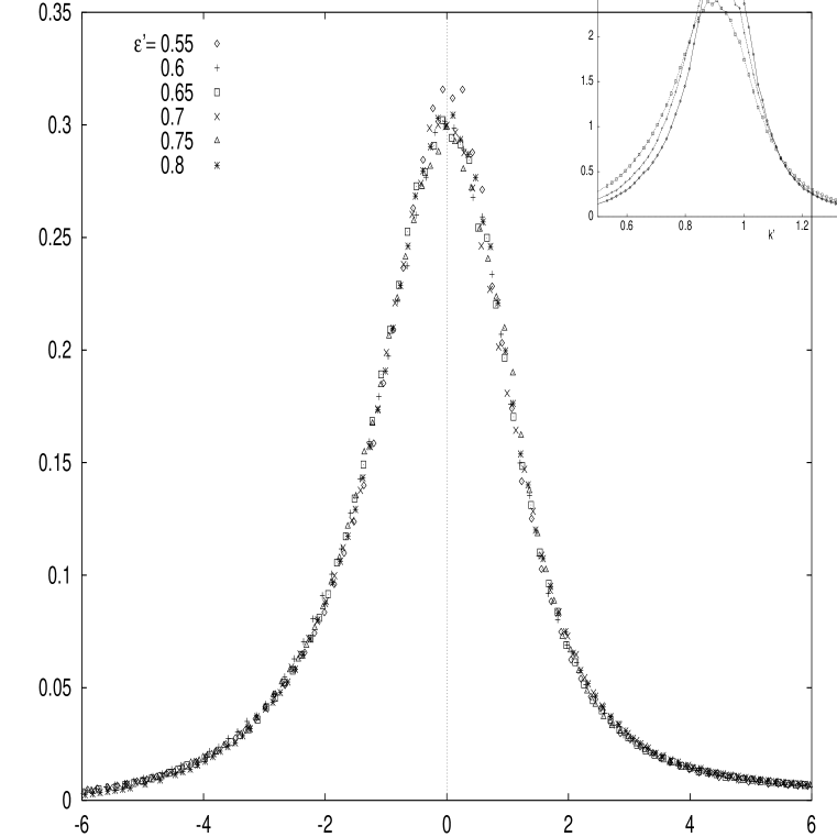
$\frac{k^{\prime}S^{\prime}(k^{\prime})}{\xi_{2}^{\prime}}$ $(k^{\prime}-k_{max}^{\prime})\xi_{2}^{\prime}$

FIG. 2.:

$\xi_{2}k^{3}S(k)$

$k$

(a)
$\xi^{\prime}_{2}k^{\prime 3}S^{\prime}(k^{\prime})$

$k^{\prime}$

(b)

FIG. 3.:

REFERENCES

• [1]
• [2] For a recent review on pattern formation in various systems, see: M. C. Cross and P. C. Hohenberg, Rev. Mod. Phys. 65, 851 (1993).
• [3] G. Ahlers, in 25 Years of Nonequilibrium Statistical Mechanics, edited by J. J. Brey et al. (Springer, New York, 1995), p. 91.
• [4] S. Chandrasekhar, Hydrodynamic and Hydromagnetic Stability (Dover, New York, 1981); P. Manneville, Dissipative Structures and Weak Turbulence (Academic, San Diego, 1990).
• [5] A. Schlüter, D. Lortz, and F. Busse, J. Fluid Mech. 23, 129 (1965); F. H. Busse, Rep. Prog. Phys. 41, 1929 (1978); F. H. Busse and R. M. Clever, in New Trends in Nonlinear Dynamics and Pattern-Forming Phenomena, edited by P. Coullet and P. Huerre (Plenum Press, New York, 1990), p. 37; and references therein.
• [6] F. H. Busse and E. W. Bolton, J. Fluid Mech. 146, 115 (1984); E. W. Bolton and F. H. Busse, ibid 150 487 (1985).
• [7] S. W. Morris, E. Bodenschatz, D. S. Cannell and G. Ahlers, Phys. Rev. Lett. 71, 2026 (1993); Y. Hu, R. E. Ecke and G. Ahlers, ibid 74, 391 (1995).
• [8] M. Assenheimer and V. Steinberg, Phys. Rev. Lett. 70, 3888 (1993); Nature 367, 345 (1994).
• [9] H.-W. Xi, J. D. Gunton and J. Viñals, Phys. Rev. Lett. 71, 2030 (1993).
• [10] M. Bestehorn, M. Fantz, R. Friedrich, and H. Haken, Phys. Lett. A 174, 48 (1993).
• [11] W. Decker, W. Pesch and A. Weber, Phys. Rev. Lett. 73, 648 (1994).
• [12] S. W. Morris, E. Bodenschatz, D. S. Cannell, and G. Ahlers, Physica D 97, 164 (1996).
• [13] R. V. Cakmur, D. A. Egolf, B. B. Plapp, and E. Bodenschatz, patt-sol/9702003.
• [14] M. C. Cross and Y. Tu, Phys. Rev. Lett. 75, 834 (1995).
• [15] H.-W. Xi and J. D. Gunton, Phys. Rev. E 52, 4963 (1995).
• [16] A. Zippelius and E. D. Siggia, Phys. Rev. A 26, 1788 (1982); Phys. Fluids 26, 2905 (1983).
• [17] F. H. Busse, in Advances in Turbulence 2, Edited by H.-H. Fernholz and H. E. Fiedler (Springer-Verlag, Berlin, 1989); F. H. Busse, M. Kropp, and M. Zaks, Physica D 61, 94 (1992).
• [18] H.-W. Xi, X.-J. Li, and J. D. Gunton, Phys. Rev. Lett. 78, 1046 (1997); and [to be submitted].
• [19] L. A. Segel, J. Fluid Mech. 38, 203 (1969); A. C. Newell and J. A. Whitehead, ibid 38, 279 (1969).
• [20] Y. Pomeau and P. Manneville, J. Phys. (Paris) 40, L609 (1979); ibid 42, 1067 (1981); M. C. Cross and A. C. Newell, Physica D 10, 299 (1984); A. C. Newell, T. Passot and M. Souli, J. Fluid Mech. 220, 187 (1990).
• [21] H. S. Greenside, chao-dyn/9612004.
• [22] J. Swift and P. C. Hohenberg, Phys. Rev. A 15, 319 (1977).
• [23] M. C. Cross, Phys. Fluids 23, 1727 (1980); G. Ahlers, M. C. Cross, P. C. Hohenberg, and S. Safran, J. Fluid Mech. 110, 297 (1981).
• [24] E. D. Siggia and A. Zippelius, Phys. Rev. Lett. 47, 835 (1981); M. C. Cross, Phys. Rev. A 27, 490 (1983); P. Mannevill, J. Phys. (Paris) 44, 759 (1983).
• [25] H.-W. Xi, J. Viñals and J. D. Gunton, Phys. Rev. A 46, R4483 (1992); H.-W. Xi, J. D. Gunton and J. Viñals, Phys. Rev. E 47, R2987 (1993); X.-J. Li, H.-W. Xi, and J. D. Gunton, ibid 54, R3105 (1996).
• [26] H. S. Greenside and M. C. Cross, Phys. Rev. A 31, 2492 (1985).
• [27] For detailed discussions on roll-to-SDC transition, see: X.-J. Li, H.-W. Xi, and J. D. Gunton [to be submitted].
• [28] G. Porod, in Small Angle X-ray Scattering, edited by O. Glatter and O. Kratky (Academic, New York, 1982), p. 17.
• [29] For a recent review, see: A. J. Bray, Adv. Phys. 43, 357 (1994).
• [30] With the approximation described in Eq. (1), one may take $g_{m}=-R_{c}[\zeta_{0}(z)w_{0}(z)\partial^{2}w_{0}(z)/\partial z^{2}]_{z}/k_{c}^{4}[w_{0}(z)\theta_{0}(z)]_{z}[\zeta_{0}^{2}(z)]_{z}$ and $c^{2}=-[\zeta_{0}(z)\partial^{2}\zeta_{0}(z)/\partial z^{2}]_{z}/[\zeta_{0}^{2}(z)]_{z}$, where $[\cdots]_{z}$ means the average over the vertical direction. However, we realize that the evaluation of $g_{m}$ depends on further assumptions and, consequently, more accurate expression for $g_{m}$ may exist.
• [31] Many textbooks are available on critical phenomena and critical dynamics. See, for example: S.-K. Ma, Modern Theory of Critical Phenomena (Addison-Wesley, New York, 1994); N. Goldenfeld, Lectures on Phase Transitions and the Renormalization Group (Addison-Wesley, New York, 1992).