Time-periodic phases in populations of nonlinearly coupled oscillators with bimodal frequency distributions

Abstract

The mean field Kuramoto model describing the synchronization of a population of phase oscillators with a bimodal frequency distribution is analyzed (by the method of multiple scales) near regions in its phase diagram corresponding to synchronization to phases with a time periodic order parameter. The richest behavior is found near the tricritical point were the incoherent, stationarily synchronized, “traveling wave” and “standing wave” phases coexist. The behavior near the tricritical point can be extrapolated to the rest of the phase diagram. Direct Brownian simulation of the model confirms our findings.

I Introduction

In recent years mathematical modeling and analysis of synchronization phenomena received increased attention because of its occurrence in quite different fields, such as solid state physics [4, 5, 6], biological systems [7, 8, 9, 10], chemical reactions [11], etc. These phenomena can be modeled in terms of populations of interacting, nonlinearly coupled oscillators as first proposed by Winfree [7]. While the dynamic behavior of a small number of oscillators can be quite rich [12], here we are concerned with synchronization as a collective phenomenon for large populations of interacting oscillators [8].

A simple model put forth by Kuramoto and Sakaguchi [13, 14] (see also [8]), consists of a population of coupled phase oscillators, $\theta_{i}(t)$, having natural frequencies $\omega_{i}$ distributed with a given probability density $g(\omega)$

$$\dot{\theta_{i}}=\omega_{i}+\xi_{i}(t)+\sum_{j=1}^{N}K_{ij}\sin(\theta_{j}-\theta_{i}),\quad\quad i=1,\ldots,N.$$ (1)

Here $\xi_{i}$ are independent white noise processes with expected values

$$\langle\xi_{i}(t)\rangle=0,\ \ \ \langle\xi_{i}(t)\xi_{j}(t^{\prime})\rangle=2D\delta(t-t^{\prime})\,\delta_{ij}.$$ (2)

Thus each oscillator tries to run independently at its own frequency while the coupling tends to synchronize it to all the others. When the coupling is sufficiently weak the oscillators run incoherently whereas beyond a certain threshold collective synchronization appears spontaneously. So far, several particular prescriptions for the matrix $K_{ij}$ have been considered. For instance, $K_{ij}=K>0$ only when $|i-j|=1$, and $K_{ij}=0$ otherwise (next-neighbor coupling) [15]; $K_{ij}=K/N>0$ (mean-field coupling) [13, 11]; hierarchical coupling [16]; random long-range coupling [17, 18, 19] or even state dependent interactions [20]. In the mean-field case, the model (1)-(2) can be written in a convenient form, defining the (complex-valued) order-parameter

$$re^{i\psi}=\frac{1}{N}\sum_{j=1}^{N}e^{i\theta_{j}},$$ (3)

where $r(t)\geq 0$ measures the phase coherence of the oscillators, and $\psi(t)$ measures the average phase. Then eq. (1) reads

$$\dot{\theta_{i}}=\omega_{i}+Kr\sin(\psi-\theta_{i})+\xi_{i}(t),\ \ \ i=1,2,\ldots,N.$$ (4)

In the limit of infinitely many oscillators, $N\rightarrow\infty$, a nonlinear integro-differential equation of the Fokker-Planck type was derived [21, 22] for the one-oscillator probability density, $\rho(\theta,t,\omega)$,

$$\frac{\partial\rho}{\partial t}=D\frac{\partial^{2}\rho}{\partial\theta^{2}}-\frac{\partial}{\partial\theta}(v\rho),$$ (5)

the drift-term being given by

$$v(\theta,t,\omega)=\omega+Krsin(\psi-\theta),$$ (6)

and the order-parameter amplitude by

$$re^{i\psi}=\int_{0}^{2\pi}\!\!\int_{-\infty}^{+\infty}e^{i\theta}\rho(\theta,t,\omega)g(\omega)\,d\theta\,d\omega.$$ (7)

The probability density is required to be $2\pi$-periodic as a function of $\theta$ and normalized according to

$$\int_{0}^{2\pi}\rho(\theta,t,\omega)d\theta=1.$$ (8)

Mean-field models such as those described above were studied, e.g, by Strogatz and Mirollo [22] in case the frequency distribution, $g(\omega)$, has reflection symmetry, $g(-\omega)=g(\omega)$ and it is unimodal [$g(\omega)$ is non-increasing for $\omega>0$]. In [22], the authors showed that for $K$ smaller than a certain value $K_{c}$, the incoherent equiprobability distribution, $\rho_{0}\equiv 1/(2\pi)$, is linearly stable, and linearly unstable for $K>K_{c}$. As $D\to 0+$, the incoherence solution is still unstable for $K>K_{c}$ [$=2/\pi g(0)$ at $D=0$], but it is neutrally stable for $K<K_{c}$: the whole spectrum of the equation linearized about $\rho_{0}$ collapses to the imaginary axis. In [23], the nonlinear stability issue was addressed, and the case of a bimodal frequency distribution was considered [$g(\omega)$ is even and it has maxima at $\omega=\pm\omega_{0}$]. In this case, new bifurcations appear, and bifurcating synchronized states have been asymptotically constructed in the neighborhood of the bifurcation values of the coupling strength. The nonlinear stability properties of such solutions were also studied for the explicit discrete example $g(\omega)={1\over 2}[\delta(\omega-\omega_{0})+\delta(\omega+\omega_{0})]$, cf. [23]. A complete bifurcation study taking into account the symmetry properties of $g(\omega)$ was carried out by Crawford, [24]. Similar results were obtained by Okuda and Kuramoto in the related case of mutual entrainment between populations of coupled oscillators with different frequencies [25]. The main results concerning linear stability of incoherence with a bimodal discrete frequency distribution are summarized in Fig.1 (cf. Fig.1, p.319 in [23]). Also, in Fig.5, p. 327 of [23] a global bifurcation diagram left unresolved the full behavior of the oscillatory branch starting at K=4D.

The purpose of this paper is to complete the investigation started in [23], analyzing in detail (asymptotically) the solution living in the neighborhood of the tricritical point $(K/D=4,\omega_{0}/D=1)$ in the parameter space $(K/D,\omega_{0}/D)$, Fig.1. It turns out that such a task is far from being merely a detail, since technical difficulties are nontrivial at all, and results allow to complete the conjectured diagram in Fig.4 as shown in Fig.5 below. In Section II, a two-time analysis for the Hopf bifurcation, already developed in [23], is revisited; in Section III, a multiscale analysis is performed near the tricritical point, generalizing the asymptotic analysis earlier accomplished in [23]. The corresponding bifurcation equations have been solved recasting the problem into a general formalism due to Dangelmayr and Knobloch [26]. Numerical results designed to confirm the previous findings are presented in Section IV, and these are summarized along with the analytical results in Section V.

II Two-time scale analysis for the Hopf bifurcation

A Linearized problems

Here we revisit certain results given in [23]. In the Hopf analysis conducted there, degeneracy of an eigenvalue of multiplicity two was overlooked, as pointed out by Crawford [24]. We will recall here the relevant points of the linear and nonlinear stability analysis near the line $K=4D$ in Fig. 1 where a Hopf bifurcation from incoherence arises for an even discrete bimodal frequency distribution $g(\omega)$. The linearized eigenvalue problem for this case may be obtained by inserting $\rho=1/(2\pi)+\exp[\lambda t]\,\mu(\theta,\omega)$ in (5) and (6), and then ignoring terms nonlinear in $\mu$:

$$D\frac{\partial^{2}\mu}{\partial\theta^{2}}-\omega\frac{\partial\mu}{\partial\theta}+{K\over 2\pi}\,\mbox{Re}\,e^{-i\theta}\int_{0}^{2\pi}\int_{-\infty}^{+\infty}e^{i\theta^{\prime}}\,\mu(\theta^{\prime},\omega^{\prime})\,g(\omega^{\prime})d\theta^{\prime}d\omega^{\prime}=\lambda\mu,$$ (9)

$$\int_{0}^{2\pi}\mu(\theta,\omega)\,d\theta=0.$$ (10)

It can be shown that there are two eigenvalues $\lambda$, which solve the equation [22]:

$${K\over 2}\,\int_{-\infty}^{+\infty}{g(\nu)\over\lambda+D+i\nu}\,d\nu=1.$$ (11)

They are explicitly given by [23]

$$\lambda_{\pm}=-D+\frac{K}{4}\pm\frac{1}{4}\sqrt{K^{2}-16\omega_{0}^{2}}\,,$$ (12)

when

$$g(\omega)={1\over 2}\,[\delta(\omega-\omega_{0})+\delta(\omega+\omega_{0})]\,.$$ (13)

Fig. 1 is straightforwardly constructed from (12). Above the dashed line, $4\omega_{0}>K$, and the eigenvalues are complex. Each complex eigenvalue is doubly degenerate due to the reflection symmetry of $g(\omega)$ [24]. By direct substitution into (9), it can be checked that

$$\mu_{1}=\frac{e^{i\theta}}{D+\lambda+i\omega}\,,\quad\quad\mu_{2}=\frac{e^{-i\theta}}{D+\lambda-i\omega},$$ (14)

are two linearly independent eigenfunctions corresponding to the same semisimple complex eigenvalue $\lambda$ [24]. They are related by the reflection symmetry $\omega\to-\omega$, $\theta\to-\theta$. When $\lambda$ is real, these eigenfunctions are complex conjugate of each other. The eigenvalue $\lambda$ is no longer semisimple but it still has multiplicity two [24].

B Two-time scale analysis

Let us now recall how to use the method of multiple scales to construct the solution branches which bifurcate from incoherence at $K=4D$, $\omega_{0}>D$ [23]. We define a small positive parameter $\varepsilon$ which measures the departure from the critical value $K_{c}=4D$ by

$$K=K_{c}+\varepsilon^{2}K_{2},\quad\quad 0<\varepsilon\ll 1.$$ (15)

$K_{2}=\pm 1$ has to be determined later according to the direction of the bifurcating branch and the scaling (15) will be justified later. The probability density $\rho(\theta,t,\omega;\epsilon)$ will be sought for according to the Ansatz [23]:

$$\rho(\theta,t;\omega;\varepsilon)=\frac{1}{2\pi}\exp\left\{\sum_{j=1}^{3}\varepsilon^{j}\sigma_{j}(\theta,t,\tau)+O(\varepsilon^{4})\right\}\,$$ (16)

$$\tau=(K-K_{c})t=\varepsilon^{2}K_{2}t.$$ (17)

The rationale behind (16) is as follows. First of all, near $K=K_{c}$, small disturbances from incoherence decay or grow according to the values of the factor

$$\exp[\lambda(K)t]\sim\exp\left[\mbox{Re}{\partial\lambda(K_{c})\over\partial K}(K-K_{c})t+i\,\mbox{Im}\lambda(K_{c})t\right]\,.$$ (18)

Here $\lambda(K)$ is given by (12) with $K$ given by (15) and $\omega_{0}>D$. Hence $\lambda(K)\sim\pm i\Omega+\varepsilon^{2}K_{2}(1\mp iD/\Omega)/4$, where $\Omega=\sqrt{\omega_{0}^{2}-D^{2}}$. This explains the appearance of the two distinguished time scales $t$ and $\tau$. The exponential Ansatz (16) was introduced in [21] motivated by the failure of the usual expansion of $\rho$ in power series of $\varepsilon$ for the particular model considered there. For that model, an algebraic Ansatz yields a vertical bifurcating branch to all orders in $\varepsilon$. In other models where the unknown $\rho$ is everywhere non-negative, such an exponential Ansatz yields an asymptotic expansion (in $\varepsilon$) with larger domain of validity than a purely algebraic Ansatz [27].

Inserting (16) and (17) into the governing equations (5)-(8), we obtain the hierarchy (3.5a)-(3.7b) of [23]:

$${\cal L}\sigma_{1}\equiv(\partial_{t}-D\partial_{\theta}^{2}+\omega\partial_{\theta})\sigma_{1}-K_{c}\mbox{Re}\,e^{-i\theta}\langle e^{i\theta^{\prime}},\sigma_{1}\rangle=0,$$ (19)

(20)

$$\int_{0}^{2\pi}\sigma_{1}d\theta=0,$$ (21)

$${\cal L}\left(\sigma_{2}+\frac{\sigma_{1}^{2}}{2}\right)=-K_{c}\partial_{\theta}\left\{\sigma_{1}\mbox{Im}\ e^{-i\theta}\langle e^{i\theta^{\prime}},\sigma_{1}\rangle\right\},$$ (22)

(23)

$$\int_{0}^{2\pi}\left(\sigma_{2}+\frac{\sigma_{1}^{2}}{2}\right)d\theta=0,$$ (24)

$${\cal L}\left(\sigma_{3}+\sigma_{1}\sigma_{2}+\frac{\sigma_{1}^{2}}{6}\right)=-K_{c}\,\partial_{\theta}\left\{\left(\sigma_{2}+\frac{\sigma_{1}^{2}}{2}\right)\,\mbox{Im}\ e^{-i\theta}\langle e^{i\theta^{\prime}},\sigma_{1}\rangle\right.\quad\quad$$ (25)

$$\left.+\sigma_{1}\mbox{Im}\ e^{-i\theta}\langle e^{i\theta^{\prime}},\sigma_{2}+\frac{\sigma_{1}^{2}}{2}\rangle\right\}-K_{2}[\partial_{\tau}\sigma_{1}+\partial_{\theta}\mbox{Im}\ e^{-i\theta}\langle e^{-i\theta^{\prime}},\sigma_{1}\rangle],$$ (26)

(27)

$$\int_{0}^{2\pi}\left(\sigma_{3}+\sigma_{1}\sigma_{2}+\frac{\sigma_{1}^{2}}{6}\right)d\theta=0.$$ (28)

Here we have defined the following scalar product [23]

$$\langle\alpha(\theta,\omega),\beta(\theta,\omega)\rangle=\frac{1}{2\pi}\int_{0}^{2\pi}\int_{-\infty}^{+\infty}\alpha(\theta,\omega)\beta(\theta,\omega)g(\omega)d\omega d\theta.$$ (29)

The solution of the homogeneous linear equation (20) is a linear combination of $\mu_{l}e^{i\Omega t}$, $l=1,2$ and the complex conjugates of these terms [the $\mu_{l}$ are given by (14)]:

$$\sigma_{1}=\frac{A_{+}(\tau)}{D+i(\Omega+\omega)}e^{i(\Omega t+\theta)}+cc+\frac{A_{-}(\tau)}{D+i(\Omega-\omega)}e^{i(\Omega t-\theta)}+cc,$$ (30)

where $\Omega^{2}=\omega_{0}^{2}-D^{2}$ and $cc$ denotes the complex conjugate of the preceding term (in [23] there was $A_{-}\equiv 0$, $A_{+}\equiv A$. Thus two terms were missing). This value of $\sigma_{1}$ has also zero mean, as a function of $\theta$. Insertion of this equation in (23) and (27) yields

$${\cal L}(\sigma_{2}+\frac{\sigma_{1}^{2}}{2})=2e^{2i\Omega t}\left(\frac{A_{+}^{2}e^{2i\theta}}{D+i(\Omega+\omega)}+\frac{A_{-}^{2}e^{-2i\theta}}{D+i(\Omega-\omega)}\right)+cc$$ (31)

$$+4e^{2i\theta}A_{+}\overline{A}_{-}\frac{D+i\omega}{(D+i\omega)^{2}+\Omega^{2}}+cc,$$ (32)

from which

$$\sigma_{2}+\frac{\sigma_{1}^{2}}{2}=\frac{2(D+i\omega)A_{+}\overline{A}_{-}}{(2D+i\omega)[(D+i\omega)^{2}+\Omega^{2}]}e^{2i\theta}+cc$$ (33)

$$+\frac{A_{+}^{2}e^{2i(\Omega t+\theta)}}{[D+i(\Omega+\omega)][2D+i(\Omega+\omega)]}+cc$$ (34)

$$+\frac{A_{-}^{2}e^{2i(\Omega t-\theta)}}{[D+i(\Omega-\omega)][2D+i(\Omega-\omega)]}+cc,$$ (35)

which has also zero mean, as required. After lengthy but rather elementary calculations to evaluate the right-hand side of (27), this equation takes on the form

$${\cal L}(\sigma_{3}+\sigma_{1}\sigma_{2}+\frac{\sigma_{1}^{3}}{6})=Q_{+}(\tau,\omega)e^{i(\Omega t+\theta)}+cc+Q_{-}(\tau,\omega)e^{i(\Omega t-\theta)}+cc,$$ (36)

where only the terms that may be resonant have been kept. It is natural to look for a solution of the form

$$\sigma_{3}+\sigma_{1}\sigma_{2}+\frac{\sigma_{1}^{3}}{6}=P_{+}e^{i(\Omega t+\theta)}+cc+P_{-}e^{i(\Omega t-\theta)}+cc.$$ (37)

We determine $P_{\pm}$ by substitution of (37) into (36),

$$[D+i(\Omega\pm\omega)]P_{\pm}-{K_{c}\over 2}\,\langle 1,P_{\pm}\rangle=Q_{\pm}.$$ (38)

Then we can solve for $P_{\pm}$:

$$P_{\pm}={K_{c}\langle 1,P_{\pm}\rangle\over 2[D+i(\Omega\pm\omega)]}+{Q_{\pm}\over D+i(\Omega\pm\omega)}\,.$$ (39)

¿From (11) and the reflection symmetry of $g(\omega)$, we know that ${1\over 2}K_{c}\langle 1,1/[D+i(\Omega\pm\omega)]\rangle=1$, so that the scalar product of 1 with (39) produces the following non-resonance conditions:

$$\langle\frac{Q_{+}}{D+i(\Omega+\omega)}\rangle=0$$ (40)

$$\langle\frac{Q_{-}}{D+i(\Omega-\omega)}\rangle=0,$$ (41)

where we set

$$\langle\alpha(\omega)\rangle=\int_{-\infty}^{+\infty}\alpha(\omega)g(\omega)d\omega.$$ (42)

The zero mean condition is also satisfied automatically. Some more tedious calculations lead finally to two nonlinear coupled ordinary differential equations for $A_{+}(\tau),A_{-}(\tau)$:

$$\dot{A}_{+}=\alpha A_{+}-(\beta|A_{-}|^{2}+\gamma|A_{+}|^{2})\,A_{+},$$ (43)

(44)

$$\dot{A}_{-}=\alpha A_{-}-(\beta|A_{+}|^{2}+\gamma|A_{-}|^{2})\,A_{-},$$ (45)

where   $\dot{}=d/d\tau$, and

$$\alpha=\frac{1}{4}-\frac{iD}{4\Omega}\,,$$ (46)

$$\beta=\frac{D+i{D^{2}+\omega_{0}^{2}\over\Omega}}{K_{2}\,(4D^{2}+\omega_{0}^{2})}\,,$$ (47)

$$\gamma=\frac{2(3D^{2}+4\omega_{0}^{2})+iD\,{3D^{2}+2\omega_{0}^{2}\over\Omega}}{DK_{2}\,(9D^{2}+16\omega_{0}^{2})}\,.$$ (48)

This result favorably agrees with that of  [23] when we set $A_{+}\equiv A,\,A_{-}\equiv 0$. The needed stability analysis is, consequently, a little more involved than that in  [23]. Let us define the new variables

$$u=|A_{+}|^{2}+|A_{-}|^{2},\ \ \ v=|A_{+}|^{2}-|A_{-}|^{2}.$$ (49)

By using (44), we obtain the following system for $u$ and $v$:

$$\dot{u}=2\ \mbox{Re}\ \alpha\ u-\mbox{Re}(\gamma+\beta)\ u^{2}-\mbox{Re}(\gamma-\beta)\ v^{2},$$

$$\dot{v}=2\ \mbox{Re}\ \alpha\ v-2\ \mbox{Re}\ \gamma\ uv.$$ (50)

Clearly, $u=v$ or $u=-v$ correspond to traveling wave (TW) solutions, while $v\equiv 0$ corresponds to standing wave (SW) solutions. The phase portrait corresponding to $\alpha$, $\beta$ and $\gamma$ of (44) is easily found (see Fig. 2), and the explicit solutions are (up to, possibly, a constant phase shift)

$$A_{+}(\tau)=\sqrt{\frac{\mbox{Re}\ \alpha}{\mbox{Re}\ \gamma}}\ e^{i\mu\tau},\ \ A_{-}(\tau)\equiv 0,\ \ \ \mu=\mbox{Im}\ \alpha-\frac{\mbox{Im}\ \gamma}{\mbox{Re}\ \gamma}\,\mbox{Re}\ \alpha$$ (51)

(or $A_{+}(\tau)\equiv 0$ and $A_{-}(\tau)$ as $A_{+}(\tau)$ above) in case of TW solutions, and

$$A_{+}(\tau)=A_{-}(\tau)=\sqrt{\frac{\mbox{Re}\ \alpha}{\mbox{Re}\ (\gamma+\beta)}}\ e^{i\nu\tau},\ \ \ \nu=\mbox{Im}\ \alpha-\frac{\mbox{Im}\ (\gamma+\beta)}{\mbox{Re}\ (\gamma+\beta)}\,\mbox{Re}\ \alpha$$ (52)

in case of SW solutions. Notice that both SW and TW bifurcate supercritically with $\|r_{SW}\|/r_{TW}>1$, as indicated in Fig. 3: Re$(\beta+\gamma)$ and Re$\gamma$ are both positive when $K_{2}=1$; whereas the square roots in (51) and (52) become pure imaginary if $K_{2}=-1$. This indicates that the bifurcating branches cannot be subcritical. From the phase portrait corresponding to (44), it follows that the SWs are always globally stable, while the TWs are unstable. Such result was pointed out in [24], following completely different methods, while in [23] the analysis was restricted to the case $u^{2}=v^{2}$, and thus the TWs were erroneously found to be stable.

III Multiscale analysis near the tricritical point

Asymptotic analysis near the tricritical point, $P=(K/D=4,\omega_{0}/D=1)$ in Fig.1, leads to the introduction of a third time-scale. In fact, near such a point,

$$K=K_{c}+K_{2}\varepsilon^{2}+O(\varepsilon^{3}),\ \ \ \omega_{0}=\omega_{0c}+\omega_{2}\varepsilon^{2}+O(\varepsilon^{3})\ \ \ (K_{c}=4D,\ \omega_{0c}=D),$$ (53)

and

$$\lambda_{\pm}=-D+\frac{K}{4}\pm\frac{1}{4}\sqrt{K^{2}-16\omega_{0}^{2}}\approx\frac{K_{2}}{4}\varepsilon^{2}\pm\frac{\varepsilon}{4}\sqrt{8D(K_{2}-4\omega_{2})}.$$ (54)

This shows that, besides the basic time-scale (which is denoted by $t$), and the slow time $\tau=\varepsilon^{2}t$ (as in [23]), an intermediate scale, say $T=\varepsilon t$, appears. Compare

$$e^{\lambda_{\pm}t}\sim\exp\left\{\frac{K_{2}}{4}\tau\pm\frac{\sqrt{8D(K_{2}-4\omega_{2})}}{4}T\right\}\,$$ (55)

with (18) above. Consequently, the slightly different Ansatz

$$\rho(\theta,t;\omega;\varepsilon)=\frac{1}{2\pi}\exp\left\{\sum_{j=1}^{4}\varepsilon^{j}\sigma_{j}(\theta,t,T,\tau)+O(\varepsilon^{5})\right\}\,$$ (56)

is needed. Inserting (53) and (56) into the governing equations (5)-(8) leads to the hierarchy below, instead of (20)-(27):

$${\cal L}\sigma_{1}=(\partial_{t}-D\partial_{\theta}^{2}+\omega\partial_{\theta})\sigma_{1}+4D\partial_{\theta}\left\{\mbox{Im}\ e^{-i\theta}\langle e^{i\theta^{\prime}},\sigma_{1}\rangle\right\}=0,$$ (57)

(58)

$$\int_{0}^{2\pi}\sigma_{1}d\theta=0,$$ (59)

$${\cal L}\left(\sigma_{2}+\frac{\sigma_{1}^{2}}{2}\right)=-4D\partial_{\theta}\left\{\sigma_{1}\mbox{Im}\ e^{-i\theta}\langle e^{i\theta^{\prime}},\sigma_{1}\rangle\right\}-\partial_{T}\sigma_{1},$$ (60)

(61)

$$\int_{0}^{2\pi}\left(\sigma_{2}+\frac{\sigma_{1}^{2}}{2}\right)d\theta=0,$$ (62)

$${\cal L}\left(\sigma_{3}+\sigma_{1}\sigma_{2}+\frac{\sigma_{1}^{2}}{6}\right)=-4D\,\partial_{\theta}\left\{\sigma_{1}\mbox{Im}\ e^{-i\theta}\langle e^{i\theta^{\prime}},\sigma_{2}+\frac{\sigma_{1}^{2}}{2}\rangle+\left(\sigma_{2}+\frac{\sigma_{1}^{2}}{2}\right)\mbox{Im}\ e^{-i\theta}\langle e^{i\theta^{\prime}},\sigma_{1}\rangle\right.$$ (63)

$$\left.+\omega_{2}\,\mbox{Im}\ e^{-i\theta}\langle e^{i\theta^{\prime}},\sigma_{1}\rangle^{\prime}\right\}-K_{2}\partial_{\theta}\mbox{Im}\ e^{-i\theta}\langle e^{-i\theta^{\prime}},\sigma_{1}\rangle-\partial_{\tau}\sigma_{1}-\partial_{T}\left(\sigma_{2}+\frac{\sigma_{1}^{2}}{2}\right),$$ (64)

(65)

$$\int_{0}^{2\pi}\left(\sigma_{3}+\sigma_{1}\sigma_{2}+\frac{\sigma_{1}^{2}}{6}\right)d\theta=0,$$ (66)

$${\cal L}\left(\sigma_{4}+\sigma_{1}\sigma_{3}+\frac{\sigma_{2}^{2}}{2}+\frac{\sigma_{1}^{2}\sigma_{2}}{2}+\frac{\sigma_{1}^{4}}{4!}\right)=-4D\partial_{\theta}\left\{\sigma_{1}\mbox{Im}\ e^{-i\theta}\langle e^{-i\theta^{\prime}},\sigma_{3}+\sigma_{1}\sigma_{2}+\frac{\sigma_{1}^{3}}{6}\rangle\right.$$ (67)

$$\left.+\left(\sigma_{3}+\sigma_{1}\sigma_{2}+\frac{\sigma_{1}^{3}}{6}\right)\mbox{Im}\ e^{-i\theta}\langle e^{i\theta^{\prime}},\sigma_{1}\rangle+\omega_{2}\mbox{Im}\ e^{-i\theta}\langle e^{i\theta^{\prime}},\sigma_{2}+\frac{\sigma_{1}^{2}}{2}\rangle^{\prime}\right.$$ (68)

$$\left.+\omega_{2}\sigma_{1}\mbox{Im}\ e^{i\theta}\langle e^{i\theta^{\prime}},\sigma_{1}\rangle^{\prime}+\left(\sigma_{2}+\frac{\sigma_{1}^{2}}{2}\right)\mbox{Im}\ e^{-i\theta}\langle e^{i\theta^{\prime}},\sigma_{2}+\frac{\sigma_{1}^{2}}{2}\rangle\right\}$$ (69)

$$-K_{2}\,\partial_{\theta}\left\{\mbox{Im}\ e^{-i\theta}\langle e^{i\theta^{\prime}},\sigma_{2}+\frac{\sigma_{1}^{2}}{2}\rangle+\sigma_{1}\mbox{Im}\ e^{-i\theta}\langle e^{i\theta^{\prime}},\sigma_{1}\rangle\right\}$$ (70)

$$-\partial_{\tau}\left(\sigma_{2}+\frac{\sigma_{1}^{2}}{2}\right)-\partial_{T}\left(\sigma_{3}+\sigma_{1}\sigma_{2}+\frac{\sigma_{1}^{2}}{2}\right),$$ (71)

(72)

$$\int_{0}^{2\pi}\left(\sigma_{4}+\sigma_{1}\sigma_{3}+\frac{\sigma_{2}^{2}}{2}+\frac{\sigma_{1}^{2}\sigma_{2}}{2}+\frac{\sigma_{1}^{4}}{4!}\right)d\theta=0.$$ (73)

Here

$$\langle\alpha(\theta,\omega),\beta(\theta,\omega)\rangle^{\prime}=\frac{1}{2\pi}\int_{0}^{2\pi}\int_{-\infty}^{+\infty}\alpha(\theta,\omega)\beta(\theta,\omega)g_{\omega_{0}}^{\prime}(\omega)d\theta d\omega,$$ (74)

where

$$g_{\omega_{0}}^{\prime}(\omega)=\frac{1}{2}\left[\delta^{\prime}(\omega+\omega_{0})-\delta^{\prime}(\omega-\omega_{0})\right]\ \ \ \ \ (\omega_{0}=\omega_{0c}=D).$$ (75)

The solution of the homogeneous equation (58) for $\sigma_{1}$ is immediately found [$\Omega=0$ in (30)]:

$$\sigma_{1}=\frac{A(T,\tau)}{D+i\omega}e^{i\theta}+cc,$$ (76)

plus terms which decay exponentially on the fast time scale, $t$, and which we will systematically omit. Inserting this into equation (61), we obtain

$${\cal L}\left(\sigma_{2}+\frac{\sigma_{1}^{2}}{2}\right)=-\frac{A_{T}}{D+i\omega}e^{i\theta}+cc+\frac{2A^{2}}{D+i\omega}e^{2i\theta}+cc,$$ (77)

wherefrom

$$\sigma_{2}+\frac{\sigma_{1}^{2}}{2}=-\frac{A_{T}}{(D+i\omega)^{2}}e^{i\theta}+cc+\frac{A^{2}}{(D+i\omega)(2D+i\omega)}e^{2i\theta}+cc+\frac{B(T,\tau)}{D+i\omega}e^{i\theta}+cc,$$ (78)

and hence $\sigma_{2}$. Note that the term containing $B(T,\tau)$ is the solution of the homogeneous equation associated to $\cal L$ [cf. (76)]. Proceeding in a similar way, we obtain

$$\sigma_{3}+\sigma_{1}\sigma_{2}+\frac{\sigma_{1}^{3}}{6}=\left[\frac{K_{2}-4\omega_{2}}{4D(D+i\omega)}A-\frac{B_{T}}{(D+i\omega)^{2}}+\frac{A_{TT}}{(D+i\omega)^{3}}-\frac{A_{\tau}}{(D+i\omega)^{2}}+\frac{C(T,\tau)}{D+i\omega}\right.$$ (79)

$$\left.-\frac{A|A|^{2}}{(D+i\omega)^{2}(2D+i\omega)}\right]\,e^{i\theta}+cc+\frac{2AB-AA_{T}\left(\frac{1}{D+i\omega}+\frac{1}{2D+i\omega}\right)}{(D+i\omega)(2D+i\omega)}e^{2i\theta}$$ (80)

$$+cc+\frac{A^{3}e^{3i\theta}}{(D+i\omega)(2D+i\omega)(3D+i\omega)}+cc,$$ (81)

where $C\equiv C(T,\tau)$ has a meaning similar to that of $A$ and $B$. ¿From this we obtain $\sigma_{3}$, and finally, from (72), $\sigma_{4}$. To obtain the leading order approximation, we only need to determine $A(T,\tau)$. Now, (81) holds provided that the nonresonance condition (needed to remove secular terms)

$$\langle\frac{1}{D+i\omega},P(\omega,T,\tau)\rangle=0$$ (82)

holds, where $P(\omega,T,\tau)$ denotes the coefficient of $e^{i\theta}$ on the right-hand side of (65). Equation (82) turns out to be the “complex Duffing equation”

$$A_{TT}-\frac{D}{2}(K_{2}-4\omega_{2})A-\frac{2}{5}|A|^{2}A=0.$$ (83)

Such equation, however, is not sufficient to determine $A$, in view of the two time scales on which $A$ depends. The nonresonance condition for $\sigma_{4}$, i.e. an equation like that in (82) where $P(\omega,T,\tau)$ now denotes the coefficient of $e^{i\vartheta}$ on the right-hand side of (72), is the “linearized inhomogeneous Duffing equation”

$$B_{TT}-\frac{D}{2}(K_{2}-4\omega_{2})B-\frac{2}{5}(A^{2}\overline{B}+2|A|^{2}B)=-2A_{T\tau}+\frac{K_{2}}{2}A_{T}$$ (84)

$$-\frac{\left(|A|^{2}A\right)_{T}}{5D}-\frac{23}{25D}|A|^{2}A_{T},$$ (85)

where an overbar denotes taking the complex conjugate.

Equations (83) and (85) could be analyzed directly, e.g. by extending the Kuzmak-Luke method (see [28], Section 4.4), to find the bifurcating solutions in the vicinity of the tricritical point and their stability. However, we can take advantage from the already existing, rather comprehensive theory of amplitude equations for systems invariant under the $O(2)$ group of rotations ($\theta\to\theta+\varphi$) and reflections ($\theta\to-\theta$, $\omega\to-\omega$) developed by Dangelmayr and Knobloch in [26]. Our nonlinear Fokker-Planck problem has this symmetry, therefore the normal form near the tricritical point (a Takens-Bogdanov bifurcation) should be the same one that Dangelmayr and Knobloch studied. Equations (83) and (85) in fact can be used to reconstruct the scaled “normal form”:

$$U^{\prime\prime}-\varepsilon[c_{1}U^{\prime}+c_{2}(\overline{U}U^{\prime}+U\overline{U}^{\prime})\,U+c_{3}|U|^{2}U^{\prime}]-(c_{4}+c_{5}|U|^{2})U=O(\varepsilon^{2}),\ \ \ \ ^{\prime}=\frac{d}{dT}\,,$$ (86)

studied by Dangelmayr and Knobloch in [26] [cf. their equations (3.3), p. 2480]; recall that $T=\varepsilon t$ is the slow scale. Setting

$$U=A(T,\tau)+\varepsilon B(T,\tau)\equiv A(T,\varepsilon T)+\varepsilon B(T,\varepsilon T)$$ (87)

in (86), we obtain equations for $A$ and $B$ which are of the same form as (83) and (85). We can then identify the parameters termed $\mu$, $\nu$, $A$, $C$, $D$ in [26], and thus $M=2C+D$ there, with our quantities

$$\frac{D}{2}(K_{2}-4\omega_{2}),\ \ \ \frac{K_{2}}{2},\ \ \ \frac{2}{5},\ \ \ -\frac{1}{5D},\ \ \ -\frac{28}{25D},\ \ \ \mbox{and}\ \ -\frac{38}{25D},$$ (88)

respectively. With these identifications, Equation (86) becomes

$$U_{TT}-\frac{D}{2}(K_{2}-4\omega_{2})U-\frac{2}{5}|U|^{2}U=\varepsilon\,\left(\frac{K_{2}}{2}U_{T}-\frac{23}{25D}|U|^{2}U_{T}-\frac{1}{5D}(|U|^{2}U)_{T}\right)+O(\varepsilon^{2}).$$ (89)

Note that $-2A_{T\tau}\varepsilon=O(\varepsilon^{2})$. The general analysis developed in [26] for equation (86) can be used for the present case, equation (89) [cf. [26], equation (3.3)]. We make the substitution

$$U(T;\varepsilon)=R(T;\varepsilon)e^{i\phi(T;\varepsilon)}$$ (90)

in equation (89), separate real and imaginary parts, and then obtain the perturbed Hamiltonian system

$$R_{TT}+\frac{\partial V}{\partial R}=\varepsilon\left(\frac{K_{2}}{2}-\frac{38}{25D}R^{2}\right)R_{T},$$ (91)

(92)

$$L_{T}=\varepsilon\left(\frac{K_{2}}{2}-\frac{28}{25D}R^{2}\right)L,$$ (93)

where

$$L=R^{2}\phi_{T}$$ (94)

is the angular momentum, and

$$V\equiv V(R)=\frac{L^{2}}{2R^{2}}-\frac{D}{4}\left(K_{2}-4\omega_{2}\right)R^{2}-\frac{R^{4}}{10}$$ (95)

is the potential. This system may have the following special solutions (whose stability properties are also pointed out here):

• The trivial solution, $L=0$, $R=0$, which corresponds to the incoherent probability density, $\rho=1/2\pi$. Such solution is stable for $K_{2}<0$ if $\omega_{2}>0$ and for $(K_{2}-4\omega_{2})<0$ if $\omega_{2}<0$.

• The steady-states (SS), $L=0$, $R=R_{0}=\sqrt{5D\left(\omega_{2}-\frac{K_{2}}{4}\right)}>0$, which exists provided that $\omega_{2}>K_{2}/4$. This solution is always unstable.

• The traveling waves (TW), $L=L_{0}=R_{0}^{2}\sqrt{2D\left(\omega_{2}-\frac{19}{56}K_{2}\right)}>0$, $R=R_{0}=\frac{5}{2}\sqrt{\frac{DK_{2}}{14}}>0$, which exist provided that $K_{2}>0$ and $\omega_{2}>19K_{2}/56$; these solutions bifurcate from the trivial solution at $K_{2}=\omega_{2}=0$. When $\omega_{2}=19K_{2}/56$, the branch of TWs merges with the steady-state solution branch. This solution is always unstable.

• The standing waves (SW), $L=0$, $R=R(T)$ periodic. Such solutions have been found explicitly in Section 5.1 of [26]. The SWs branch off the trivial solution at $K_{2}=\omega_{2}=0$, exist for $\omega_{2}>11K_{2}/19>0$, and terminate by merging with a homoclinic orbit of the steady-state $(ii)$ on the line $\omega_{2}=11K_{2}/19$ [see equation (5.8) of [26]]. This solution is always stable.

All these results are depicted in Fig. 3 below, which corresponds to Fig. 4, IV-, in the general classification (stability diagrams) reported in [26], p.266.

In Fig. 4 below, the bifurcation diagram relevant to the present problem with $\omega_{2}>0$ is given (cf. Fig.5, IV-, in [26], p.267).

Note that the modulated wave solutions (in the terminology of [26]), i.e. with both $L$ and $R$ periodic functions, in general with different periods, do not appear in the problem studied in the present paper.

In closing, observe that, to the leading order, equation (56) yields

$$\rho(\theta,t;\omega;\varepsilon)\sim\frac{1}{2\pi}\left[1+\varepsilon\frac{Re^{i(\phi+\theta)}}{D+i\omega}+cc\right],$$ (96)

and hence, from (7),

$$re^{i\psi}\sim\varepsilon\frac{R}{2D}e^{-i\phi}.$$ (97)

It follows that

$$r\sim\varepsilon\frac{R}{2D},\qquad\psi\sim-\phi,$$ (98)

which shows that, essentially, the solution $U(T;\varepsilon)$ to equation (89) coincides with the conjugate of the complex order parameter [defined by (7)]. For this reason, in Fig. 4 the ordinate can be either $R$ or $r$. In Fig. 5, we depicted the global bifurcation diagram which completes the analogous one given in [23], cf. Fig. 5 there.

IV Numerical results

The goal of this section is to give numerical evidence of the theoretical results obtained thus far. To perform this task, we have integrated the stochastic Eq. (4) by a first-order Euler method with a time step $\Delta t=0.005$. In all our simulations a population of $N=50,000$ has been chosen, which is large enough to neglect finite-size effects.

The interesting region in the space of parameters is located above the tricritical point $(K/D=4,\omega_{0}/D=1)$. To explore this region and without loss of generality, we have kept fixed the strength of the noise to $D=1$. Then we have set $\omega_{0}=2$, and we have swept the phase diagram by moving the coupling constant, $K$, thereby finding different behavior according to the results of the previous sections. Consistently with the figures depicted above, we have considered only values $K>4$, for which the incoherent solution $\rho\equiv 1/2\pi$ is unstable. For these values of $K$, the (partially) synchronized SW states bifurcate supercritically and are stable until the SW branch disappears. In this section we define the order parameter (3) or (7) in such a way that $r(t)\in[-1,1]$ and that the phase does not experiences jumps as it increases past odd integer multiples of $\pi$. Then the order parameter which we should use to compare with the results of previous Sections is $|r(t)|\geq 0$.

Let start the discussion considering $K=5.2$ . In Fig. 6, we can see that, after a short transient, the order parameter $|r(t)|$ reaches a stable state characterized by time-periodic oscillations of large amplitude. Clearly, this value of the coupling constant belongs to the domain of the SW solution. This periodic behavior is found as soon as $K$ becomes larger than 4, but near the critical point the frequency of the oscillations is very high (recall that $\omega_{0}=2$) and their amplitude quite small. This is why we do not depict such a behavior in any of the figures. Moreover, when $K=5.2$, the Fourier transform of the order parameter exhibits a large peak at a nonzero frequency, which corresponds to a relaxation oscillation. This peak slowly fades out as $K$ decreases down towards $K=4$ (near the bifurcation point the oscillation becomes sinusoidal).

The opposite behavior is found for larger values of $K$. In comparison with the last figure now the amplitude of the oscillations increases while the frequency decreases in a nontrivial way with the coupling constant as we can see in Fig. 7 for $K=6$. The system still remains in the domain where the standing waves are stable.

According to the theory, the SW solution should merge with the SS solution for values of $K$ large enough. Indeed, this is what we observe in Fig. 8. In this case for $K=7$ the order parameter grows exponentially fast from the initial incoherent solution to the time-independent partially synchronized stationary state. The conjectured global bifurcation diagram of Fig. 5 suggests that there may be a region where the SW and the partially synchronized stationary solution are both stable. In order to detect the presence of bistability, it is more convenient to use a deterministic numerical method to solve the nonlinear Fokker-Planck equation. In fact, the Monte Carlo simulation averages over realizations of the noise. Then different realizations may go to different stable solutions in the bistability region, unless we are rather careful choosing convenient initial conditions within the basin of attraction of one solution, and a small enough time step. Then we need an enormous amount of computing time for a Monte Carlo simulation to distinguish the attractor with smaller basin of attraction in the bistability region. Thus we have used deterministic numerical simulations (finite differences) of the nonlinear Fokker-Planck equation to obtain the results reported below, although we have checked that costly Monte Carlo simulations also yield the same results in several points of the bifurcation diagram. A direct numerical simulation of the nonlinear Fokker-Planck equation by finite differences shows that for sufficiently large $\omega_{0}$ the region of bistability disappears. At $\omega_{0}=1.5$ we have found a narrow region of bistability between SW and SS solutions which is illustrated in Fig. 9. Fig. 9(a) shows that different initial data evolve either to the SW or to the upper SS solution for $K=4.95$. Fig. 9(b) illustrates the abrupt transition from a SW solution to the upper SS solution when $K$ changes from 4.9597 to 4.9598. When $\omega_{0}$ is larger, $\omega_{0}=2$ as in Fig. 10, direct simulations show a smooth transition from SW to SS. This may correspond to having the turning point $K_{1}$ of Fig. 5 close to the end point of the SW branch.

V Summary

We have used the method of multiple scales to study synchronization to oscillatory phases in the mean-field Kuramoto model with a bimodal frequency distribution. Near the Hopf bifurcation points our method recovers Crawford’s results: solution branches of stable standing wavΠes (SW) and unstable traveling waves (TW) issue supercritically from the incoherent (non-synchronized) state. Near the tricritical point (where a line of Hopf bifurcations and a line of partially-synchronized stationary states coalesce) our multiple scale method recovers the normal form for symmetric Takens-Bogdanov bifurcations studied by Dangelmayr and Knobloch. This study allows us to establish that the bifurcating branches given by the local analysis of Section II end as infinite-period bifurcation solutions. The unstable TW branch terminates on the SS branch, whereas the SW branch collides with the homoclinic loop of the SS branch in a global bifurcation of finite amplitude. All results obtained in Sections II and III above agree quantitatively, as it can be shown by asymptotic matching (see Appendix). Furthermore, there may be an interval of parameter values where SW and partially-synchronized stationary solutions are both stable. Brownian and direct finite-difference simulations (Section IV) confirm these results.

VI ACKNOWLEDGMENTS

We are indebted to J. A. Acebrón for drawing figures 1 to 5, 9 and 10 and performing direct numerical simulations of the nonlinear Fokker-Planck equation. We acknowledge financial support from the the Spanish DGICYT through grant PB95-0296, from the Italian Gruppo Nazionale di Fisica Matematica GNFM-CNR, and the EC Human Capital and Mobility Programme under contract ERBCHRXCT930413.

Appendix

The bifurcation diagrams in Sections II and III agree in the sense that the corresponding solutions match asymptotically on some overlap domain. For instance, in case of TW solutions, $A_{+}\neq 0$, $A_{-}\equiv 0$, one obtains from (44)

$$A_{+}e^{i\Omega t}\sim R_{0}\exp\left\{i\Omega t-i\frac{\tau}{\Omega}\left(\frac{D}{4}+\frac{R_{0}^{2}}{5K_{2}}\right)\right\}\sim R_{0}\exp\left\{iT\left[\sqrt{2D\omega_{2}}-\frac{K_{2}}{\sqrt{2D\omega_{2}}}\left(\frac{D}{4}+\frac{R_{0}^{2}}{5K_{2}}\right)\right]\right\},$$ (A.1)

where $R_{0}$ is a constant to be found by asymptotic matching, and $\tau D/\Omega\sim K_{2}T\sqrt{{D\over 2\omega_{2}}}=O(1)$, $K_{2}>0$ fixed, as $\omega_{2}\to 0$ from above. On the other hand, near the tricritical point, it is shown in Section III that

$$A\sim\sqrt{\frac{25DK_{2}}{56}}\exp\left\{iT\sqrt{2D\left(\omega_{2}-\frac{19}{56}K_{2}\right)}\right\}.$$ (A.2)

Let us fix $\omega_{2}>0$ in this equation and let $K_{2}\to 0$ from above. Then

$$\sqrt{2D\left(\omega_{2}-\frac{19}{56}K_{2}\right)}\sim\sqrt{2D\omega_{2}}-\frac{19}{56}\,K_{2}\,\sqrt{\frac{D}{2\omega_{2}}},$$ (A.3)

and inserting the latter into equation (A.2), asymptotic matching with equation (A.1) yields

$$R_{0}=\sqrt{\frac{25}{56}DK_{2}}.$$ (A.4)

The more involved case of the SW branch can be handled in a similar way, resorting to the results of reference [26].

FIG. 1.: Linear stability diagram for the incoherent solution $\rho_{0}=1/(2\pi)$ and the discrete bimodal frequency distribution, $g(\omega)=[\delta(\omega-\omega_{0})+\delta(\omega+\omega_{0})]/2$ in the parameter space $(K/D,\omega_{0}/D)$. $\rho_{0}$ is linearly stable to the left of the lines $K=4D$, $\omega_{0}>D$ (where Hopf bifurcations take place) and $K/(2D)=1+\omega_{0}^{2}/D^{2}$, $\omega_{0}<D$ (where one eigenvalue of the linearized problem becomes zero). To the right of these lines, the incoherent solution is linearly unstable. At the tricritical point $K=4D$, $\omega_{0}=D$, two eigenvalues become simultaneously zero. The dashed line separates the region where eigenvalues are real (below the line) from that where they are complex conjugate (above the line).

FIG. 2.: Phase planes (a) $(u,v)$, and (b) $(|A_{+}|,|A_{-}|)$ showing the critical points corresponding to traveling (TW) and standing wave (SW) solutions.

FIG. 3.: Stability diagrams $(K_{2},\omega_{2})$ near the tricritical point.

FIG. 4.: Bifurcation diagram $(K,R)$ near the tricritical point for $\omega_{0}>D$ fixed. $K^{*}$ is the coupling at which a subcritical branch of stationary solutions bifurcates from incoherence.

FIG. 5.: Global bifurcation diagram including all stationary solution branches for $\omega_{0}>D$ fixed as conjectured from the information on bifurcating branches available near the tricritical point. The location of the turning point $K=K_{1}$ depends on the actual value of $\omega_{0}$. The exchange of stabilities at the turning point is postulated, not demonstrated. Numerical simulations show that there is a narrow region of bistability between the SW and upper SS branches for $\omega_{0}=1.5D$. This region vanishes for $\omega_{0}=2D$.

FIG. 6.: Time evolution of the order parameter $|r(t)|$ for coupling strength $K=5.2$, and $D=1$, $\omega_{0}=2$. Time is measured in seconds, where one second means 200 time steps. We have considered as initial condition the incoherent solution $\rho\equiv 1/2\pi$.

FIG. 7.: Time evolution of the order parameter $|r(t)|$ for a larger value of the coupling constant, $K=6$. As in the previous case there are oscillations but now their amplitude is larger as well as the period.

FIG. 8.: Time evolution of the order parameter towards the stable synchronized stationary solution for $\omega_{0}=2$, $D=1$ and $K=7$.

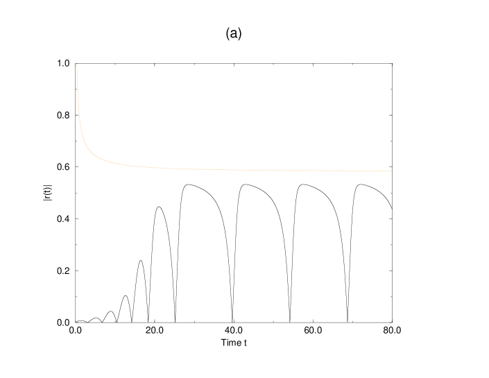
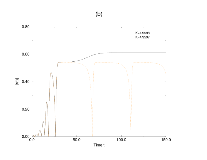
FIG. 9.: (a) Time evolution of the order parameter in the parameter region $\omega_{0}=1.5$, $D=1$ and $K=4.95$ where SW and SS solutions are both stable: different initial data evolve to one of these solutions. (b) Details on the end of the SW solution branch and abrupt transition to the SS at $K=4.9598$.

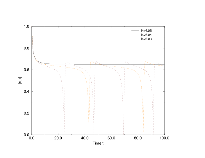
FIG. 10.: Time evolution of the order parameter in the parameter region $\omega_{0}=2$, $D=1$ for $K=6.03,6.04,6.05$ illustrating the smooth transition between the stable SW and upper SS solution branches. For this value of $\omega_{0}$ there is no bistability between SW and SS solutions.

REFERENCES

• [1] E-address bonilla@ing.uc3m.es. Author to whom all correspondence should be addressed.
• [2] E-address conrad@ulyses.ffn.ub.es
• [3] E-address spigler@ulam.dmsa.unipd.it
• [4] K.Y. Tsang, S.H. Strogatz, and K. Wiesenfeld, Reversibility and noise sensitivity of Josephson arrays, Phys. Rev. Lett. 66, (1991), 1094-1097.
• [5] K.Y. Tsang, R.E. Mirollo, S.H. Strogatz, and K. Wiesenfeld, Dynamics of a globally coupled oscillator array, Physica D 48, (1991), 102-112.
• [6] S.H. Strogatz, C.M. Marcus, R.M. Westervelt and R.E. Mirollo, Simple model of collective transport with phase slippage. Phys. Rev. Lett. 61, (1988) 2380-2383.
• [7] A.T. Winfree, Biological rhythms and the behavior of populations of coupled oscillators, J. Theoret. Biol. 16, (1967), 15-42.
• [8] S. H. Strogatz, Norbert Wiener’s brain waves, edited by S. Levin. Lect. N. Biomath. 100, Springer, N. Y. 1994.
• [9] R. E. Mirollo and S. H. Strogatz, Synchronization of the pulse-coupled biological oscillators, SIAM J. Appl. Math. 50, (1990), 1645-1662.
• [10] C.M. Gray and W. Singer, Stimulus specific neuronal oscillations in the cat visual cortex: a cortical functional unit, Soc. Neurosci. Abst. 13, (1987) 13.
• [11] Y. Kuramoto, Chemical Oscillations, Waves and Turbulence. Springer, N. Y. 1984.
• [12] D. G. Aronson, G. B. Ermentrout and N. J. Kopell, Amplitude response of coupled oscillators, Physica D 41, (1990) 403-449.
• [13] Y. Kuramoto, Self-entrainment of a population of coupled nonlinear oscillators; in International Symposium on Mathematical Problems in Theoretical Physics, H. Araki ed., Lecture Notes in Physics 39, Springer, N. Y. 1975. pp. 420-422.
• [14] H. Sakaguchi, Cooperative phenomena in coupled oscillator systems under external fields. Prog. Theor. Phys. 79, (1988) 39-46.
• [15] S. H. Strogatz and R. E. Mirollo, Phase-locking and critical phenomena in lattices of coupled nonlinear oscillators with random intrinsic frequencies. Physica D 31, (1988) 143-168.
• [16] E. D. Lumer and B. A. Huberman, Hierarchical dynamics in large assemblies of interacting oscillators. Phys. Lett. A 160, (1991) 227-230.
• [17] L. L. Bonilla and J. M. Casado, Dynamics of a soft-spin van Hemmen model. I. Phase and bifurcation diagrams for stationary distributions. J. Statist. Phys. 56, (1989) 113-125.
• [18] C. J. Pérez Vicente, A. Arenas and L. L. Bonilla, On the short time dynamics of networks of Hebbian coupled oscillators. J. Phys. A 29, (1996) L9-L16.
• [19] L.L. Bonilla, C.J. Pérez Vicente and J.M. Rubí, Glassy synchronization in a population of coupled oscillators. J. Stat. Phys. 70, (1993) 921-937.
• [20] H. Sompolinsky, D. Golomb and D. Kleinfeld, Cooperative dynamics in visual processing. Phys. Rev. A 43, (1991) 6990-7011.
• [21] L. L. Bonilla, Stable Probability Densities and Phase Transitions for Mean-Field Models in the Thermodynamic Limit, J. Statist. Phys. 46, (1987) 659-678.
• [22] S.H. Strogatz and R.E. Mirollo, Stability of incoherence in a population of coupled oscillators, J. Statist. Phys. 63, (1991), 613-635.
• [23] L. L. Bonilla, J. C. Neu, and R. Spigler, Nonlinear stability of incoherence and collective synchronization in a population of coupled oscillators, J. Statist. Phys. 67, (1992), 313-330.
• [24] J.D. Crawford, Amplitude expansion for instabilities in populations of globally-coupled oscillators, J. Statist. Phys. 74, (1994), 1047-1084.
• [25] K. Okuda and Y. Kuramoto, Mutual entrainment between populations of coupled oscillators, Prog. Theor. Phys. 86, (1991), 1159-1176.
• [26] G. Dangelmayr and E. Knobloch, The Takens-Bogdanov bifurcation with the O(2)-symmetry, Phil. Trans. R. Soc. Lond. A 322, (1987), 243-279.
• [27] J. Lin and P. B. Kahn, Averaging methods in the delayed logistic equation. J. Math. Biol. 10 (1980), 89-96. J. Lin and P. B. Kahn, Phase and amplitude instability in delay-diffusion population models. J. Math. Biol. 13 (1982), 383-393.
• [28] J. D. Cole and J. Kevorkian, Multiple Scale and Singular Perturbation Methods, Springer, New York, 1996.
Refer to caption