Asymptotic description of transients and synchronized states of globally coupled oscillators

Abstract

A two-time scale asymptotic method has been introduced to analyze the multimodal mean-field Kuramoto-Sakaguchi model of oscillator synchronization in the high-frequency limit. The method allows to uncouple the probability density in different components corresponding to the different peaks of the oscillator frequency distribution. Each component evolves toward a stationary state in a comoving frame and the overall order parameter can be reconstructed by combining them. Synchronized phases are a combination of traveling waves and incoherent solutions depending on parameter values. Our results agree very well with direct numerical simulations of the nonlinear Fokker-Planck equation for the probability density. Numerical results have been obtained by finite differences and a spectral method in the particular case of bimodal (symmetric and asymmetric) frequency distribution with or without external field. We also recover in a very easy and intuitive way the only other known analytical results: those corresponding to reflection-symmetric bimodal frequency distributions near bifurcation points.

I Introduction

In recent years mathematical modeling and analysis of synchronization phenomena received increased attention because of its occurrence in quite different fields, such as solid state physics [3, 4, 5], biological systems [6, 7, 8, 9], chemical reactions [10], etc. These phenomena can be modeled in terms of populations of interacting, nonlinearly coupled oscillators as first proposed by Winfree [6]. While the dynamic behavior of a small number of oscillators can be quite interesting [11], here we are concerned with synchronization as a collective phenomenon for large populations of interacting oscillators [7]. Then we can describe populations of oscillators interacting via simple couplings (e.g., all-to-all, mean-field couplings) by means of kinetic equations for one-oscillator densities [12, 7, 13]. Many recent studies of synchronization phenomena combine numerical simulations with linear stability and bifurcation analyses of particular (stable) incoherent and synchronized states [13, 14, 15, 16]. These works have described the onset of synchronized phases and, near degenerate bifurcation points, synchronized phases from their beginning to their end in the corresponding bifurcation diagram [17]. In this paper we introduce a high-frequency singular perturbation method which describes (in a conveniently analytical manner) synchronized phases far from bifurcation points. The method nicely agrees with the results of numerical simulations.

These ideas may be made concrete in a simple model put forth by Kuramoto and Sakaguchi [18, 19] (see also [7]). It consists of a population of coupled phase oscillators, $\theta_{j}(t)$, having natural frequencies $\omega_{j}$ distributed with a given probability density $g(\omega)$, and subject to the action of an external field $h_{j}$ which is distributed with a probability density $f(h)$,

$$\dot{\theta_{j}}=\omega_{j}+\xi_{j}(t)-h_{j}\,\sin\theta_{j}+\sum_{l=1}^{N}K_{jl}\sin(\theta_{l}-\theta_{j}),\quad\quad j=1,\ldots,N.$$ (1)

Here $\xi_{j}$ are independent white noise processes with expected values

$$\langle\xi_{j}(t)\rangle=0,\ \ \ \langle\xi_{j}(t)\xi_{l}(t^{\prime})\rangle=2D\delta(t-t^{\prime})\,\delta_{jl}.$$ (2)

In the absence of external field and white noise, each oscillator tries to run independently at its own frequency while the coupling tends to synchronize it to all the others. When the coupling is sufficiently weak, the oscillators run incoherently whereas beyond a certain threshold collective synchronization appears spontaneously. So far, several particular prescriptions for the matrix $K_{jl}$ have been considered. For instance, $K_{jl}=K>0$ only when $|j-l|=1$, and $K_{jl}=0$ otherwise (next-neighbor coupling) [20]; $K_{jl}=K/N>0$ (mean-field coupling) [18, 10]; hierarchical coupling [21]; random long-range coupling [22, 23, 24] or even state dependent interactions [25]. In the mean-field case, the model (1)-(2) can be written in a convenient form by defining the (complex-valued) order-parameter

$$re^{i\psi}=\frac{1}{N}\sum_{l=1}^{N}e^{i\theta_{l}}\,.$$ (3)

Here $|r(t)|$ measures the phase coherence of the oscillators, and $\psi(t)$ measures the average phase. Then eq. (1) reads

$$\dot{\theta_{j}}=\omega_{j}-h_{j}\sin\theta_{j}+Kr\sin(\psi-\theta_{j})+\xi_{j}(t),\ \ \ j=1,2,\ldots,N.$$ (4)

In the limit of infinitely many oscillators, $N\rightarrow\infty$, a nonlinear Fokker-Planck equation (NLFPE) was derived [12, 13] for the one-oscillator probability density, $\rho(\theta,t,\omega,h)$,

$$\frac{\partial\rho}{\partial t}=D\frac{\partial^{2}\rho}{\partial\theta^{2}}-\frac{\partial}{\partial\theta}(v\rho),$$ (5)

the drift-term being given by

$$v(\theta,t,\omega)=\omega-h\sin\theta+Krsin(\psi-\theta),$$ (6)

and the order-parameter amplitude by

$$re^{i\psi}=\int_{0}^{2\pi}\!\!\int_{-\infty}^{+\infty}\!\!\int_{-\infty}^{+\infty}e^{i\theta}\rho(\theta,t,\omega,h)\,g(\omega)\,f(h)\,d\theta\,d\omega\,dh.$$ (7)

The probability density is required to be $2\pi$-periodic as a function of $\theta$ and normalized according to

$$\int_{0}^{2\pi}\rho(\theta,t,\omega,h)\,d\theta=1.$$ (8)

Mean-field models such as those described above were studied, e.g., by Strogatz and Mirollo [13] in the absence of external field and for a unimodal [$g(\omega)$ is non-increasing for $\omega>0$] frequency distribution, $g(\omega)$, having reflection symmetry, $g(-\omega)=g(\omega)$. In [13], the authors showed that for $K$ smaller than a certain value $K_{c}$, the incoherent equiprobability distribution, $\rho_{0}\equiv 1/(2\pi)$, is linearly stable, and linearly unstable for $K>K_{c}$. As $D\to 0+$, the incoherence solution is still unstable for $K>K_{c}$ [$=2/\pi g(0)$ at $D=0$], but it is neutrally stable for $K<K_{c}$: the whole spectrum of the equation linearized about $\rho_{0}$ collapses to the imaginary axis. In [14], the nonlinear stability issue was addressed, and the case of a reflection-symmetric bimodal frequency distribution was considered [$g(\omega)$ is even and it has maxima at $\omega=\pm\omega_{0}$]. In this case, new bifurcations appear, and bifurcating synchronized states have been asymptotically constructed in the neighborhood of the bifurcation values of the coupling strength. The nonlinear stability properties of such solutions were also studied for the explicit discrete example $g(\omega)={1\over 2}[\delta(\omega-\omega_{0})+\delta(\omega+\omega_{0})]$, cf. [14]. A complete bifurcation study taking into account the reflection symmetry of $g(\omega)$ was carried out by Crawford, [15]. Similar results were obtained by Okuda and Kuramoto in the related case of mutual entrainment between populations of coupled oscillators with different frequencies [16]. Furthermore, a two-parameter bifurcation analysis near the tricritical point (at which bifurcating stationary and oscillatory solution branches coalesce) allows us to visualize a global bifurcation diagram in which oscillatory solution branches may be calculated analytically from their onset to their end [17]. The effect of an external field on Kuramoto models has been analyzed in Refs. [26, 27].

In this paper we shall illustrate our high-frequency perturbation method by applying it to the generalized mean-field Kuramoto model (5)-(8). We shall assume that the frequency distribution is multimodal in the high-frequency limit: $g(\omega)$ has $m$ maxima located at $\omega_{0}\Omega_{l}$, $l=1,\ldots,m$, where $\omega_{0}\rightarrow\infty$. Then $g(\omega)\,d\omega$ tends to the limit distribution

$$\Gamma(\Omega)\,d\Omega\equiv\sum_{l=1}^{m}\alpha_{l}\,\delta(\Omega-\Omega_{l})\,d\Omega,$$ (9)

$$\mbox{with}\quad\quad\sum_{l=1}^{m}\alpha_{l}=1,\quad\mbox{and}\quad\Omega=\frac{\omega}{\omega_{0}}\,,$$ (10)

independently of the shape of $g(\omega)$ as $\omega_{0}\to\infty$. Then $g(\omega)\,d\omega$ and $\Gamma(\Omega)\,d\Omega$ may be used interchangeably when calculating any moment of the probability density [including of course the all-important order parameter (7)]. Thus any frequency distribution is equivalent to a discrete multimodal distribution in the high-frequency limit. The discrete symmetric bimodal distribution considered in [14, 17] corresponds to $m=2$, $\Omega_{l}=(-1)^{l}$, $\alpha_{l}={1\over 2}$, $l=1,2$. We shall show that the oscillator probability density splits into $m$ components, each contributing a wave rotating with frequency $\Omega_{l}\omega_{0}$ to the order parameter. The envelope of each component evolves to a stationary state as the time elapses. Thus our method yields analytical expressions for the probability density and the order parameter during the transients toward synchronized (or incoherent) phases, which agree with direct numerical simulations of the NLFPE. Since it is not a small-amplitude expansion, our method is valid well inside the regions of stable synchronized phases in the phase diagram, far from bifurcation points. Of course we have derived the method in the limit $\omega_{0}\to\infty$, but comparison with numerical simulations shows that $\omega_{0}=7$ is already close to infinity for all practical purposes.

Our numerical calculations have been carried out by means of finite difference schemes and by using a spectral method which generates a hierarchy of ordinary differential equations for moments of the probability density which include the order parameter. This method is equivalent to an expansion of the probability density in a Fourier series and it could in principle be used to reconstruct it. The moment hierarchy was derived directly from Eqs. (1)-(2) by Pérez Vicente and Ritort [28]. They assumed that arithmetic means converged to ensemble averages in the limit $N\to\infty$ [keeping $t=O(1)$], which was justified in [12]. From the moment hierarchy, Pérez Vicente and Ritort [28] also derived a nonlinear kinetic equation for a moment-generating function $\Upsilon(\theta,y,t)=\int e^{\omega y}\,\rho(\theta,t;\omega)\,g(\omega)d\omega$, which is related to functional-equation formulations of Equilibrium Statistical Mechanics [29] and fluid turbulence [30, 31].

The rest of the paper consists of a description of our method of multiple scales in Section II, comparison with numerical results in Section III, and our conclusions in Section IV.

II Method of multiple scales

The high frequency limit of the NLFPE can be analyzed by means of a method of multiple scales. Let us change variables to a comoving frame and therefore rewrite the equation as

$$\frac{\partial\rho}{\partial t} = \frac{\partial^{2}\rho}{\partial\beta^{2}}-\frac{\partial U\,\rho}{\partial\beta}\,,$$ (11)

$$U = Kr\sin(\psi-\beta-\omega t)-h\sin(\beta+\omega t)$$ (12)

$$= Kr\sin\left(\psi-\beta-{\Omega\over\varepsilon}t\right)-h\sin\left(\beta+{\Omega\over\varepsilon}t\right)\,,$$ (13)

$$\beta = \theta-\omega t\equiv\theta-{\Omega\over\varepsilon}t,$$ (14)

$$\varepsilon = \frac{1}{\omega_{0}}\ll 1.$$ (15)

The order parameter is now

$$re^{i\psi}=\sum_{j=1}^{m}\alpha_{j}e^{i\Omega_{j}{t\over\varepsilon}}\int e^{i\beta}\,\rho(\beta,t;\Omega_{j},h;\varepsilon)\,f(h)\,d\beta\,dh,$$ (16)

where we have used (9) and have implicitly assumed that h=O(1). The discrete character of the frequency distribution in the high-frequency limit makes it possible to simplify (11). In fact, Eq. (16) shows that $\rho$ may be split in different components $\rho_{j}=\rho(\beta,t;\Omega_{j},h;\varepsilon)$. Therefore we can write (11) as a coupled system of equations for the density components $\rho_{j}$:

$$\frac{\partial\rho_{j}}{\partial t} = \frac{\partial^{2}\rho_{j}}{\partial\beta^{2}}-\frac{\partial(U_{j}\,\rho_{j})}{\partial\beta}\,,$$ (17)

$$U_{j} = \mbox{Im}\left\{K\,\sum_{l=1}^{m}\alpha_{l}e^{i(\Omega_{l}-\Omega_{j})\,{t\over\varepsilon}}\int e^{i(\beta^{\prime}-\beta)}\,\rho(\beta,t;\Omega_{l},h;\varepsilon)\,f(h)\,d\beta^{\prime}dh-h\,e^{i(\beta+\Omega_{j}{t\over\varepsilon})}\right\}\,,$$ (19)

$$\int_{0}^{2\pi}\rho_{j}(\beta,t;h;\varepsilon)\,d\beta=1.$$

Eqs. (17) and (19) contain terms with rapidly-varying coefficients. It is then to be expected that an appropriate asymptotic method will be able to average them out thereby capturing the slow evolution of $\rho_{j}$ (or perhaps its envelope). This may be achieved by introducing fast and slow time scales as follows:

$$\tau=\frac{t}{\varepsilon},\quad\quad t=t.$$ (20)

We look for a distribution function which is a 2$\pi$-periodic function of $\beta$ according to the Ansatz:

$$\rho(\beta,t;\Omega,h;\varepsilon)=\rho^{(0)}(\beta,\tau,t;\Omega,h)+\varepsilon\rho^{(1)}(\beta,\tau,t;\Omega,h)+O(\varepsilon^{2}),$$ (21)

Inserting (21) into (17)-(19), we obtain the following hierarchy of equations

$${\partial\rho_{j}^{(0)}\over\partial\tau} = 0,$$ (22)

$${\partial\rho_{j}^{(1)}\over\partial\tau} = -\frac{\partial}{\partial\beta}\left\{\rho_{j}^{(0)}\,\mbox{Im}\,\left(K\sum_{l\neq j}\alpha_{j}\,e^{i(\Omega_{l}-\Omega_{j})\tau}\,e^{-i\beta}Z_{l}^{(0)})-h\,e^{i(\beta+\Omega_{j}\tau)})\right)\right\}$$ (23)

$$- {\partial\rho_{j}^{(0)}\over\partial t}+D{\partial^{2}\rho_{j}^{(0)}\over\partial\beta^{2}}-K\alpha_{j}\,\frac{\partial}{\partial\beta}\left\{\rho_{j}^{(0)}\,\mbox{Im}\,(e^{-i\beta}Z_{j}^{(0)})\right\}\,,$$ (24)

where

$$Z_{j}^{(0)}(t)=\int e^{i\eta}\rho_{j}^{(0)}(\eta,t,h)\,f(h)\,d\eta\,dh.$$ (25)

Eq. (22) implies that $\rho_{j}^{(0)}$ is independent of $\tau$. Then the terms in the right side of (24) which do not have $\tau$-dependent coefficients give rise to secular terms (unbounded on the $\tau$-time scale). The condition that no secular terms should appear is

$${\partial\rho_{j}^{(0)}\over\partial t}-D{\partial^{2}\rho_{j}^{(0)}\over\partial\beta^{2}}+K\alpha_{j}\,\frac{\partial}{\partial\beta}\left\{\rho_{j}^{(0)}\,\mbox{Im}\,(e^{-i\beta}Z_{j}^{(0)})\right\}=0.$$ (26)

This equation should be solved for $\rho_{j}^{(0)}$ together with (25), the normalization condition

$$\int_{0}^{2\pi}\rho_{j}^{(0)}(\beta,t;h)\,d\beta=1,$$ (27)

and an appropriate initial condition. We see that, except for the $h$-integration in (25), this problem is equivalent to solving a NLFPE with frequency distribution $g(\omega)=\delta(\omega)$, (identical oscillators) and coupling constant $K_{j}=K\alpha_{j}$. If the initial condition is independent of the external field $h$, we know that the solution of the previous NLFPE evolves towards a stationary state as time elapses [13]. If the initial condition depends on $h$, all we can say is that $\int\rho_{j}^{(0)}(\beta,t;h)\,f(h)\,dh$ tends to a stationary state independent of $h$ as $t\to\infty$. In both cases all possible stationary states are solutions of Eqs. (28)-(29) below [14]

$$\rho_{j}^{(0)}(\beta)=\frac{e^{K\alpha_{j}R_{j}D^{-1}\cos(\Psi_{j}-\beta)}\,\int_{0}^{2\pi}d\beta^{\prime}\,e^{-K\alpha_{j}R_{j}D^{-1}\cos(\Psi_{j}-\beta-\beta^{\prime})}}{\int_{0}^{2\pi}d\beta\,e^{K\alpha_{j}R_{j}D^{-1}\cos(\Psi_{j}-\beta)}\,\int_{0}^{2\pi}d\beta^{\prime}\,e^{-K\alpha_{j}R_{j}D^{-1}\cos(\Psi_{j}-\beta-\beta^{\prime})}}\,.$$ (28)

The order parameter $R_{j}e^{i\Psi_{j}}$ is calculated by inserting (28) into (25):

$$R_{j}e^{i\Psi_{j}}=\int_{0}^{2\pi}e^{i\eta}\rho_{j}^{(0)}(\eta)\,d\eta\equiv\lim_{t\to\infty}Z_{j}^{(0)}(t).$$ (29)

For $K\alpha_{j}<2D$, the only stationary solution is $\rho_{j}^{(0)}={1\over 2\pi}$ (incoherence), which is stable. At $K\alpha_{j}=2D$, a stable branch of synchronized solutions bifurcates supercritically from incoherence. They exist for all $K\alpha_{j}>2D$.

The overall order parameter (16) is given by

$$re^{i\psi}=\sum_{j=1}^{m}\alpha_{j}\,R_{j}\,e^{i(\Omega_{j}\tau+\Psi_{j})}+O(\varepsilon)\,.$$ (30)

To find $\psi$, we multiply both sides of (30) by $e^{-i\psi}$, and then take imaginary and real parts. After a little algebra, we obtain

$$\tan\psi=\frac{\sum_{j=1}^{m}\alpha_{j}\,R_{j}\,\sin(\Omega_{j}\tau+\Psi_{j})}{\sum_{j=1}^{m}\alpha_{j}\,R_{j}\,\cos(\Omega_{j}\tau+\Psi_{j})}\,,$$ (31)

$$r=\sum_{j=1}^{m}\alpha_{j}\,R_{j}\,\cos(\Omega_{j}\tau+\Psi_{j}-\psi)\,.$$ (32)

Notice that $r$ in (32) may be negative, positive or zero. Then the amplitude of the overall order parameter is $|r(t)|$.

Let us now consider, for the sake of definiteness, the special case of an asymmetric bimodal frequency distribution, with zero external field,

$$\Gamma(\omega)=\alpha\,\delta(\Omega-1)+(1-\alpha)\,\delta(\Omega+1),\quad 0<\alpha<1,\quad\quad f(h)=\delta(h),$$ (33)

and analyze the possible synchronized states. Eqs. (31) and (32) become

$$\tan\psi=\frac{\alpha\,R_{+}\,\sin(\Psi_{+}+\tau)+(1-\alpha)\,R_{-}\,\sin(\Psi_{-}-\tau)}{\alpha\,R_{+}\,\cos(\Psi_{+}+\tau)+(1-\alpha)\,R_{-}\,\cos(\Psi_{-}-\tau)}\,,$$ (34)

$$r=\alpha R_{+}\cos(\Psi_{+}+\tau-\psi)+(1-\alpha)R_{-}\cos(\Psi_{-}-\tau-\psi).$$ (35)

Let us now assume that $\alpha<1/2$ to be specific. Then we have the following possibilities depending on the value of the coupling constant:

1. If $0<K<2D/(1-\alpha)$, the incoherent solution $\rho=1/(2\pi)$ is stable and it is the only possible stationary solution.

2. If $2D/(1-\alpha)<K<2D/\alpha$, a globally stable partially synchronized solution issues forth from incoherence at $K=2D/(1-\alpha)$. It has $R_{+}=0$, $\psi=\Psi_{-}-\tau$, and $r=(1-\alpha)\,R_{-}$. Its component $\rho_{+}=1/(2\pi)$ is incoherent while its component $\rho_{-}$ is synchronized according to Eq. (28). The overall effect is having a traveling wave solution (rotating clockwisely), once the angular variable $\beta$ is changed back to $\theta$ according to (14).

3. If $K>2D/\alpha$, the component $\rho_{+}$ becomes partially synchronized too. The probability density then has traveling wave components rotating clockwisely and anticlockwisely. Their order parameters have different strengths and $R_{-}>R_{+}$ if $\alpha<1/2$.

When $\alpha=1/2$, both traveling wave components appear at the same value of the coupling constant, $K=4D$, and have equal strength: $R_{+}=R_{-}\equiv R$, $\Psi_{+}=\Psi_{-}\equiv\Psi$. $R$ is the amplitude of the order parameter corresponding to a unimodal frequency distribution and a coupling constant $K_{+}=K_{-}=\alpha K=K/2$. Then (34) and (35) imply that $\psi=\Psi+q\pi$ ($q$ is an integer number) and $r=R\,\cos(\omega_{0}t+q\pi)$, respectively. Thus we have obtained an overall standing wave which is stable. Of course other possible solutions are traveling waves with $R_{+}>0$, $R_{-}=0$ and $R_{+}=0$, $R_{-}>0$, which should be unstable because incoherence is an unstable solution of (28) for the corresponding stationary component $\rho_{j}$ if $K/2>2D$. These results coincide perfectly with those obtained by means of bifurcation theory in [17] and [15] for a symmetric bimodal frequency distribution ($\alpha=1/2$). To see this, we recall that the stable (up to a constant shift in the origin of time which depends on initial conditions) standing wave probability density may be approximated near a bifurcation point $K_{c}=4D$ by the following expressions [17]:

$$\rho(\theta,t,\omega)={1\over 2\pi}\,[1+\epsilon\,\sigma_{1}+O(\epsilon^{2})],\quad\quad K=4D+\epsilon^{2}\,K_{2},$$ (36)

$$\sigma_{1}=A\,\left\{\frac{e^{i(\Omega t+\theta)}}{D+i(\Omega+\omega)}+\frac{e^{i(\Omega t-\theta)}}{D+i(\Omega-\omega)}\right\}+cc,\quad\quad\Omega=\sqrt{\omega_{0}^{2}-D^{2}},$$ (37)

$$A=\sqrt{\frac{\mbox{Re}\ \alpha}{\mbox{Re}\ (\gamma+\beta)}}\ e^{i\nu\epsilon^{2}K_{2}t},\ \ \ \nu=\mbox{Im}\ \alpha-\frac{\mbox{Im}\ (\gamma+\beta)}{\mbox{Re}\ (\gamma+\beta)}\,\mbox{Re}\ \alpha\,,$$ (38)

where $cc$ means complex conjugate of the preceding term. As $\omega_{0}\to+\infty$, the parameters $\alpha$, $\beta$, $\gamma$ of (38) become [17]

$$\alpha={1\over 4}\,,\quad\beta=0\,,\quad\gamma={1\over 2DK_{2}}\,.$$ (39)

Inserting (36) to (39) in Eq. (7) for the order parameter, we obtain that $\psi$ is constant and

$$r(t)=\sqrt{K-4D\over 2D}\,\cos\omega_{0}t+O((K-K_{c}))\,.$$ (40)

Now we can compare Eq. (40) with the result of our two-time scale method, $r=R\,\cos\omega_{0}t$. $R$ is the amplitude of the order parameter corresponding to a unimodal frequency distribution and a coupling constant $K_{+}=K_{-}=\alpha K=K/2$. Near the bifurcation point, Eq. (2.12) of Ref. [14] with $K_{c}=2D$ (corresponding to $\omega_{0}=0$) and $K_{\pm}=K/2$ yields $R\sim\sqrt{(K/2-2D)/D}$, which implies exactly the result (40). It is immediate to show that both methods also lead to the same expressions for traveling wave solutions.

III Numerical results

A Spectral numerical method

Direct numerical simulations of the nonlinear Fokker-Planck system confirms our asymptotic results. We have studied discrete bimodal frequency distributions only, and used two different numerical methods. A standard finite differences method may be used to numerically integrate (5) - (8) without stability problems up to frequencies $\omega_{0}=15$ (we set $D=1$ in all our computations). For larger frequency values, time steps below 0.008 were needed and the computing cost makes this method unpractical. As indicated in the previous Section, the drift term dominates diffusion at higher frequency and the system acquires a quasi-hyperbolic character. To simulate the NLFPE at high frequencies, we propose a simple spectral method, which we will describe in the simple case of $f(h)=\delta(h)$. The idea is to find a set of ordinary differential equations for moments of the probability density related to the order parameter $r\,e^{i\psi}$:

$$x_{\pm}^{(j)}=\int_{0}^{2\pi}\rho(\theta,t,\pm\omega_{0})\,\cos[j(\psi-\theta)]\,d\theta,$$ (41)

$$y_{\pm}^{(j)}=\int_{0}^{2\pi}\rho(\theta,t,\pm\omega_{0})\,\sin[j(\psi-\theta)]\,d\theta,$$ (42)

$$r=\alpha\,x_{+}^{(1)}+(1-\alpha)\,x_{-}^{(1)}\,.$$ (43)

An infinite hierarchy of equations for these moments may be obtained by differentiating (41) and (42) with respect to time and then using the NLFPE and integration by parts to simplify the result. We obtain

$${dx_{\pm}^{(j)}\over dt}=-j^{2}\,x_{\pm}^{(j)}\pm j\omega_{0}\,y_{\pm}^{(j)}+{Kj\over 2}\,rx_{\pm}^{(j-1)}-{Kj\over 2}\,rx_{\pm}^{(j+1)}-j\,{d\psi\over dt}\,y_{\pm}^{(j)}\,,$$ (44)

$${dy_{\pm}^{(j)}\over dt}=-j^{2}\,y_{\pm}^{(j)}\mp j\omega_{0}\,x_{\pm}^{(j)}+{Kj\over 2}\,ry_{\pm}^{(j-1)}-{Kj\over 2}\,ry_{\pm}^{(j+1)}+j\,{d\psi\over dt}\,x_{\pm}^{(j)}\,,$$ (45)

$$r\,{d\psi\over dt}=\omega_{0}\,[\alpha\,x_{+}^{(1)}-(1-\alpha)\,x_{-}^{(1)}],$$ (46)

As explained in the Introduction, an equivalent hierarchy may be derived directly from the Langevin equations (1) and (2) [28]. The numerical method consists of solving (43)-(46) for $j=1,\ldots,N$, with $x_{\pm}^{(N+1)}=y_{\pm}^{(N+1)}=0$. The number of modes, $N$, should be chosen so large that the numerical results for the order parameter do not depend on it. A practical case is presented in Fig. 1 for $\omega_{0}=15$, $K=6$ and $\alpha=0.5$ for which the method of finite differences is still practical. We see that keeping four modes ($N=4$) yields already quite good agreement. Let us now describe the results of our numerical simulations.

B Results for bimodal frequency distributions and no external field

We see in Figures 2 to 6 that our analytical (asymptotic) and numerical results agree very well except for a constant phase shift which decreases as $\omega_{0}$ increases (compare figures 2 and 3 corresponding to $\omega_{0}=15$ and 200, respectively). Results for an asymmetric bimodal frequency distribution without external field are depicted in Figs. 4 to 6. As explained in the previous Section, we obtain different synchronized phases depending on the value of the coupling constant for each component of the probability density. In Figures 4 and 5, $K>2D/\alpha>2D/(1-\alpha)$. Then each component of the probability density evolves towards a synchronized phase rotating with its own frequency, $\pm\omega_{0}$, and with a constant amplitude of the order parameter given by the stationary expression (29). The overall order parameter is given by Eqs. (34)-(35) and the difference between analytical and numerical results is a constant shift in time which diminishes as the frequency $\omega_{0}$ increases. In Fig. 6 we observe the situation for a smaller coupling constant such that only one density component is synchronized. We obtain a traveling wave whose order parameter has a constant amplitude and a phase linearly decreasing with time. What happens if the frequency distribution has reflection symmetry ($\alpha=0.5$) is obvious: both density components have equal strength and therefore the phase of the order parameter is constant and its amplitude oscillates giving rise to a standing wave. This is exactly what bifurcation theory predicts [15, 17]. We have checked the excellent agreement between our present asymptotic theory, the leading-order expression for the order parameter obtained by bifurcation theory, and direct numerical simulations. The results obtained by these three methods are indistinguishable for $K=4.005$ ($K_{c}=4$).

C Results for unimodal frequency distributions and deterministic external field

Our asymptotic method yields analytical results when external fields of magnitude small compared to $\omega_{0}$ are included. For the sake of simplicity we shall present results corresponding to unimodal frequency distributions, $g(\omega)=\delta(\omega-\omega_{0})$, and external field distributions, $f(h)=\delta(h-h_{0})$. Then the probability density has a unique component rotating at frequency $\omega_{0}$ which evolves toward the stationary distribution (28) (in the comoving frame). This prediction is qualitatively supported by the numerical simulations as depicted in Fig. 7. The numerical results show that the amplitude of the order parameter oscillates about the constant value predicted by our asymptotics. The difference is of order $\varepsilon$ and it could be accounted by the first correction to the leading-order result. Fig. 8 shows that the oscillation of the order parameter amplitude is enhanced as $h_{0}$ increases. Finally all oscillations disappear if the external field becomes of the same order as the frequency, as depicted in Fig. 9. Notice that our method supports [in the limit $\omega_{0}\to\infty$, $h=O(1)$] a conjecture by Arenas and Pérez Vicente [27]: the amplitude of the order parameter in the oscillatorily synchronized state (in the presence of an external field) is given by the same expression as in the stationary state if the exact time-dependent phase of the order parameter is inserted (instead of the stationary phase). Of course it seems that the conjecture holds for a wide variety of parameter values, some outside the range of validity of our asymptotic method [27].

IV Conclusions

The high-frequency limit of the mean-field Kuramoto-Sakaguchi model of oscillator synchronization has been studied by new multiscale and numerical spectral methods. The main result of the multitime scale method is that the probability density splits into independent components corresponding to the different peaks in the oscillator frequency distribution. Each density component evolves towards a stationary distribution in a comoving frame rotating with the frequency of the corresponding peak in the oscillator frequency distribution. The overall order parameter may be calculated by putting together the partial order parameters of different components. This gives a simple picture of overall oscillatory synchronization by studying synchronization of each density component. Our method gives the same results as bifurcation theory for those parameter values where both approximations hold. Our asymptotic method also works far from bifurcation points and it agrees well with results of numerical simulations. We have used a spectral method to numerically integrate the nonlinear Fokker-Planck system for frequency values where simple finite differences break down. This method has merit in itself and should be studied in more detail separately.

V ACKNOWLEDGMENTS

We are indebted to F. Ritort and R. Spigler for fruitful discussions. We acknowledge financial support from the the Spanish DGICYT through grant PB95-0296.

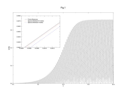
FIG. 1.: Comparison between the results of numerical simulations by finite differences and our spectral method. We have a discrete bimodal frequency distribution of the oscillators, no external field and the following parameter values: $\omega_{0}=15$, $K=6$ and $\alpha=0.5$ (frequency distribution with reflection symmetry). Differences between the methods are appreciated only on a rather fine time scale as the inset shows.

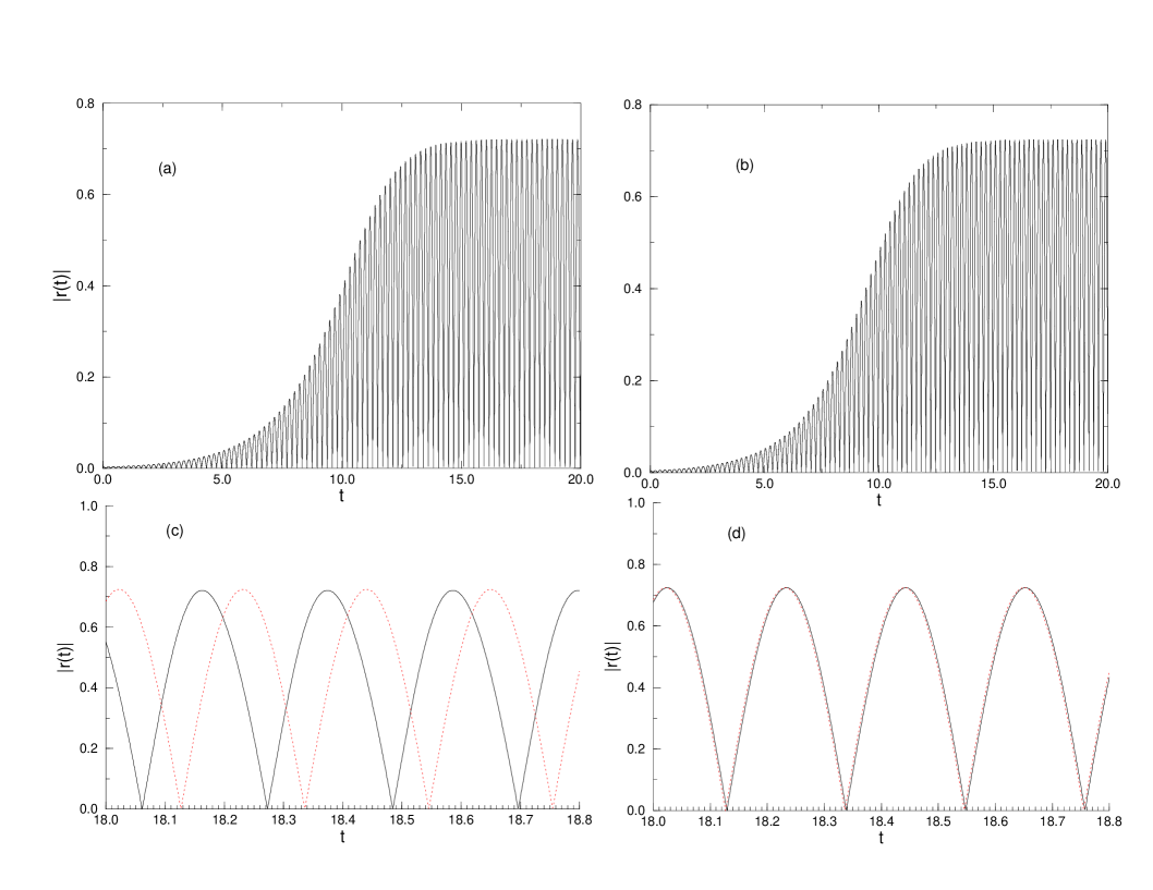
FIG. 2.: Time evolution of the order parameter amplitude $|r(t)|$ for the same parameter values of Figure 1: (a) analytical result from our leading-order asymptotics; (b) numerical simulation; (c) comparison between both results; (d) same as (c) but now we have shifted the analytical result so that $t\to t+0.055$.

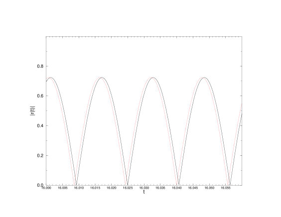
FIG. 3.: Same as Fig. 2(c) except that now $\omega_{0}=200$. Notice that the time shift between analytical and numerical results is now much smaller.

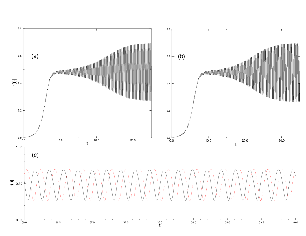
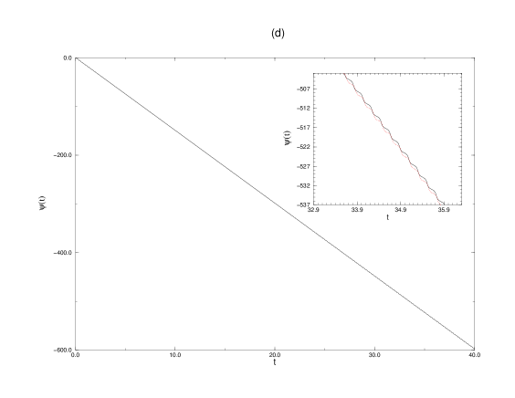
FIG. 4.: Time evolution of the order parameter $r(t)\,e^{i\psi(t)}$ for an asymmetric bimodal frequency distribution. Parameters are the same as in Fig. 1, except that now $\alpha=0.4$. (a) Analytical results for the evolution of $|r(t)|$; (b) numerical results; (c) comparison between both results; (d) evolution of the phase of the order parameter $\psi(t)$: there is only a small time shift between analytical and numerical results. Notice that for an asymmetric frequency distribution with these parameter values, $K>2/\alpha=10/3$, so that the synchronized phase is an asymmetric combination of clockwise and anticlockwise rotating traveling waves.

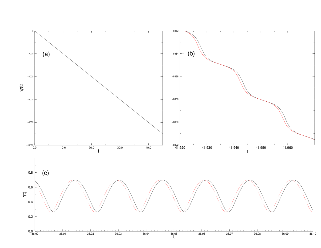
FIG. 5.: Time evolution of (a) and (b) $\psi(t)$, and (c) $|r(t)|$, for the asymmetric frequency distribution of Fig. 4 when $\omega_{0}=200$. The other parameter values are as in Fig. 4.

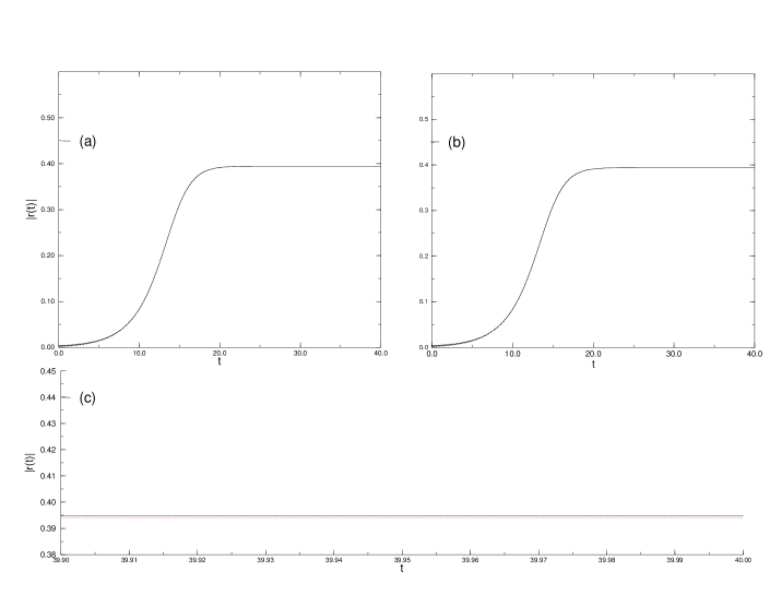
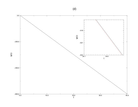
FIG. 6.: Same as Fig. 4 for a lower value of the coupling constant, $K=4.5$. Now $K\alpha=1.8<2<2.7=K(1-\alpha)$. Only the component of the probability density with negative frequency is synchronized. Then we obtain a traveling wave rotating clockwisely with constant $|r(t)|$ and phase $\psi(t)=-\omega_{0}t$.

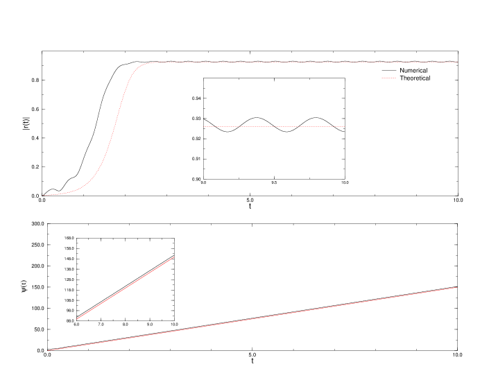
FIG. 7.: Time evolution of the amplitude and phase of the order parameter: (a) $|r(t)|$ and (b) $\psi(t)$, for the unimodal Kuramoto-Sakaguchi model. Parameter values are: $\omega_{0}=15$, $h_{0}=0.5$, and $K=7.5$. Notice the additional oscillation of the amplitude which is not predicted by our leading-order asymptotics.

FIG. 8.: Same as Fig. 7 for a larger $h_{0}$, $h_{0}=7.5$. The oscillations of the order parameter amplitude become more pronounced. Only simulation data are depicted.

FIG. 9.: Same as Fig. 7 for the following parameter values: $\omega_{0}=h_{0}=20$, and $K=6$. Notice that for such large values of the external field, a stationary state is reached for long times.

REFERENCES

- [1] E-address acebron@dulcinea.uc3m.es
- [2] E-address bonilla@ing.uc3m.es. Author to whom all correspondence should be addressed.
- [3] K.Y. Tsang, S.H. Strogatz, and K. Wiesenfeld, Reversibility and noise sensitivity of Josephson arrays, Phys. Rev. Lett. 66, (1991), 1094-1097.
- [4] K.Y. Tsang, R.E. Mirollo, S.H. Strogatz, and K. Wiesenfeld, Dynamics of a globally coupled oscillator array, Physica D 48, (1991), 102-112.
- [5] S.H. Strogatz, C.M. Marcus, R.M. Westervelt and R.E. Mirollo, Simple model of collective transport with phase slippage. Phys. Rev. Lett. 61, (1988) 2380-2383.
- [6] A.T. Winfree, Biological rhythms and the behavior of populations of coupled oscillators, J. Theoret. Biol. 16, (1967), 15-42.
- [7] S. H. Strogatz, Norbert Wiener’s brain waves, edited by S. Levin. Lect. N. Biomath. 100, Springer, N. Y. 1994.
- [8] R. E. Mirollo and S. H. Strogatz, Synchronization of the pulse-coupled biological oscillators, SIAM J. Appl. Math. 50, (1990), 1645-1662.
- [9] C.M. Gray and W. Singer, Stimulus specific neuronal oscillations in the cat visual cortex: a cortical functional unit, Soc. Neurosci. Abst. 13, (1987) 13.
- [10] Y. Kuramoto, Chemical Oscillations, Waves and Turbulence. Springer, N. Y. 1984.
- [11] D. G. Aronson, G. B. Ermentrout and N. J. Kopell, Amplitude response of coupled oscillators, Physica D 41, (1990) 403-449.
- [12] L. L. Bonilla, Stable Probability Densities and Phase Transitions for Mean-Field Models in the Thermodynamic Limit, J. Statist. Phys. 46, (1987) 659-678.
- [13] S.H. Strogatz and R.E. Mirollo, Stability of incoherence in a population of coupled oscillators, J. Statist. Phys. 63, (1991), 613-635.
- [14] L. L. Bonilla, J. C. Neu, and R. Spigler, Nonlinear stability of incoherence and collective synchronization in a population of coupled oscillators, J. Statist. Phys. 67, (1992), 313-330.
- [15] J.D. Crawford, Amplitude expansion for instabilities in populations of globally-coupled oscillators, J. Statist. Phys. 74, (1994), 1047-1084.
- [16] K. Okuda and Y. Kuramoto, Mutual entrainment between populations of coupled oscillators, Prog. Theor. Phys. 86, (1991), 1159-1176.
- [17] L. L. Bonilla, C. J. Pérez Vicente, and R. Spigler, Time-periodic phases in populations of nonlinearly coupled oscillators with bimodal frequency distributions, Physica D (1996), submitted.
- [18] Y. Kuramoto, Self-entrainment of a population of coupled nonlinear oscillators; in International Symposium on Mathematical Problems in Theoretical Physics, H. Araki ed., Lecture Notes in Physics 39, Springer, N. Y. 1975. pp. 420-422.
- [19] H. Sakaguchi, Cooperative phenomena in coupled oscillator systems under external fields. Prog. Theor. Phys. 79, (1988) 39-46.
- [20] S. H. Strogatz and R. E. Mirollo, Phase-locking and critical phenomena in lattices of coupled nonlinear oscillators with random intrinsic frequencies. Physica D 31, (1988) 143-168.
- [21] E. D. Lumer and B. A. Huberman, Hierarchical dynamics in large assemblies of interacting oscillators. Phys. Lett. A 160, (1991) 227-230.
- [22] L. L. Bonilla and J. M. Casado, Dynamics of a soft-spin van Hemmen model. I. Phase and bifurcation diagrams for stationary distributions. J. Statist. Phys. 56, (1989) 113-125.
- [23] C. J. Pérez Vicente, A. Arenas and L. L. Bonilla, On the short time dynamics of networks of Hebbian coupled oscillators. J. Phys. A 29, (1996) L9-L16.
- [24] L.L. Bonilla, C.J. Pérez Vicente and J.M. Rubí, Glassy synchronization in a population of coupled oscillators. J. Stat. Phys. 70, (1993) 921-937.
- [25] H. Sompolinsky, D. Golomb and D. Kleinfeld, Cooperative dynamics in visual processing. Phys. Rev. A 43, (1991) 6990-7011.
- [26] A. Arenas and C. J. Pérez Vicente, Phase diagram of a planar XY model with random field. Physica A 201, (1993) 614-625.
- [27] A. Arenas and C. J. Pérez Vicente, Exact long-time behavior of a network of phase oscillators under random fields. Phys. Rev. Lett. 50, (1994) 949-952.
- [28] C. J. Pérez and F. Ritort, A new approach to the dynamical solution of the Kuramoto model. Preprint, Dec. 13-1996.
- [29] R. M. Lewis and J. B. Keller, Solution of the functional equation for the statistical equilibrium of a crystal. Phys. Rev. 121, (1961) 1022-1037.
- [30] E. Hopf, Statistical hydromechanics and functional calculus. J. Rat. Mech. Anal. 1, (1952) 87-123.
- [31] R. M. Lewis and R. H. Kraichnan, A space-time functional formalism for turbulence. Comm. Pure Appl. Math. 15, (1962) 397-411.