On envelope dynamics in 2D Faraday waves

Abstract

A weakly nonlinear model for two-dimensional Faraday waves over infinite depth is derived and studied. Sideband instability of monochromatic standing waves as well as non-monochromatic solutions are studied analytically. Persistent irregular regimes are found numerically.

1 Introduction

Driven gravity-capillary waves is a well-known pattern-forming system owing its popularity to a relative simplicity and diversity of observed phenomena. Despite the wide interest in the problem, the theoretical basis of pattern formation in large-aspect-ratio systems is not yet fully understood. According to experimental data [1, 2] the complex dynamics are observed even at small supercriticalities. In the derivation of a theoretical model one must, therefore, consistently incorporate the effect of viscous dissipation, which governs the stability threshold and supercritical regimes. Furthermore, description of spatially non-homogeneous pattern formation involves “slow” space variables, whose scalings in a weakly supercritical domain depend strongly on the way how the dissipation was taken into account.

Some of earlier models [2, 3] describing the envelope dynamics of driven waves in a large-aspect-ratio system have been derived from the equations for an inviscid fluid with damping incorporated phenomenologically by adding linear damping terms to the amplitude equations. As a result, an amplitude saturation due to nonlinear damping, which remains important even for low viscosity [4], is thus overlooked. In addition, the model obtained in [3] does not possess the symmetries of the underlying physical system. The nonlinear damping terms are included in some other models [5, 6]. However, due to neglecting of the boundary layer in the derivation of [5], those terms are of higher asymptotic order than in our derivation (see below). In spite of using the consistent multiple-scales method [6] with the viscous boundary layer rigorously accounted for, due to the chosen scalings the validity of the model seems to be limited to exceedingly small supercriticalities.

In this letter we derive using results of [4] a single amplitude equation describing the evolution of one-dimensional patterns for small supercriticalities. This evolution equation is further investigated analytically and numerically.

2 Model equations

In a low-viscosity deep-water large-aspect-ratio system a packet of modes with adjacent wavenumbers becomes excited due to the parametric subharmonic resonance and locked to the (weak) forcing. In this case the principal part of a 2D motion of the free surface can be represented as a superposition of two counter-propagating small and narrow wave packets

$$\zeta(x,t)=\hat{a}e^{i\tilde{k}x+i\omega t}+\hat{b}e^{i\tilde{k}x-i\omega t}+c.c.$$ (1)

Here $\omega$ is half the driving frequency and the corresponding wavenumber $\tilde{k}$ is obtained from the dispersion relation $\omega^{2}=g\tilde{k}+(\Sigma/\rho)\tilde{k}^{3}$, where $\Sigma$ is surface tension, $g$ is the gravity acceleration and $\rho$ is the fluid density.

In the case of weak forcing and low viscosity the slow spatio-temporal evolution of the envelopes $\hat{a}(x,t),\hat{b}(x,t)$ is described by the set of equations [4]

$$\partial_{t}{\hat{a}}-s\partial_{x}{\hat{a}}=-(\gamma-\frac{1}{2}\gamma^{\frac{3}{2}})\hat{a}+if\hat{b}+(ic_{1}-p_{1}\sqrt{\gamma})|\hat{a}|^{2}\hat{a}+(ic_{2}-p_{2}\sqrt{\gamma})|\hat{b}|^{2}\hat{a},$$ (2)

$$\partial_{t}{\hat{b}}+s\partial_{x}{\hat{b}}=-(\gamma-\frac{1}{2}\gamma^{\frac{3}{2}})\hat{b}-if\hat{a}-(ic_{1}+p_{1}^{*}\sqrt{\gamma})|\hat{b}|^{2}\hat{b}-(ic_{2}+p_{2}^{*}\sqrt{\gamma})|\hat{a}|^{2}\hat{b},$$ (3)

where an asterisk denotes complex conjugate. The coefficients in eqs.(2),(3) are: a finite group speed $s=d\omega(\tilde{k})/dk$, a small linear damping $\gamma$ and the forcing amplitude $f$, and real-valued nonlinear dispersion coefficients, $c_{1},c_{2}$, given by

$$s=\sigma+\frac{1}{2},\quad\gamma=\frac{2\nu\tilde{k}^{2}}{\omega},\quad f=\frac{\hat{f}}{4}(1-\sigma),\quad\quad\sigma=\frac{\Sigma\tilde{k}^{3}}{\rho\omega^{2}},\quad c_{1}=\frac{3}{4}\sigma-\frac{3\sigma-2}{3\sigma-1},\quad c_{2}=\frac{3}{2}\sigma+\frac{6\sigma+4}{3\sigma+1}.$$

Here $\hat{f}$ is the amplitude of forcing (in units of $g$), $\sigma$ describes the nature of the wave: it is a gravity wave or a capillary wave in two limiting cases of $\sigma=0$ and $\sigma=1$, respectively.

Eqs.(2),(3) were derived in [4] from the Navier-Stokes equations using the multiple-scales method. Scalings for amplitudes and their slow variation in space and time were chosen as $\hat{a},\hat{b}\sim\gamma^{\frac{1}{2}},\partial_{x}{\hat{a}}\sim\partial_{t}{\hat{a}}\sim\gamma$. Also, following [6] a stretched coordinate was introduced to resolve the boundary layer’s dynamics. The time and space variables have been non-dimensionalized using $\omega^{-1}$ and $\tilde{k}^{-1}$, respectively, as their scales.

Higher-order corrections to the coefficients of the linear damping terms, $\gamma^{\frac{3}{2}}$ , and of the cubic terms, $p_{i}\sqrt{\gamma}$, represent, respectively, dissipation in the viscous boundary layer [8] and nonlinear interaction between potential wavefield and rotational flow in the boundary layer. Due to their cumbersome form, complex-valued coefficients $p_{i}$ are not presented here explicitly.

Imaginary parts of the coefficients of the cubic terms are responsible for saturation of the amplitude growth by tuning the wave out of the resonance (nonlinear frequency shift). Asymptotically small coefficients of the cubic terms are retained in eqs.(2),(3) since nonlinear damping can become important for small supercriticalities [4, 9], for which a simpler model is derived below.

A model similar to eqs.(2),(3) but without the higher-order damping terms was first derived using symmetry arguments and used in [2] with the coefficients estimated from the experiments. High-order nonlinear terms with real coefficients were included in [5]. However, as a result of neglecting of dissipation in the viscous boundary layer, the corresponding coefficients are asymptotically smaller ($\sim\gamma$) than in our model.

In this paper we consider the case of $p\equiv\Re(p_{1}+p_{2})>0$, in which, as we show below, subcritical solutions do not exist. We also put aside the case of second-harmonic resonance, $\sigma\approx\frac{1}{3}$, in which the coefficients $c_{1},p_{1}$ diverge indicating a breakdown of the mode.

Note, that the presence of the first spatial derivatives in eqs.(2), (3) follows only from the scaling $\partial_{x}\sim\partial_{t}\sim\gamma\sim f$ which is appropriate for the case under consideration. Indeed, according to the linear stability analysis [1, 4] the neutral curve for $f\sim\gamma\ll 1$ is defined by the equation $s^{2}(1-k)^{2}+f_{c}^{2}=f^{2}$. Above the threshold $f_{c}=\gamma-\frac{1}{2}\gamma^{\frac{3}{2}}$ the bandwidth of unstable modes grows proportionally to $f$ for a wide range of supercriticalities $\delta^{2}=(f-f_{c})/f_{c}$. Hence, the evolution of the envelopes takes place on the spatial scale $f^{-1}$, which makes the spatial derivatives in eqs.(2),(3) of the same asymptotic order as the other terms. A similar “non-traditionally” slow spatial variation of amplitude takes place in a parametrically driven oscillatory dissipative system [7].

We relate the damping parameter and supercriticality as $\gamma=\gamma_{1}^{2}\delta^{2},\,\gamma_{1}=\order(1)$. The expansions $\partial_{x}{}=\delta^{2}\partial_{x_{2}}{}+\delta^{3}\partial_{x_{3}}{}+\ldots,\quad\partial_{t}{}=\delta^{2}\partial_{t_{2}}{}+\delta^{3}\partial_{t_{3}}{}+\ldots,\quad\{\hat{a},\hat{b}\}=\delta^{\frac{3}{2}}\{a^{(1)},b^{(1)}\}+\delta^{\frac{5}{2}}\{a^{(2)},b^{(2)}\}+\ldots,\quad$ are then introduced into eqs.(2),(3) and a hierarchy of problems is obtained and solved at each order. At $\order(\delta^{7/2})$ we obtain

$$\partial_{t_{2}}{a^{(1)}}=\partial_{x_{2}}{a^{(1)}}=\partial_{t_{2}}{b^{(1)}}=\partial_{x_{2}}{b^{(1)}}=0,\quad a^{(1)}=ib^{(1)}.$$ (4)

At this order we find that the motion has a form of standing waves and the dynamics of their envelope evolve on the “slower” time- and space-scales $t_{3},x_{3}\ldots$.

At $\order(\delta^{\frac{9}{2}})$ we obtain using eq.(4) two equations

$$\partial_{t_{3}}{a^{(1)}}-s\partial_{x_{3}}{a^{(1)}}=-a^{(2)}+ib^{(2)}+ic|a^{(1)}|^{2}a^{(1)},$$ (5)

$$\partial_{t_{3}}{b^{(1)}}+s\partial_{x_{3}}{b^{(1)}}=-b^{(2)}-ia^{(2)}-ic|a^{(1)}|^{2}b^{(1)},$$ (6)

where $c\equiv c_{1}+c_{2}$. Adding eq.(5) and eq.(6) multiplied by $i$ and using eq.(4) we obtain $\partial_{t_{3}}{a^{(1)}}=\partial_{t_{3}}{b^{(1)}}=0$.

A solvability condition of eqs.(2),(3) at order $\delta^{\frac{11}{2}}$ yields an amplitude equation, which in terms of the unrescaled amplitude $\hat{a}$ and space and time variables $x,t$ reads

$$\partial_{t}{\hat{a}}=(f-f_{c})\hat{a}-p\sqrt{\gamma}|\hat{a}|^{2}\hat{a}+\frac{s^{2}}{2f}\partial^{2}_{x}{\hat{a}}+\frac{isc_{1}}{f}\partial_{x}{(|\hat{a}|^{2}\hat{a})}+\frac{isc_{2}}{f}|\hat{a}|^{2}\partial_{x}{\hat{a}}-\frac{c^{2}}{2f}|\hat{a}|^{4}\hat{a}.$$ (7)

This equation describes the slow evolution of the envelope of 2D small-amplitude driven standing waves on the surface of a weakly-viscous fluid. In what follows we consider eq.(7) with periodic boundary conditions in $0\leq x\leq L$. It turns out, that eq.(7) is also relevant for a large spectrum of $\delta/f$ [4]. In the limiting cases of very small and “large” supercriticalities there are two different mechanisms of amplitude saturation in eq.(7). For supercriticalities $(f-f_{c})/f_{c}\ll f_{c}$ the viscous cubic term is dominant and the dynamics has the relaxational form described by the Ginzburg-Landau equation [9]. In the opposite case of “large” supercriticality (or, equivalently, small damping) $\gamma\ll(f-f_{c})/f_{c}\ll 1$ saturation is due to nonlinear frequency shift provided by the three last terms in eq.(7).

In this last case, eq.(7) becomes non-typical, since the “viscous” cubic term becomes small and can be omitted, and after appropriate rescaling there is only one independent parameter. The reason for this strong mathematical degeneracy is that the coefficients of the cubic terms in eqs.(2),(3) become purely imaginary, which is a result of a weakly dissipative character of the system. In this case the only mechanism of amplitude saturation is the nonlinear frequency shift. Along with the linear dispersion (first derivative terms in eqs.(2),(3)), it leads to different types of bifurcation away from the trivial state to the monochromatic solution $\hat{a}=\hat{A}(t)\exp\{i(k-1)x)\}$ around the resonant wavenumber $k=1$: supercritical for $k>1$, and subcritical for $k<1$. This implies that the coefficient of the cubic term in the corresponding amplitude equation for $A$, changes its sign at $k=1$, and thus, in the vicinity of the minimum the saturation is provided by the quintic term.

According to eq.(7) the driven standing waves have an abnormally large amplitude, which in the typical case of $\gamma\sim(f-f_{c})/f_{c}\ll 1$ is proportional to the quartic root of the supercriticality. This peculiar steepness of the off-branching solution constitutes the substantial difference between patterns formation in a typical strongly-dissipative system and a parametrically forced weakly-dissipative oscillatory system. The second important difference is a non-traditionally slow spatial variation of the envelope, $\partial_{x}a\sim(f-f_{c})^{3/4}$, whereas for a dissipative system it is $\sim(f-f_{c})^{1/2}$ [9].

3 Analytical and numerical study of the model equation

We first show that in the subcritical domain the equilibrium state is absolutely stable. To prove this we multiply eq.(7) by $\hat{a}^{*}$ and integrate over $[0,L]$. Adding then the complex conjugate of the latter and integrating by parts we obtain

$$\frac{1}{2}\partial_{t}\int_{0}^{L}|\hat{a}|^{2}dx=\int_{0}^{L}\left((f-f_{c})|\hat{a}|^{2}-p\sqrt{\gamma}|\hat{a}|^{4}-\frac{1}{2f}\left|is\partial_{x}{\hat{a}}-c|\hat{a}|^{2}\hat{a}\right|^{2}\right)dx$$

that yields a decay of perturbations when $f<f_{c}$ and $p>0$.

Assuming now $p>0,f>f_{c}$ we rescale eq.(7) using new variables $\tau=tp^{2}f\gamma/2c^{2},\,\xi=xpf\sqrt{\gamma}/sc,\,a=\hat{a}|c|/\sqrt{pf\sqrt{\gamma}}.$ In a rescaled form eq.(7) reads

$$\partial_{\tau}{a}=\varepsilon a+\partial^{2}_{\xi}{a}-2|a|^{2}a+2i\beta\partial_{\xi}{(|a|^{2})}a+2i|a|^{2}\partial_{\xi}{a}-|a|^{4}a.$$ (8)

Eq.(8) contains only two parameters: the effective supercriticality $\varepsilon=[(f-f_{c})/f_{c}](2c^{2}/\gamma p^{2})$, and $\beta=c_{1}/c$, whose value depends on $\sigma$ and varies in a wide range.

We now consider the simplest non-trivial solution of the form $a(\xi,\tau)=A(\tau)\exp(iK\xi)$, describing a standing monochromatic (MC) wave with the modified wavenumber $k=1+Kpf\sqrt{\gamma}/{sc}$. In this case the time evolution of the amplitude has the gradient form

$$\partial_{\tau}{A}=-\partial_{A}{F},\quad\mbox{ where }F=\frac{1}{6}(K+A^{2})^{3}+\frac{1}{2}A^{4}-\frac{\varepsilon}{2}A^{2}.$$ (9)

Since $F$ is bounded from below for fixed $K$, any MC perturbation results either in the trivial solution $a\equiv 0$ or in one of the stationary solutions

$$a_{\pm}={\cal A}_{\pm}e^{iK\xi},\quad{\cal A}^{2}_{\pm}=-K-1\pm\sqrt{\varepsilon+2K+1}.$$ (10)

It follows from eqs.(9),(10) that the solution $a_{-}$, which exists for $K<-1$ and branches off the trivial solution subcritically, is unstable.

The bifurcation diagram of standing MC wave is shown in fig.1a for different $\varepsilon$. It is seen that for large values of $\varepsilon$, such that $\varepsilon f\ll 1$ (this condition supports the asymptotic method), a solution with an arbitrarily large amplitude is possible. If such a solution materializes as a result of the time evolution of a finite perturbation $|a|\sim 1$, then this would mean the failure of the model eq.(8). However, as our numerical study shows (see below), there is a mechanism of the amplitude saturation owing to the subcritical character of bifurcation of the large-amplitude solution $a_{+}$ for $K<-1$.

We now proceed to sideband (SB) stability analysis of the MC solution $a_{+}$. The perturbed solution is expressed as

$$a=e^{iK\xi}({\cal A}_{+}+\alpha_{1}e^{iq\xi+\lambda\tau}+\alpha_{2}e^{-iq\xi+\lambda^{*}\tau}).$$ (11)

Here $\alpha_{1},\alpha_{2}$ are complex amplitudes, $q$ is the perturbation of the wave number and $\lambda$ is the growth rate. Upon substitution of eq.(11) into eq.(8) we find

$$\lambda=-q^{2}B(B+K+1)\pm\sqrt{B^{2}(B+1+K)^{2}+q^{2}(K+B)(K+B+2\beta B)},\quad\mbox{ where }B={\cal A}^{2}.$$

The instability is long-wave and the threshold is defined by the minimal wavenumber allowed by the periodic constraint. For an infinite system $q_{min}\to 0$, and the threshold is defined by the equation $B=(B+K)(K+2\beta B)$. For positive $\beta$’s the SB-stability domain is adjacent to the saddle-node bifurcation curve $\varepsilon_{SN}=-2K-1$ (curve 1 in fig.1b), and shrinks when $\beta$ increases. For negative $\beta$’s the SB-stability domain widens and moves towards the center of the linear instability domain bounded by the neutral curve $\varepsilon=K^{2}$ (dotted curve in fig.1b).

We now show an existence of a stationary non-MC solution of the form $a=A(\xi)\exp(i\theta(\xi))$. For this we separate eq.(8) into real and imaginary parts to obtain

$$\varepsilon A+\partial^{2}_{\xi}{A}-2A^{3}-(\partial_{\xi}{\theta})^{2}A-2A^{3}\partial_{\xi}{\theta}-A^{5}=0,$$ (12)

$$2\partial_{\xi}{A}\partial_{\xi}{\theta}+A\partial^{2}_{\xi}{\theta}+2(2\beta+1)A^{2}\partial_{\xi}{A}=0.$$ (13)

Eq.(13) can be integrated allowing an elimination of the phase $\theta$ from eq.(12):

$$\partial^{2}_{\xi}{A}=-\partial_{A}{U},\quad\mbox{ where }U=\frac{C^{2}}{2A^{2}}+\frac{A^{2}}{2}(\varepsilon+2C\beta-C)-\frac{1}{2}A^{4}-\frac{A^{6}}{24}(1-2\beta)^{2}.$$ (14)

This equation describes a particle motion in a potential field, where $\xi$ is interpreted as time. The potential $U$ has a local minimum at $A={\cal A}_{1}$. A periodic motion of the particle around the minimum corresponds to a non-MC solution periodic in space. Two integration constants can be determined from the periodicity conditions for the amplitude $A$ and the local wavenumber $\partial_{\xi}\theta$. In the presence of the periodic constraint one finds a countable family of periodic solutions, which are spatially non-MC. In an unbounded system (in the absence of periodic constraint) the continuum of solutions exists, including a stationary solitary wave corresponding to a homoclinic orbit in the phase plane of eq.(14).

We have also investigated numerically Eq.(8) along with periodic boundary conditions to study more complex non-stationary regimes. We used a pseudo-spectral method with a second-order time-marching and up to $256$ spatial Fourier modes. In a full agreement with our stability analysis, the SB-unstable MC solution breaks down if it is initially perturbed by a sideband perturbation. The resulting regime depends on whether for a given $\varepsilon$, all SB-stable solutions are deeply subcritical (e.g. $\beta=2,\varepsilon=8$ in fig.1b) or there exist SB-stable solutions in a supercritical domain (e.g. $\beta=-1$ in fig.1b).

In the first case the breakdown of an unstable solution leads (via a phase-slip in the underlying standing waves) to onset of the stationary MC waves with a different wavenumber from the SB-stability domain (see fig.2a). This is a typical behavior for a negative or slightly positive $\beta$, for which the domains of SB-stability and instability of the trivial solution overlap for moderate $\varepsilon$. Non-MC solutions studied above analytically, were not detected in our numerical simulations. They seem to belong to unstable manifolds separating the basins of attraction of MC solutions.

For positive $\beta$ and large values of $\varepsilon$, for which SB-stable solutions are in the subcritical domain (see the horizontal dashed line in fig.1b), the instability of MC waves typically results in onset of an irregular regime. The time-evolution of the Fourier spectrum for $\beta=1,\delta=8$ is shown in fig.2b. This irregular behavior was checked using a refined numerical scheme during a rather long calculation ($\tau=10^{4}$), in which it remained qualitatively the same.

In our opinion this irregular behavior is a result of two factors: (i) SB instability of MC solutions with moderate $K$, and (ii) subcritical character of bifurcation of SB-stable MC solutions, which does not allow the perturbations with large negative $K$ to attain their stationary values.

To summarize our results, a new evolution equation describing the weakly supercritical regimes of driven surface waves was derived and studied. Its quintic form results in solutions of a non-traditionally large amplitude. The sideband instability of a MC wave leads to the onset of either a MC wave with a different wavenumber or an irregular motion.

We thank A.A.Nepomnyashchy for helpful discussions. This work was supported by the Center for Absorption in Science, Ministry of Immigrant Absorption, State of Israel (to I. K.), and by Y.Winograd Chair of Fluid Mechanics and Heat Transfer at Technion. A.O. was partially supported by the Fund for the Promotion of Research at the Technion.

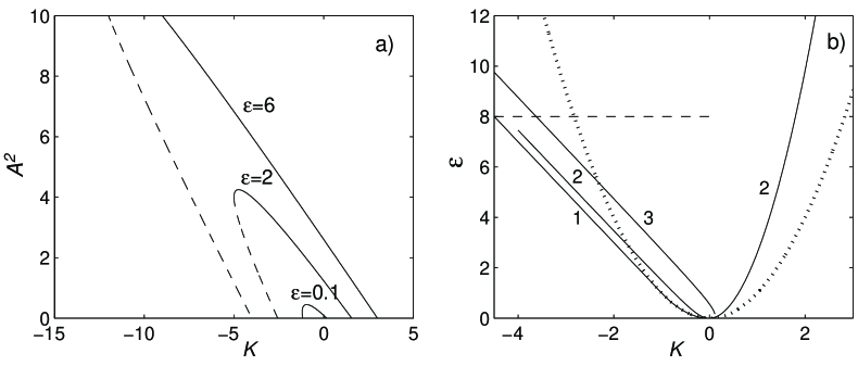
Figure 1: Bifurcation diagram (a) and stability map (b) of the MC solutions. In (a) stable and unstable branches are shown by solid and dashed curves, respectively. The dotted curve in (b) denotes the linear stability threshold of the trivial state. The domain of SB-stability of the MC solution for $\beta=-1$ is bounded from below by curve 2, whereas for $\beta=2$ it is contained between the saddle-node curve 1 and curve 3.

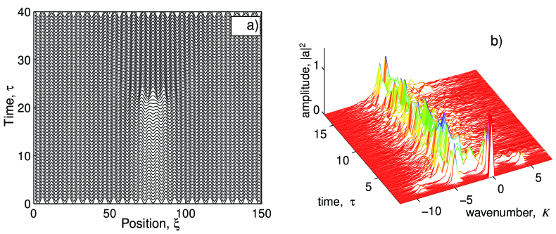
Figure 2: SB-instability of the resonant $(K=0)$ standing MC wave leading for $\beta=-1$ (a) to onset of MC wave with a different wavenumber, and for $\beta=2$ (b) to a persistent irregular pulsing (shown in Fourier space). The bandwidth of the pulsing is shown in fig.1b by the horizontal crossing line.

References

- [1] \NameChristiansen B., Alstrøm P. \AndLevinsen M.T. \ReviewJ. Fluid Mech. \Vol 291\Year1995 \Page323.
- [2] \NameEzerskii A.B., Rabinovich M.I., Reutov V.P. \AndStarobinets I.M. \Review Sov. Phys., JETP \Vol64 \Year1986 \Page1228.
- [3] \NameMiles J. \ReviewJ. Fluid Mech. \Vol148, \Year1984 \Page451.
- [4] \NameKeller I., Oron A. \AndBar-Yoseph P.Z. (in preparation).
- [5] \NameMilner S.T. \ReviewJ. Fluid Mech. \Vol225 \Year1991 \Page81.
- [6] \NameLyubimov D.V. \AndCherepanov A. A. \BookCertain problems of the Stability of a Liquid Surface, \ReviewPreprint, Ural Scientific Center, Acad. of Sci. of USSR, (Sverdlovsk) \Year1984 (in Russian).
- [7] \NameKeller I., Oron A. \AndBar-Yoseph P.Z. \ReviewPhys. Rev. E \Vol55 \Year1997 \Page3743.
- [8] Viñals J., personal communication.
- [9] \NameCross M.C. \AndHohenberg P.C. \ReviewRev. Mod. Phys. \Vol65 \Year1993 \Page851.