Unicellular algal growth: A biomechanical
approach to cell wall dynamics

Abstract

We present a model for unicellular algal growth as motivated by several experiments implicating the importance of calcium ions and “loosening” enzymes in morphogenesis. A growing cell at rest in a diffusive calcium solution is viewed as an elastic shell on short timescales. For a given turgor pressure, we calculate the stressed shapes of the wall elements whose elastic properties are determined by Young’s modulus and the thickness of the wall. The local enzyme concentration then determines the rate at which the unstressed shape of a wall element relaxes toward its stressed shape. The local wall thickness is calculated from the calcium-mediated addition of material and thinning due to elongation. We use this model to calculate growth rates for small perturbations to a circular cell. We find an instability related to modulations of the wall thickness, leading to growth rates which peak at a finite wave number.

In recent years, there has been increasing interest in models of unicellular growth. Specific examples include dendritic branching in neuronal growth [1, 2] and the broadening and branching of lobes in unicellular algal growth [3, 4, 5]. The algal models have ranged from purely geometrical models (analogous to the geometrical models of dendritic growth in solidification [6]) to one which combines the geometric formalism with a diffusive “morphogen” field. At the same time, a wealth of experimental information regarding unicellular morphogenesis has been provided by studies of the larger species of the alga Micrasterias. Morphogenesis in Micrasterias proceeds by a very well-ordered sequence of tip-splitting and lobe-broadening, culminating in elegant fan-shapes (Fig.1) which are reminiscent of the patterns seen in unstable diffusion-controlled growth[7]. This paper is devoted to the construction of a new model for this process, a model built on the dynamics of the cell wall.

Although some of the details remain elusive, a general picture of cell growth in algae has emerged from experiment. In order for the cell wall to elongate without thinning indefinitely, vesicles containing the appropriate building materials are synthesized within the cytoplasm and then travel toward the cell periphery where the fusion of vesicles with the cell membrane is thought to be mediated by calcium ions [8]. In particular, growing tips of Micrasterias exhibit high concentrations of membrane-associated calcium [8, 9], enabling them to fuse vesicles in much larger quantities than other areas of the cell wall [10]. Meanwhile, there is evidence that calcium concentration does not vary significantly within the body of the cell itself [16], perhaps implying that the relevant diffusive processes occur outside the cell body even as they modulate the concentration at the cell wall.

Experiments that halt growth by reducing turgor pressure demonstrate that elongation is (at least in part) a response to the stresses in the cell wall [10]. In addition, it has long been believed that a “loosening factor” must be present to allow the fibers making up the wall to slip past each other during elongation (e.g. the protein “expansin”[11]). Since most elongation occurs at the cell tips  [8, 12], we might surmise that high concentrations of calcium also imply high concentrations of the “loosening” factor. These observations have led us to a simple model for cell wall dynamics in algae.

Consider a cell growing in a solution of calcium ions. We treat the cell wall as an elastic shell on short time scales, whose slow plastic deformation is then catalyzed by the concentration of a “loosening” factor. We further assume that the fusion of vesicles with the cell membrane (and subsequent discharge of the vesicle contents into the cell wall) is also a long time scale process.

We begin by discretizing the stressed shape into $N$ rods with lengths $l_{i}$ and orientations $\theta_{i}$. Likewise, the unstressed shape will consist of $N$ rods with lengths $l_{i}^{\prime}$ and orientations $\theta_{i}^{\prime}$ (and our convention hereafter will be to associate all primed quantities with the unstressed shape). The stressed shape minimizes the energy

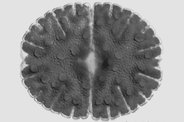
FIG. 1.: Micrasterias denticulata, diameter $\sim 200\mu m$. Picture provided by U. Meindl.

$$U=p\sum_{i=1}^{N}{l_{i}\sin{\theta_{i}}\sum_{j=1}^{i}{l_{j}\cos{\theta_{j}}}}+\sum_{i=1}^{N}{{1\over 2}\alpha_{i}\left(l_{i}-l_{i}^{\prime}\right)^{2}}+\sum_{i=1}^{N}{{1\over 2}\beta_{i}\left(\kappa_{i}-\kappa_{i}^{\prime}\right)^{2}}$$ (1)

where the angle made by the intersection of two successive rods gives rise to the curvatures $\kappa_{i}\approx\left(\theta_{i+1}-\theta_{i}\right)/\frac{1}{2}\left(l_{i+1}+l_{i}\right)$. The sums are, respectively, the energy due to the pressure ($p\oint{xdy}$, where $p<0$ for an outward pressure), the usual strain energy arising from Hooke’s Law (where $\alpha_{i}\equiv Eh_{i}/l_{i}^{\prime}$ and $E$ is Young’s modulus), and the pure bending energy of a rod (where $\beta_{i}\equiv EI_{i}l_{i}^{\prime}$ and the moment $I\equiv\int x^{2}dx$ integrated over the rod’s width for an isotropic material[13, 14]). Note that if the cell has no known rotational symmetry, we must also constrain the cell shape to be closed.

Once the stressed shape is determined, we can quasistatically calculate the calcium concentration at the cell boundary. As suggested by experiments, we assume that diffusion occurs outside the cell, with the concentration $C(R_{\infty})\equiv C_{\infty}$. We therefore solve $\nabla^{2}u=0$ in the region outside the cell, where $u\equiv(C-C_{\infty})/C_{\infty}$ is the normalized concentration and $u(R_{\infty})=0$. At the cell boundary itself, we specify the flux through the membrane with $\partial u/\partial n=j(u)/D$, where n is the outward normal to the cell surface, $j(u)$ is the inward current, and $D$ is the diffusion constant.

We then allow the unstressed shapes to relax toward the stressed configuration via

$$\frac{dl_{i}^{\prime}}{dt~{}}=\Gamma(u)\left(l_{i}-l_{i}^{\prime}\right)$$ (2)

$$\frac{d\theta_{i}^{\prime}}{dt~{}}=\Gamma(u)\left(\theta_{i}-\theta_{i}^{\prime}\right)$$ (3)

where $\Gamma(u)$ is the characteristic relaxation rate as a function of the “loosening” factor assuming, for simplicity, that it is the equivalent of the calcium concentration. Finally, if we let $\chi\left(u\right)$ be the rate at which mass (equivalently, the area $h_{i}l_{i}^{\prime}$, if the density is uniform) is added to a given rod through the fusion of vesicles, then

$$\frac{dh_{i}}{dt~{}}=\frac{\chi\left(u\right)}{l_{i}^{\prime}}-\frac{h_{i}}{l_{i}^{\prime}}\frac{dl_{i}^{\prime}}{dt~{}},$$ (4)

which completes the specification of the model.

We can now use this model to calculate the growth rates of perturbations to the cell shape. As the physics of the problem is invariant under reparametrizations, we can always choose to parametrize the unstressed membrane by dividing it into $N$ rods of equal length $l_{i}^{\prime}=a_{0}^{\prime}$. Then $\theta_{i}^{\prime}=\pi/2+\phi_{i}+b_{1}^{\prime}\delta\sin{m\phi_{i}}$ with $\phi_{i}\equiv 2\pi\left(i-1\right)/N$, specifies a perturbed circle with a curvature $\kappa^{\prime}\approx R_{0}^{\prime-1}+mb_{1}^{\prime}R_{0}^{\prime-1}\delta\cos{m\phi}$ where $R_{0}^{\prime}\equiv Na_{0}^{\prime}/2\pi$. We specify the perturbed wall thickness as $h_{i}=h_{0}+h_{1}\delta\cos{m\phi_{i}}$. We expect the stressed coordinates to have the form $l_{i}=a_{0}+a_{1}\delta\cos{m\phi_{i}}$ and $\theta_{i}=\pi/2+\phi_{i}+b_{1}\delta\sin{m\phi_{i}}$. [Note: Hereafter, we will refer to the pieces of a function $F$ expanded in $\delta$ by $F\equiv F_{0}+F_{1}\delta\cos{m\phi}$.]

In the continuum limit, we expand the total energy as $U\approx U_{0}+\delta^{2}U_{2}$, noting that the ${\cal O}(\delta)$ energy vanishes upon integration with respect to $\phi$[17]. We solve the ${\cal O}\left(\delta^{0}\right)$ problem by minimizing $U_{0}$ with respect to $a_{0}$, yielding a quartic equation for $a_{0}\equiv 2\pi R_{0}/N$.

$$R_{0}^{4}\left(p+\frac{Eh_{0}}{R_{0}^{\prime}}\right)-Eh_{0}R_{0}^{3}+EI_{0}R_{0}-EI_{0}R_{0}^{\prime}=0$$ (5)

While we could obtain the exact solution for $a_{0}$ by taking the appropriate root, it is more enlightening to expand the solution to ${\cal O}\left(p\right)$, which gives $R_{0}\approx R_{0}^{\prime}-pR_{0}^{\prime^{4}}/(Eh_{0}R_{0}^{\prime^{2}}+EI_{0})$. we can solve for the perturbations by minimizing $U_{2}$ with respect to $a_{1}$ and $b_{1}$ (a long but straightforward calculation), yielding an answer in terms of $a_{0}$ [20].

$$a_{1}=\left(a_{0}-a_{0}^{\prime}\right)\frac{pR_{0}^{8}h_{1}-\left(m^{2}-1\right)EI_{0}R_{0}R_{0}^{\prime}\left\{mI_{0}R_{0}b_{1}^{\prime}+\left[R_{0}^{3}+\frac{dI~{}}{dh_{0}}\left(R_{0}-R_{0}^{\prime}\right)\right]h_{1}\right\}}{-ph_{0}R_{0}^{8}+\left(m^{2}-1\right)EI_{0}R_{0}^{\prime}\left[h_{0}R_{0}^{4}-I_{0}\left(R_{0}-R_{0}^{\prime}\right)^{2}\right]}$$ (6)

$$b_{1}=\frac{m\left(m^{2}-1\right)EI_{0}R_{0}\left[h_{0}R_{0}^{4}-I_{0}R_{0}^{\prime}\left(R_{0}-R_{0}^{\prime}\right)\right]b_{1}^{\prime}+\left(R_{0}-R_{0}^{\prime}\right)\left\{pR_{0}^{7}-\left(m^{2}-1\right){\cal B}\right\}h_{1}}{-mph_{0}R_{0}^{8}+m\left(m^{2}-1\right)EI_{0}R_{0}^{\prime}\left[h_{0}R_{0}^{4}-I_{0}\left(R_{0}-R_{0}^{\prime}\right)^{2}\right]}$$ (7)

where ${\cal B}\equiv ER_{0}^{3}(I_{0}R_{0}^{\prime}-h_{0}\frac{dI~{}}{dh_{0}}R_{0})-EI_{0}(R_{0}-R_{0}^{\prime})(R_{0}^{3}-R_{0}^{\prime}\frac{dI~{}}{dh_{0}})$, $I_{0}\equiv I(h_{0})$, and $dI/dh_{0}$ is the derivative evaluated at $h=h_{0}$. Observe that if the bending energy is made to vanish for a cell with uniform thickness (i.e. $I_{0}=dI/dh_{0}=h_{1}=0$) we find that the stressed shape is a perfect circle ($a_{1}=b_{1}=0$). This agrees with the well-known “membrane” result that the tension $T=|p|/\kappa$, implying that curvature variations in a pliable membrane require external support[18].

We must now calculate the concentration on the stressed shape, which by direct integration of $dx_{i}=l_{i}\cos{\theta_{i}}$ and $dy_{i}=l_{i}\sin{\theta_{i}}$ is seen to have the radial perturbation $R_{1}=R_{0}\left(mb_{1}-a_{1}/a_{0}\right)/(m^{2}-1)$ for $m>1$. [21] The unperturbed solution is easily found to be $u_{0}\left(r\right)=R_{0}D^{-1}j_{0}\ln(r/R_{\infty})$ where $j_{0}=j(u_{0}(R_{0}))$. Meanwhile, the perturbed solution must have the form $u\left(r,\phi\right)\approx u_{0}\left(r\right)+cr^{-m}\delta\cos{m\phi}$. Applying the flux boundary condition, we find the concentration at the cell wall, $u(R)\equiv u_{0}+u_{1}\delta\cos{m\phi}$, to be [22]

$$u\left(R\right)\approx u_{0}\left(R_{0}\right)+\frac{j_{0}\left(m-1\right)}{mD+R_{0}\frac{\partial j}{\partial u_{0}}}R_{1}\delta\cos{m\phi},$$ (8)

where $\partial j/\partial u_{0}$ (and like expressions will) refer(s) to the derivative evaluated at $u=u_{0}(R_{0})$.

The stressed and unstressed shapes, along with the concentration just calculated, allow us to calculate $l_{i}^{\prime}\left(t+dt\right)$ and $\theta_{i}^{\prime}\left(t+dt\right)$ through equations (2) and (3). Reparameterizing the solution at $t+dt$ so that we again have equal length rods [19] yields

$$\frac{db_{1}^{\prime}}{dt~{}}=\Gamma_{0}\left(b_{1}-b_{1}^{\prime}\right)-\frac{\Gamma_{0}a_{1}}{ma_{0}^{\prime}}+\frac{\partial\Gamma~{}}{\partial u_{0}}\frac{\xi_{0}u_{1}}{m}.$$ (9)

where $\Gamma_{0}\equiv\Gamma\left(u_{0}\left(R_{0}\right)\right)$. The rate of wall-thickening can be calculated directly from (4) as

$$\frac{dh}{dt}=\frac{\chi_{0}}{a_{0}^{\prime}}-h_{0}\Gamma_{0}\xi_{0}+\left\{u_{1}\left(\frac{1}{a_{0}^{\prime}}\frac{\partial\chi~{}}{\partial u_{0}}+h_{0}\frac{\partial\Gamma~{}}{\partial u_{0}}\xi_{0}\right)+\Gamma_{0}\left(h_{1}\xi_{0}+h_{0}\frac{a_{1}}{a_{0}^{\prime}}\right)\right\}\delta\cos{m\phi}$$ (10)

where $\chi_{0}\equiv\chi\left(u_{0}\left(R_{0}\right)\right)$ and $\xi_{0}\equiv(a_{0}-a_{0}^{\prime})/a_{0}^{\prime}$. Since the average wall thickness is observed to be relatively constant during the growth of the cell[8], we must choose $\chi_{0}=a_{0}^{\prime}h_{0}\Gamma_{0}\xi_{0}$. We have tested these analytic results against simulations of the instantaneous rates and found them to be in agreement, with the error converging as $1/N^{2}.$

Though these equations are somewhat complicated, we can still use them to examine qualitative behavior in several simple situations. For definiteness, we assume that both the relaxation rate and the vesicle fusion rate increase with higher concentrations (i.e. $\partial\Gamma/\partial u_{0}$, $\partial\chi/\partial u_{0}>0$). The bending moment is taken as $I\propto h^{n}$ where $n>1$ and $h\ll R$[14]. Also, in accordance with experimental observations[8], we assume $j\left(u\right)$ causes an inward current at the cell tips (e.g. $j=u-c_{u}$ with $c_{u}$ a constant). For later reference, note that the stressed curvature is $\kappa\approx R_{0}^{-1}+R_{0}^{-1}\left(mb_{1}-a_{1}/a_{0}\right)\delta\cos{m\phi}$.

First, consider a perfectly circular cell that develops develops a slight thickening of the cell wall at $\phi=0$ (i.e. $b_{1}^{\prime}=0$ and $h_{1}>0$). For small pressures we find that (to lowest order) $b_{1}=-\xi_{0}h_{1}(I_{0}-h_{0}\frac{dI}{dh_{0}})/mI_{0}>0$ and $a_{1}=-h_{1}(a_{0}-a_{0}^{\prime})/h_{0}<0$. This implies that $\phi=0$ is a “tip” ($\kappa_{1}>0$), which is also a minimum of strain ($a_{1}<0$). This agrees with the experimental observation that wall stresses are minimized at cell tips[23]. Since $u_{1}>0$ at tips, $\Gamma_{0}h_{0}a_{1}/a_{0}$ is the only stabilizing term in (10). Therefore, if $h_{0}|a_{1}|/a_{0}$ is not too large, the thickness variations will grow, providing positive feedback to the instability which sprouted this tip.

Another interesting case is that of a perturbed cell shape which has a constant thickness (i.e. $b_{1}^{\prime}>0$ and $h_{1}=0$). To lowest order in pressure, we find that $(b_{1}-b_{1}^{\prime})\sim pb_{1}^{\prime}R_{0}^{\prime^{3}}/Eh_{0}^{n-1}\left(m^{2}-1\right)<0$, $a_{1}\sim-\left(a_{0}-a_{0}^{\prime}\right)mb_{1}^{\prime}h_{0}^{n-1}/R_{0}^{2}<0$, and $\kappa_{1}\sim mb_{1}^{\prime}$. Again, we find that the minimum strain occurs at the “tip”. Looking at equation (9), we see that $-\Gamma_{0}a_{1}/a_{0}$ is destabilizing, while $m\Gamma_{0}(b_{1}-b_{1}^{\prime})$ is stabilizing. But since $h\ll R_{0}$, we expect the net effect to stabilize $b_{1}^{\prime}$. Apparently, without modulations in the cell wall thickness, tips will be smoothed out. It is worth noting that this effect may explain the “lobe-broadening” observed in later stages of tip growth, though only full numerical simulations would demonstrate this.

A trivial yet interesting implication of equation (10) is the ability to reproduce the observed patterns of deposition of wall material when the turgor pressure is reduced [10]. Setting $p=0$ implies that $\xi_{0}=a_{1}=0$, eliminating all stabilizing influences in the thickness and implies $dh_{1}/dt=u_{1}\frac{d\chi}{du_{0}}/a_{0}^{\prime}$. That is, the thickness variations will simply follow the variations in concentration, allowing large amounts of material to collect at tips.

Finally, we can use equations (9) and (10) to obtain a pair of equations of the form $db_{1}^{\prime}/dt=c_{11}b_{1}^{\prime}+c_{12}h_{1}$ and $dh_{1}/dt=c_{21}b_{1}^{\prime}+c_{22}h_{1}$. By assuming the coefficients vary slowly and letting $b_{1}^{\prime},h_{1}\sim exp(\lambda t)$, we can obtain an expression for the quasi-static growth rates. While it is unprofitable to write the expression here, we nonetheless plot the result for a typical set of parameters in Figure 2. We find that small-scale disturbances are damped out, with the growth rate peaking at a finite wave number determined by the physical parameters of the model. In addition, we note that the $m=1$ perturbation is indeed a “zero-mode.”

FIG. 2.: Spectrum of eigenvalues in the quasistatic approximation. Growth rates ($\lambda$) are plotted against wave number ($m$) for $p=-0.001$, $E=20.0$, $h_{0}=0.4$, $R_{0}^{\prime}=10.0$, $R_{\infty}=10^{6}$, $D=1$, $j=(u+0.15)$, $\Gamma=u+0.15$, $\chi=0.12\left(u+0.15\right)$.

It is interesting to see that this relatively simple model can exhibit such rich behavior and reproduce several experimentally observed effects. This model has explicity assumed that reshaping of the cell wall is a relaxational process, wherein turgor pressure deforms the wall while enzymes allow the wall elements to slowly assume these stressed forms as their permanent forms. Our model provides a way to understand these long-standing biological assumptions analytically. It also forms the physical basis for numerical simulations that may provide further insight into the mechanisms of morphogenesis at later stages of growth.

This work has been supported in part by NSF Grant No. DMR94-15460, and by the San Diego chapter of the ARCS Foundation.

REFERENCES

• [1] Hentschel, H.G.E., Fine, A., Phys. Rev. Lett. 73, 3592-3595 (1994).
• [2] Albinet, G., Pelce, P., Europhysics Letters 33, 569-574 (1996).
• [3] Pelce, P., Sun, J., J. Theor. Biol. 160, 375-386 (1993).
• [4] Pelce, P., Pocheau, A., J. Theor. Biol. 156, 197-214 (1992).
• [5] Denet, B., Phys. Rev. E 53, 986-992 (1996).
• [6] Brower, R.C., Kessler, D.A., Koplik, J., Levine H., Phys. Rev. Lett. 51, 309-312 (1983).
• [7] D. A. Kessler, J. Koplik and H. Levine, Advances in Physics 37, 255-339 (1988).
• [8] Meindl, U.,Microbiological Reviews 57, 415-433 (1993).
• [9] Meindl, U., Lancelle, S., Hepler, P., Protoplasma 170, 104-114 (1992).
• [10] Kiermayer, O. ,Cytomorphogenesis in Plants, ed. O. Kiermayer, Springer-Verlag, Wien New York (1993), 147-189.
• [11] Cosgrove, D.,BioEssays 18, 533-540 (1996).
• [12] Nishimura, M., Ueda, K.,J. Cell Science 31, 225-231 (1978).
• [13] Landau, L.D. and Lifshitz, E.M., Theory of Elasticity, Pergamon Press , London, 1959. See pages 75-79 for a derivation of the bending energy of a rod.
• [14] For our 2d rod, $I_{i}=h_{i}^{3}/12$.
• [15] For $m>1$, $A_{1}=-\pi R_{)}^{2}\left(mb_{1}-a_{1}/a_{0}\right)^{2}/2\left(m^{2}-1\right)$ and $A_{1}=-\pi R_{0}^{2}\left(b_{1}-a_{1}/a_{0}\right)^{2}/8$ for $m=1$.
• [16] Holzinger, A.,Callaham, D., Hepler, P., Meindl, U.,European Journal of Cell Biology 67, 363-371 (1995).
• [17] The strain and bending energies are straightforward. The perturbation to the area is
$A_{1}=-\frac{1}{2}\pi R_{0}^{2}\left(mb_{1}-a_{1}/a_{0}\right)^{2}/\left(m^{2}-1\right)$ for $m>1$, and $A_{1}=-\frac{1}{8}\pi R_{0}^{2}\left(b_{1}-a_{1}/a_{0}\right)^{2}$ for $m=1$.
• [18] Calladine,C.R.,Theory of Shell Structures,Cambridge University Press, 80-86 (1983).
• [19] Given $l=A_{0}+A_{1}\delta\cos{m\phi}$ and $\theta=\pi/2+\phi+B_{1}\delta\sin{m\phi}$, the equal-length parametrization yielding the same curvature has $A_{0,new}=A_{0}$ and $B_{1,new}=B_{1}-A_{1}/mA_{0}$.
• [20] For $m=1$, the total $y$-displacement $\propto\left(b_{1}-a_{1}/a_{0}\right)$. To ensure a closed shape, we impose $b_{1}=a_{1}/a_{0}$. Minimization yields $a_{1}=-h_{1}\left(a_{0}-a_{0}^{\prime}\right)/h_{0}$, which agrees with the limit $m\rightarrow 1$ of equation (6).
• [21] For $m=1$, explicit integration of $x\left(\phi\right)$ and $y\left(\phi\right)$ shows that $R_{1}=\frac{1}{2}R_{0}\left(b_{1}+a_{1}/a_{0}\right)$.
• [22] Observe that $u_{1}=0$ for $m=1$, though technically speaking we have not required the perturbation to vanish at $r=R_{\infty}$.
• [23] Hejnowicz, Z., Heinemann, B., and Sievers, A.,Z. Pflanzenphsiol. Bd.81, 409-424 (1977).