Onset of oscillatory instabilities under stochastic modulation

Abstract

We study the effect of external stochastic modulation on a system with O(2) symmetry that exhibits a Hopf or oscillatory instability in the absence of modulation. The study includes a random component in both the control parameter of the bifurcation and in the modulation amplitude. Stability boundaries are computed by either solving the stationary Fokker-Planck equation in the vicinity of the center manifold of the underlying deterministic system whenever possible, or by direct numerical solution otherwise. If the modulation amplitude has a stochastic component, the primary bifurcation is always to standing waves at a value of the control parameter that depends on the intensity of the fluctuations. More precisely, and to contrast our results with the case of a deterministic periodic forcing, the onset of instability in the standing wave regime is shifted from its deterministic location, and the region of primary bifurcation to traveling waves disappears yielding instead standing waves at negative values of the control parameter.

I Introduction

At a Hopf bifurcation in a periodically modulated system, the trivial state loses stability to either traveling or standing waves above onset depending on the amplitude of the modulation $b$. For sufficiently small modulation amplitudes, traveling waves appear at a fixed value of the control parameter, $a_{R}$, independent of $b$. The threshold for standing waves, however, is a decreasing function of $b$. We discuss in this paper how the existence of a stochastic component in both $a_{R}$ and $b$ affects the nature of the bifurcation, as well as the stability boundaries of the trivial state. The calculations presented here are not specific to a particular system, but rather are based on the normal form equations appropriate for a Hopf bifurcation in a system with O(2) symmetry when driven by a periodic force of frequency about twice the Hopf frequency of the unperturbed system.

Detailed studies of Hopf bifurcations have been given for a large number of systems [1]. We mention, for example, the transition from straight rolls to Busse oscillations observed in Rayleigh-Bénard convection. This instability occurs in fluids of low Prandtl number ($P_{r}$) and at sufficiently large values of the Rayleigh number ($R$). For instance, it is observed in air ($P_{r}=0.71$) when $R$ reaches a value close to 6000. The instability manifests itself as a periodic transverse distortion of the rolls that propagates along their axes. Recently, Clever and co-workers [2] have studied the influence of a periodic modulation of the gravitational field on the instability. To that end, they solved numerically the time-dependent nonlinear equations for three-dimensional convection using values of $R$ above the onset of oscillatory convection. They varied the amplitude and frequency of the modulation, with the latter always set to a multiple of the fundamental (unmodulated) frequency. The main result of their study is that for moderate values of the modulation amplitude, a transition from traveling to standing waves takes place, with the system’s frequency response being either synchronous or sub-harmonic. The authors also found that, as the amplitude is further increased, this frequency locking behavior disappears and a time-dependent aperiodic regime sets in.

The onset of convection in binary fluids also occurs through an oscillatory instability when the separation ratio is negative, i.e., when the temperature field is destabilizing whereas the composition gradient is stabilizing [1]. Given the large difference in time scales between energy and mass diffusion, the process is also known as double-diffusive convection. This type of instability is commonly observed in directional solidification experiments when a crystal which is being grown upwards rejects a heavier solute. The effect of a periodic modulation of the gravitational field has been addressed theoretically by Saunders et al. [3] for a laterally unbounded fluid layer and stress free boundary conditions at the top and bottom of the layer. In the region of parameters in which the bifurcation of the unmodulated system is oscillatory, they find that below onset of the unmodulated system there exist regions of instability to stationary convection (either subharmonic or synchronous with the modulation frequency) for sufficiently large values of the modulation amplitude. For conditions above onset of the unmodulated system, the bifurcation is to traveling waves for arbitrarily small amplitudes of the modulation. These findings are in agreement with the general bifurcation diagram for a system of O(2) symmetry that will be discussed below.

Experiments on double-diffusive convection are often performed between two conducting plates which are also made permeable so as to control the solute concentration at the top and bottom of the system. As in the Rayleigh-Bénard case, the primary instability leads to a pattern of rolls, but that now propagate through the system. Experiments performed in long narrow cells of annular or rectangular geometry have shown a traveling wave pattern that is either uniform in space or confined to a small region of the cell [4] [5]. The influence of a periodic modulation of the temperature gradient has been investigated by Rehberg et al. [6] who studied convection in a water-ethanol mixture in a small rectangular cell, starting from a uniform traveling wave pattern. As was the case in the gravitationally modulated fluid layer, they observed the emergence of a standing wave structure as a periodic modulation of sufficient amplitude was added.

In the same paper, these authors report results from a much more elaborate study of the onset of electro-hydrodynamic convection in the nematic liquid crystal Merck Phase V. In this system, an electrostatic potential difference applied across the experimental cell plays a role similar to that of the temperature gradient in thermally induced convection. In order to suppress charge injection processes at the electrodes, the applied voltage is alternating at a frequency $\omega$. As its r.m.s. value is increased, the motionless state loses stability to a roll pattern, the properties of which depend on the driving frequency $\omega$. For the Merck phase V system, steady Williams rolls emerging at low frequencies give way to spatially homogeneous traveling waves as the driving frequency is increased. The authors studied the stability of these traveling waves against a small periodic modulation of the voltage. This perturbation, superimposed on top of the basic ac driving, had a small frequency $\omega_{m}$ in resonance with that of the traveling waves (i.e., $\omega_{m}\approx 2\omega_{TW}<<w$, with $\omega_{TW}$ the frequency of the traveling waves in the unmodulated state). As in the two cases described above, traveling waves were found to lose stability with respect to standing waves as the amplitude of the modulation was gradually increased. A corresponding shift in the threshold was observed, with the convecting state appearing at smaller values of the control parameter (i.e., the r.m.s voltage of the ac source).

A general description of a Hopf bifurcation in a periodically modulated system has been given by Riecke, Crawford and Knobloch [7]. Their analysis, which is briefly reviewed in Section II, involves two complex amplitude equations governing left and right traveling waves emerging at a Hopf bifurcation. The periodic modulation, which is assumed small, provides a linear coupling between the two, and leads to the excitation of standing waves under certain conditions. Different branches of the bifurcation diagram mark the onset of standing or traveling waves, and they join at a codimension-2 bifurcation point which has been observed in the electro-hydrodynamic convection experiments of Rehberg et al. The model also predicts a number of secondary instabilities which have yet to be observed experimentally.

The purpose of this paper is to extend the results summarized above to cases in which either the control parameter or the amplitude of the modulation fluctuate randomly. Although this is a quite general question, we are specially motivated by experiments conducted in a microgravity environment [8, 9]. There, the effective gravitational field is known to fluctuate in time with the amplitude of the fluctuation being two or three orders of magnitude larger than the residual steady gravitational field [10]. The frequency spectrum of the residual acceleration field, or $g$-jitter, typically comprises periodic components and a white noise background [11]. The physical origin of these disturbances lies in the many mechanical processes that take place onboard spacecraft, and their coupling to mechanical modes of the structure. A recent analysis of actual acceleration data taken during a Space Shuttle flight has shown the existence of several periodic components of frequencies in the range of a few $Hz$, and amplitudes of the order of $10^{-3}g_{E}$, where $g_{E}$ is the intensity of the Earth’s gravitational field. There appears to be also a white noise background with approximatively gaussian statistics. We attempt to present here a general framework within which to analyze the effects of such a residual field on an oscillatory instability, and therefore to provide the basis for future studies of specific systems. Two areas of concern include the appearance of undesired instabilities of some base state caused by g-jitter, and the modification in character and location of onset of a given instability because of the random component of the effective gravitational field. The specific cases of directional solidification and double diffusive convection under reduced gravity conditions have been reviewed in [12].

In the classical deterministic case, a system is said to undergo a bifurcation when its long time behavior changes qualitatively as some control parameter is continuously varied. Mathematically, this change corresponds to an exchange of stability between different solutions to the system’s governing equation(s). The nature of the bifurcation depends on that of the solutions it involves: the saddle-node, transcritical and pitchfork bifurcations, for instance, all involve two fixed-point solutions, while the Hopf bifurcation has both a fixed-point and a limit cycle. Each one of them has an associated set of equations, known as its normal form, to which any specific example transforms in a small region around its bifurcation point. The dimension of this set is equal to the smallest number of equations that can still give rise to the bifurcation (one equation in the first three examples given above, two in the Hopf case). In systems described by a larger number of equations than those involved in the normal form, the governing set of equations can be reduced close to the bifurcation point. The reduced set defines a surface in the phase space of the original equations known as the center manifold. The existence of this surface, which has the same dimension as the normal form, therefore leads to a simplified formulation of the problem, with an underlying separation of time scales in the evolution of variables on, and orthogonal to, the center manifold.

The effect of random fluctuations, both of internal and external origin, on bifurcations has been studied in considerable detail [13, 14, 15, 16]. Internal fluctuations, typically of thermal origin, enter the governing equations linearly or “additively”, scale with the inverse of the system’s size, and lead in general to so-called imperfect bifurcations: the bifurcation point is smeared into a small region of size proportional to the intensity of the fluctuations. On the contrary, externally induced fluctuations (e.g., random changes in the externally set control parameter for the bifurcation) typically enter the governing equations nonlinearly or “multiplicatively”, do not satisfy any a priori scaling with the size of the system, and the bifurcation point may remain sharp, although its position can depend on the intensity of the noise. For instance, Graham [13] has shown that a Hopf bifurcation with a fluctuating control parameter exhibits a sharp rise from the trivial state, without any shift in the location of threshold, and a small decrease in the average value of the amplitude of the new stable state compared with the deterministic case. As will be shown below for white gaussian noise, these results also hold when a periodic modulation of the control parameter is added to the system. If the intensity of this modulation is also allowed to fluctuate however, the system’s response is much more complex. It leads, among others, to shifts in threshold and to excitation of standing waves in a region of parameters in which they were previously absent.

The remainder of this paper is structured as follows: Section II briefly reviews known results on the effect of a resonant modulation on a Hopf bifurcation in a system with O(2) symmetry. The stochastic extension of the analysis is given in Sections III and IV. The former discusses the case of a stochastic component in the control parameter $a_{R}$ while the latter addresses the case of a random forcing $b$.

II Hopf bifurcation under periodic modulation

The results presented in sections III and IV extend the work of Riecke and co-workers on Hopf bifurcations in periodically driven systems [7]. For completeness, we present a brief overview of their work here. Close to a Hopf bifurcation, two complex amplitude equations are needed to describe the slow evolution of the unstable modes. Let $\Psi$ describe the state of the system. Then,

$$\Psi=u_{1}(t)e^{iqz}+u_{2}(t)e^{iqz}+\mbox{c.c.}$$ (1)

The complex amplitudes $u_{1}$ and $u_{2}$ correspond to the two eigenvalues $\pm iw_{H}$ associated with the bifurcation (with $w_{H}$ the Hopf frequency of the limit cycle), and $q$ is the characteristic wavenumber of the emerging structure (inversely proportional to the roll width in convection experiments). General equations governing the evolution of $u_{1}$ and $u_{2}$ are obtained by imposing their invariance under both spatial translations ($T:z\rightarrow z+d$) and spatial reflections ($K:z\rightarrow-z$) (O(2) symmetry). From Eq.(1), we have $T(u_{1},u_{2})=(e^{iqd}u_{1},e^{iqd}u_{2})$ and $K(u_{1},u_{2})=(u_{2}^{*},u_{1}^{*})$. Since the equations for $u_{1}$ and $u_{2}$ must remain invariant under these transformations, they have the form

$$\partial_{t}u_{1}=g_{1}u_{1}+g_{2}u_{2}$$ (2)

$$\partial_{t}u_{2}=g_{2}^{*}u_{1}+g_{1}^{*}u_{2},$$ (3)

where $g_{1}$ and $g_{2}$ are nonlinear functions of the invariants $|u_{1}|^{2}+|u_{2}|^{2}$, $u_{1}u_{2}^{*}$ and $u_{1}^{*}u_{2}$, and of the external modulation $\alpha$. The analysis is further restricted to the strong resonance case in which the frequency of the modulation is almost twice the natural frequency $w_{H}$ of the system, or $\alpha\approx be^{2iw_{H}t}$, with $b$ real. Letting $u_{1}=\eta e^{iw_{H}t}$ and $u_{2}=\zeta e^{-iw_{H}t}$ in Eq. (2) and dropping oscillatory terms, one obtains to cubic order the equations

$$\partial_{t}\eta=a\eta+b\zeta+c\eta(|\eta|^{2}+|\zeta|^{2})+g\eta|\zeta|^{2}$$ (4)

and

$$\partial_{t}\zeta=a^{*}\zeta+b\eta+c^{*}\zeta(|\eta|^{2}+|\zeta|^{2})+g^{*}\zeta|\eta|^{2},$$ (5)

governing respectively the evolution of left ($\eta$) and right ($\zeta$) traveling waves. The real part of $a$ ($a_{R}$) is the control parameter while its imaginary component ($a_{i}$) is the detuning of the wave from subharmonic resonance. The stability of the trivial state $\eta=\zeta=0$ is determined by linearizing Eqs. (4) and (5) and letting $\eta=\bar{\eta}e^{\lambda t}$ and $\zeta=\bar{\zeta}e^{\lambda t}$. Solutions of that form exist provided

$$\bar{\zeta}=\frac{b\bar{\eta}}{\lambda-a^{*}}\hskip 22.76228pt\mbox{and}\hskip 22.76228pt\lambda=a_{R}\pm\sqrt{b^{2}-a_{i}^{2}}.$$ (6)

Thus, the system undergoes either a steady bifurcation at $a_{R}=\pm\sqrt{b^{2}-a_{i}^{2}}\hskip 5.69046pt(b>a_{i})$, or a Hopf bifurcation at $a_{R}=0\hskip 5.69046pt(b<a_{i})$. The point $(a_{R},b)=(0,a_{i})$ delimiting the two corresponds to a codimension-two Takens-Bogdanov (TB) bifurcation point.

In order to study the full non-linear behavior of the system, it is useful to introduce the notation $\eta=xe^{i\varphi_{1}}$, $\zeta=ye^{i\varphi_{2}}$, $\chi=\varphi_{1}-\varphi_{2}$ and $\phi=\varphi_{1}+\varphi_{2}$. Then,

$$\partial_{t}x=a_{R}x+by\cos\chi+c_{R}x(x^{2}+y^{2})+g_{R}xy^{2}$$ (7)

$$\partial_{t}y=a_{R}y+bx\cos\chi+c_{R}y(x^{2}+y^{2})+g_{R}yx^{2}$$ (8)

$$\partial_{t}\chi=2a_{i}+n_{i}(x^{2}+y^{2})-b\sin\chi(x^{2}+y^{2})/xy,$$ (9)

with $n_{i}=2c_{i}+g_{i}$. The phase angle $\phi$ obeys the decoupled equation

$$\partial_{t}\phi=b\sin\chi(x^{2}-y^{2})/xy-g_{i}(x^{2}-y^{2}).$$ (10)

In terms of these new variables, the state of system $\Psi$ now reads

$$\Psi=x(t)e^{i[(\phi+\chi)/2+w_{H}t+qz]}+y(t)e^{i[(\phi-\chi)/2-w_{H}t+qz]}+\mbox{c.c.}$$ (11)

Equations (7),(8) and (9) admit two types of stationary solutions: standing and traveling waves. For standing waves (SW) $x=y$ and $\partial_{t}\phi=0$. In that case,

$$x^{2}=y^{2}=-M\frac{1\pm[1-N^{2}(a_{R}^{2}+a_{i}^{2}-b^{2})/M^{2}]^{1/2}}{N^{2}},$$ (12)

with $M\equiv a_{i}n_{i}+a_{R}n_{R},N^{2}\equiv n_{R}^{2}+n_{i}^{2}$ and $n_{R}\equiv 2c_{R}+g_{R}$. For traveling waves (TW), $x\neq y$ and $\partial_{t}\phi\neq 0$. They correspond to solutions

$$x^{2}_{r,l}=-a_{R}[1\pm(1-4\Delta^{2})^{1/2}]/2c_{R},\hskip 8.5359pty_{r,l}=x_{l,r},$$ (13)

with $\Delta^{2}\equiv b^{2}c_{R}^{2}/(a_{R}^{2}g_{R}^{2}+4\Omega^{2})$ and $\Omega\equiv a_{i}c_{R}-a_{r}n_{i}/2$. These solutions exist as long as $\Delta^{2}\leq 1/4$ at which point the left and right traveling waves merge to form a standing wave. The solid lines in figure 1 delimit the various regions of the stability diagram for the parameter set ($a_{i}=2,c_{R}=-1,c_{i}=2,g_{R}=-1,g_{i}=1$).

In summary, for small modulation amplitudes the system behaves exactly as in the unmodulated-modulated case: traveling waves appear at onset, which is located at $a_{R}=0$. For modulation amplitudes larger than the detuning, standing waves are excited instead, the threshold is at $a_{R}<0$, and is a decreasing function of the modulation amplitude $b$.

III Stochastic modulation of the control parameter

We begin this section with some brief considerations about the study of bifurcations in a stochastic system. As already mentioned in the introduction, we do not consider fluctuations of internal origin (thermal fluctuations, for example), but rather fluctuations in the externally set control parameters. The latter are not necessarily small, typically enter the equations nonlinearly or “multiplicatively”, and their effect is not generally a simple smearing of the deterministic threshold (the so-called imperfect bifurcation in the case of fluctuations of internal origin). Leaving aside the mathematical complexity involved in treating but the simplest cases, there remains some discussion in the multiplicative case about such basic questions as the proper definition of the threshold, or the degree of generality of the results obtained vis a vis the particular details of the model equations or the statistical properties of the fluctuating components. As there is no general agreement on these issues, we first outline our underlying assumptions here.

Our definition of instability or bifurcation point follows the work of Graham [13], and is based on the stationary solution of the Fokker-Planck equation for the system of interest. If the system bifurcates from the trivial state, the solution below threshold is a delta function centered at zero. The onset point corresponds to the value of the control parameter at which additional stationary solutions of the Fokker-Planck equation appear with some nonzero moments. Other non-normalizable stationary solutions that may appear below this onset are not considered. Second, the dimension of our starting set of equations (4) and (5) is larger than that of the unstable manifold of the deterministic case. We have adopted a center manifold reduction procedure in the stochastic case which is analogous to the one proposed by Knobloch and Wiesenfeld [17]. The stationary probability distribution function is assumed to factor into a contribution that depends only on the slow variables, and another that confines the evolution of the system to a small region around the center manifold of the underlying deterministic system. Numerical evidence is presented supporting such a factorization. We note that, unless fluctuations in the direction normal to the center manifold can be completely neglected, such a procedure is not equivalent to adiabatically eliminating the fast variables directly from the original model equations, a procedure that is standard in the study of deterministic bifurcations. The existence of a random contribution to both fast and slow time scales lies at the origin of the difference.

We now extend the model presented in section II to include a random component in $a_{R}$. Physically, this corresponds to a random component in the control parameter of the system that has a significant frequency content at $\omega\ll\omega_{H}$, and a correlation time that is small in the slow time scale emerging close to the bifurcation (inversely proportional to $a_{R}$). Under these conditions, it is also possible to assume that the random component is gaussian and white. For the three examples given in Section I, this stochastic component reflects, for example, the presence of fluctuations in either the temperature or gravitational field (Rayleigh-Bénard or double-diffusive convection) or in the applied voltage (electro-hydrodynamic convection). Results pertaining to the onset of standing waves are presented in Section III A while the transition to traveling waves is studied in Section III B. All numerical simulations reported below have been performed using an explicit integration scheme, valid to first order in $\Delta t$ (see Appendix).

A Bifurcation to standing waves

Random fluctuations in the control parameter $a_{R}$ are introduced by letting $a_{R}\rightarrow a_{R}+\xi$ (with $a_{R}$ now representing an average value). Since it is assumed gaussian and white, the noise $\xi(t)$ obeys the statistics $\langle\xi\rangle=0$ and $\langle\xi(t)\xi(t^{\prime})\rangle=2\kappa\delta(t-t^{\prime})$, with $\kappa$ its intensity. In the region corresponding to the onset of standing waves ($b>a_{i}$), it is useful to introduce the variables $A\equiv x+y$ and $Z\equiv x-y$, in terms of which Eqs. (7) to (9) become

$$\partial_{t}A=(a_{R}+b\cos\chi)A+\frac{c_{R}}{2}A(A^{2}+Z^{2})+\frac{g_{R}}{4}A(A^{2}-Z^{2})+\xi(t)A,$$ (14)

$$\partial_{t}Z=(a_{R}-b\cos\chi)Z+\frac{c_{R}}{2}Z(A^{2}+Z^{2})-\frac{g_{R}}{4}Z(A^{2}-Z^{2})+\xi(t)Z,$$ (15)

and

$$\partial_{t}\chi=2ai+\frac{n_{i}}{2}(A^{2}+Z^{2})-2b\sin\chi\frac{A^{2}+Z^{2}}{A^{2}-Z^{2}}.$$ (16)

Linear stability analysis performed in Section II showed that, in the deterministic case, standing waves appear supercritically at $a_{R}=-d\equiv-\sqrt{b^{2}-a_{i}^{2}}$. From the linear part of Eq. (14), this implies $\cos\chi=\sqrt{1-a_{i}^{2}/b^{2}}$ or $\chi=\bar{\chi}\equiv\arcsin(a_{i}/b)$ at the (deterministic) bifurcation point. The trivial solution $Z=0$ remains stable above onset as the linear coefficient $a_{R}-b\cos\chi$ in Eq. (15) is negative. Thus, an initial difference between the amplitudes of the left and right traveling waves rapidly decays to zero. This is qualitatively unchanged in the stochastic equation, as the variable $Z$ multiplies the noise $\xi(t)$ and thus suppresses the influence of fluctuations as it goes to zero. Hence, close to onset, the governing equations can be approximated by

$$\partial_{t}A=(a_{R}+b\cos\chi)A+\frac{n_{R}}{4}A^{3}+\xi(t)A,$$ (17)

and

$$\partial_{t}\chi=2ai+\frac{n_{i}}{2}A^{2}-2b\sin\chi.$$ (18)

Furthermore, in the weak noise limit, it is reasonable to expect the phase angle $\chi$ to differ only slightly from its deterministic value at onset, $\bar{\chi}$. Therefore, we introduce the variable $\theta=\chi-\bar{\chi}$ and assume $\theta<<1$. Expansion of the trigonometric functions in equations (17) and (18) yields to first order in $\theta$

$$\partial_{t}\left[\begin{array}[]{c}A\\ \theta\end{array}\right] = \left[\begin{array}[]{cc}a_{R}+d&0\\ 0&-2d\end{array}\right]\left[\begin{array}[]{c}A\\ \theta\end{array}\right]+\left[\begin{array}[]{c}\frac{n_{R}}{4}A^{3}-a_{i}\theta A\\ \frac{n_{i}}{2}A^{2}\end{array}\right]$$ (32)

$$+\left[\begin{array}[]{cc}1&0\\ 0&0\end{array}\right]\left[\begin{array}[]{c}A\\ \theta\end{array}\right]\xi(t).$$

Just above onset, the two eigenvalues $\lambda_{1}\equiv a_{R}+d$ and $\lambda_{2}\equiv-2d$ of the linearization matrix $M\equiv\left[\begin{array}[]{cc}a_{R}+d&0\\ 0&-2d\end{array}\right]$ are of opposite sign. Furthermore, $\lambda_{1}<<1$ while $|\lambda_{2}|$ is of order unity except in the close vicinity of the codimension-two bifurcation point (where $d\rightarrow 0$). This implies the existence of two different time scales in the problem, the first one of which characterizes the rapid relaxation of the system to the center manifold $\theta_{o}(A)$. To lowest order in $A$, $\theta_{o}(A)=(n_{i}/4d)A^{2}$, as seen by letting $\partial_{t}\theta=0$ in Eq. (32). The fact that $\xi(t)$ does not appear in the equation for $\theta$ allows us to neglect fluctuations away from $\theta_{o}(A)$. The subsequent evolution of the system is therefore confined to the center manifold, and we look for stationary solutions of the form ${\cal P}(A,\theta)=P(A)\delta(\theta-\theta_{o}(A))$ to the Fokker-Planck equation corresponding to Eq. (32). Explicitly, the time-independent probability distribution ${\cal P}(A,\theta)$ describing the statistical properties of the system obeys the equation

$$-\frac{\partial}{\partial A}\left\{\left[(a_{R}+d)A+\frac{n_{R}}{4}A^{3}-a_{i}\theta A+\kappa A\right]{\cal P}-\kappa\frac{\partial}{\partial A}\left[A^{2}{\cal P}\right]\right\}$$ (33)

$$-\frac{\partial}{\partial\theta}\left[\left(-2d\theta+\frac{n_{i}}{2}A^{2}+a_{i}\theta^{2}\right){\cal P}\right]=0.$$ (34)

The fast variable is eliminated from the dynamics by integrating this equation over $\theta$, with ${\cal P}(A,\theta)=P(A)\delta(\theta-\theta_{o}(A))$. The second term on the L.H.S. vanishes once the integral is performed, as it is proportional to ${\cal P}(A,\theta)$ evaluated at the limits of integration. This leaves an ordinary differential equation for $P(A)$

$$\left[(a_{R}+d)A+\left(n_{R}-\frac{a_{i}n_{i}}{d}\right)\frac{A^{3}}{4}-\kappa A\right]P-\kappa A^{2}\frac{d}{dA}P=0,$$ (35)

with solution

$$P(A)={\cal N}A^{\frac{a_{R}+d}{\kappa}-1}\exp\left[\left(n_{R}-\frac{a_{i}n_{i}}{d}\right)\frac{A^{2}}{8\kappa}\right].$$ (36)

This distribution is normalizable (with ${\cal N}=2[-(n_{R}-a_{i}n_{i}/d)/8\kappa]^{\frac{ar+d}{2\kappa}}/\Gamma[(a_{R}+d)/2\kappa]$ the normalization constant) as long as $a_{R}>-d$. Below that value, $P(A)=\delta(A)$, which implies that, just as in the deterministic case, the value $a_{R}=-d$ marks the onset of standing waves. Just above onset, the expression given in Eq. (36) exhibits a divergence at the origin (figure 2$A$). At $a_{R}=-d+\kappa$, this divergence transforms into a maximum which moves to the right as the control parameter is further increased (figure 2$B$). Both figures, corresponding to a noise intensity $\kappa=0.01$, show excellent agreement between predictions from Eq. (36) and the corresponding stationary distribution function obtained by integrating Eq. (32) numerically. The simulations were performed using a time increment $\Delta t=0.01$ and a bin size $\Delta A=0.005$. Initial conditions for $A$ and $\theta$ were chosen randomly from a uniform distribution in the interval $[0,.05]$. Results from 500 independent runs were used to compute $P(A)$. Each run consisted of five million transient iterations after which a new point was added to the statistics every 500 iterations (for a total of 1000 points per run).

From the distribution $P(A)$, the various moments of $A$ can also be determined. In particular, the standing wave’s average amplitude is given by

$$\langle A\rangle=\left[-\left(n_{R}-\frac{a_{i}n_{i}}{d}\right)\frac{1}{8\kappa}\right]^{-1/2}\frac{\Gamma\left(\frac{a_{r}+d}{2\kappa}+\frac{1}{2}\right)}{\Gamma\left(\frac{a_{r}+d}{2\kappa}\right)}.$$ (37)

As shown in figure 2$C$, results from numerical integration of both the reduced set [Eq. (32)] and the original equations for $x,y$ and $\chi$ are once again in excellent agreement with predictions from Eq. (37). As before, the values $\Delta t=0.01$ and $\kappa=0.01$ were used in each of the 50 runs performed for each value of the control parameter. Each run consisted of 11 million iterations ($10^{7}$ transient) with new points added to the statistics every 1000 time steps. At any value of the control parameter $a_{R}$, $\langle A\rangle<A_{det}$, with $A_{det}$ the amplitude of the standing wave in the deterministic case (figure 2$C$).

The statistics of the fast variable $\theta$ also follow from the analysis given above. For instance, the average phase difference between the left and right components of the standing wave is given by

$$\langle\theta\rangle = \int_{0}^{+\infty}dA\int_{-\infty}^{+\infty}d\theta\hskip 8.5359pt\theta P(A)\delta(\theta-\theta_{0}(A))=\int_{0}^{+\infty}dA\hskip 8.5359pt\theta_{0}(A)P(A)$$ (38)

$$= \frac{n_{i}}{4d}\left[\left(\frac{a_{i}n_{i}}{d}-n_{R}\right)\frac{1}{8\kappa}\right]^{-1}\frac{\Gamma\left(\frac{a_{R}+d}{2\kappa}+1\right)}{\Gamma\left(\frac{a_{R}+d}{2\kappa}\right)}=\frac{n_{i}}{d}\left[\frac{a_{i}n_{i}}{d}-n_{R}\right]^{-1}(a_{R}+d).$$ (39)

Thus the average phase difference $\langle\theta\rangle$ or, equivalently, the average second moment $\langle A^{2}\rangle$, grows linearly with the control parameter $a_{R}$. Furthermore, the slope characterizing this linear increase is independent of the noise intensity, so that both $\langle\theta\rangle$ and $\langle A^{2}\rangle$ assume their deterministic values. Figure 2$D$ compares predictions from Eq. (38) with results from numerical simulations.

The separation of time scales used to obtain Eqs. (36) and (37) gradually disappears as the codimension-two point is approached from above (i.e., as $|\lambda_{2}|=d\rightarrow 0$). Furthermore, since $\theta_{o}\propto 1/d$, fluctuations in the phase variable $\chi$ grow in the vicinity of the TB point, implying that higher order terms in $\theta$ should be kept in Eq. (32). Although the predictions from Eqs. (36) and (37) fail when $b\approx a_{i}$, numerical integration of Eqs. (7) to (9) indicates no qualitative change in the system’s behavior: the line marking the onset of standing waves from the trivial state remains un-shifted from its deterministic location, while the waves’ average amplitude above onset is comparatively smaller.

B Bifurcation to traveling waves

The transition to traveling waves can occur either from the trivial state ($b<a_{i}$) or from a pre-existing standing wave pattern ($b>a_{i}$). The TW state is characterized by a time-dependent phase angle $\phi=\varphi_{1}+\varphi_{2}$ and a finite difference in amplitude between the two wave components ($Z\neq 0$). Since $A$ and $Z$ evolve over similar time scales, the governing equations for $x,y,$ and $\chi$ can not be simplified as in Section III A. However, results from a numerical study indicate that the general conclusions of Section III A also hold in the region below the TB point. Hence, to the accuracy of the computations, no shift was detected in the location of onset. The latter was determined by computing the asymptotic amplitudes of the left and right traveling waves at different values of the control parameter $a_{R}$. For each one of these values, the complex equations (4) and (5) (with noise included in $a_{R}$) were integrated numerically two billion times, using a time step of maximum size $\Delta t=0.0005$. For all values of $b<a_{i}$ considered, the bifurcation was observed at $a_{R}=0\pm 0.002$, a value consistent with its deterministic location ($a_{R}=0$). As in Section III A, a decrease in the traveling wave’s average amplitude compared to the deterministic value was also noted above onset.

The presence of fluctuations in the control parameter affects the emergence of TW above the TB point in a different way. The transition from SW to TW, which occurs along the oblique line in figure 1, in the deterministic case, takes place over a range of control parameter values when noise is added to the system. This smearing of the bifurcation is due to the fact that both states involved in the transition have associated amplitudes $x$ and $y$ which are non-zero. Therefore, contrary to the primary bifurcation, fluctuations contribute to the dynamics on both sides of the bifurcation point. Another way to see this is to define the variable $x^{\prime}\equiv x-x_{det}$ (and, similarly, $y^{\prime}\equiv y-y_{det}$), with $x_{det}$ the deterministic value of $x$ at the bifurcation. The resulting equation for $x^{\prime}$ involves the stochastic term $(x_{det}+x^{\prime})\xi(t)$, in which the noise multiplies both the small variable $x^{\prime}$ and the constant $x_{det}$. The second component contributes additively to the dynamics, leading to an imperfect bifurcation. The transition from a standing to a traveling wave state therefore involves intermediate values of the control parameter $a_{R}$ for which the system behaves sometimes like a SW and sometimes like a TW. Numerically, this bifurcation interval was determined by monitoring the temporal evolution of the quantities $Z$ and $\partial_{t}\phi$ which are both zero if the pattern is a SW. For the parameter values given above and for all the driving intensities considered, the interval was found to include the deterministic location of onset.

IV Stochastic variation of the modulation amplitude

If the random component in the externally controlled parameters has a significant frequency content around $\omega_{H}$, the analysis given in Section III needs to be modified. We have first considered the case in which the external driving is $\alpha=\left(b+\xi(t)\right)e^{2i\omega_{H}t}$. If the correlation time of $\xi(t)$ is large compared with $1/\omega_{H}$ but short in the slow time scale emerging at the bifurcation, then $\xi(t)$ can again be assumed to be gaussian and white. A more general choice of $\alpha$ would involve both a random amplitude and phase. In that case, the coupling coefficient in the normal form is no longer real and the analysis is somewhat more involved. The resulting stability diagram is qualitatively the same than the one presented below, and will be discussed elsewhere.

A Bifurcation to standing waves

As in Section III A we first let $b=b+\xi(t)$ and rewrite Eqs. (7) to (9) in terms of the variables $A$ and $Z$. This gives

$$\partial_{t}A=(a_{R}+b\cos\chi)A+\frac{c_{R}}{2}A(A^{2}+Z^{2})+\frac{g_{R}}{4}A(A^{2}-Z^{2})+\xi(t)\cos\chi A,$$ (40)

$$\partial_{t}Z=(a_{R}-b\cos\chi)Z+\frac{c_{R}}{2}Z(A^{2}+Z^{2})-\frac{g_{R}}{4}Z(A^{2}-Z^{2})-\xi(t)\cos\chi Z$$ (41)

and

$$\partial_{t}\chi=2ai+\frac{n_{i}}{2}(A^{2}+Z^{2})-2b\sin\chi\frac{A^{2}+Z^{2}}{A^{2}-Z^{2}}-2\xi(t)\sin\chi\frac{A^{2}+Z^{2}}{A^{2}-Z^{2}}.$$ (42)

Close to onset ($a_{R}\approx-d$, with $b>a_{i}$), the variable $Z$ quickly decays to zero and consequently drops out from the above equations. Thus,

$$\partial_{t}A=(a_{R}+b\cos\chi)A+n_{R}\frac{A^{3}}{4}+\xi(t)\cos\chi A$$ (43)

and

$$\partial_{t}\chi=2a_{i}+\frac{n_{i}}{2}A^{2}-2b\sin\chi-2\xi(t)\sin\chi.$$ (44)

Due to the presence of non-linear functions of $A$ and $\chi$ in the stochastic terms, the Fokker-Planck equation corresponding to Eqs. (43) and (44) cannot be solved exactly. However, in the limit $A\rightarrow 0$, the term $n_{i}A^{2}/2$ on the R.H.S. of Eq. (44) can be neglected, effectively decoupling equation (44) from Eq. (43). Although this approximation is expected to hold only in a very small neighborhood around the bifurcation point, it is nevertheless sufficient to determine analytically the location of onset, which marks a transition from a state with $A=0$ to one in which $\langle A\rangle$ is arbitrarily small (although non-zero). The stationary probability distribution of the now independent variable $\chi$ obeys the following Fokker-Planck equation

$$\frac{dP(\chi)}{d\chi}-\left(\frac{a_{i}}{2\kappa\sin^{2}\chi}-\frac{b}{2\kappa\sin\chi}-\cot\chi\right)P(\chi)=0,$$ (45)

which yields

$$P(\chi)={\cal N}\frac{[\tan(\chi/2)]^{-b/2\kappa}}{\sin\chi}\exp\left(\frac{-a_{i}}{2\kappa\tan\chi}\right).$$ (46)

This expression for $P(\chi)$ is plotted in figure 3 for the average modulation amplitude $b=2.25$. The distribution has a maximum close to $\bar{\chi}=\arcsin(a_{i}/b)$, a divergence at $\chi=\pi$ and a minimum at some intermediate value $\chi_{m}$ (figure 3, inset). Except when $b\approx a_{i}$, $P(\chi_{m})<<1$ so that trajectories are most of the time confined to the interval $[0,\chi_{m}]$. Since the phase angle $\chi$ evolves independently of $A$ and over a much shorter time scale, it effectively acts in Eq. (43) as a second noise source, with non-zero correlation time and non-gaussian statistics. Rewriting the remaining equation for $A$ using the variables (with zero mean) $\xi^{\prime}\equiv\cos\chi-\langle\cos\chi\rangle$ and $\xi^{\prime\prime}\equiv\xi\cos\chi-\langle\xi\cos\chi\rangle$, we have

$$\partial_{t}A=(a_{R}+b\langle\cos\chi\rangle+\langle\xi(t)\cos\chi\rangle)A+n_{R}\frac{A^{3}}{4}+b\xi^{\prime}A+\xi^{\prime\prime}A,$$ (47)

which describes a pitchfork bifurcation taking place at

$$[a_{R}]_{thr}=-b\langle\cos\chi\rangle-\langle\xi\cos\chi\rangle.$$ (48)

Using the Furutsu-Novikov theorem [16], the second average on the R.H.S. of Eq. (48) simplifies to

$$\langle\xi\cos\chi\rangle=\kappa\langle\delta\cos\chi/\delta\xi\rangle=2\kappa\langle\sin^{2}\chi\rangle,$$ (49)

so that $[a_{R}]_{thr}=-b\langle\cos\chi\rangle-2\kappa\langle\sin^{2}\chi\rangle$. Both averages are easily calculated from the probability distribution Eq. (46), normalized in the interval $[0,\chi_{m}]$. As shown in figure 4, excellent agreement was found between predictions from Eq. (48) and numerical estimates obtained directly from Eqs. (7), (8) and (9). In both cases, the location of onset is shifted, indicating a stabilization of the trivial state. Simulations were performed at the two values of $a_{R}$ delimiting each error bar in figure 4. The existence of a bifurcation within the interval was inferred from the large change in the asymptotic amplitudes $x_{\infty}$ and $y_{\infty}$ noted across the interval. Ten runs were performed for each value of $a_{R}$ using a time step $\Delta t=0.005$ and a total number of iterations per run $N=5\times 10^{7}$. Although figure 4 only shows results in the range $2.2<b<2.45$, similar agreement was observed at larger values of the modulation amplitude. As mentioned above however, difficulties arise when $b\approx a_{i}$ (i.e., close to the TB point). To understand the origin of these difficulties, consider the temporal evolution of the phase angle $\chi$ during a typical run at $b=2.25$ (figure 5). Long periods during which $\chi$ fluctuates according to the distribution Eq. (46) are followed by short intervals in which it rapidly increases by $2\pi$. The existence of such steps follows from the fact that $P(\chi_{m})$ is not identically 0, allowing trajectories in $\chi$-space to leave the interval $[0,\chi_{m}]$ after a certain time. The average time a given trajectory takes to escape is given by the expression [18]

$$\bar{T}=\frac{1}{2\kappa}\int_{\chi_{o}}^{\chi_{m}}\frac{dy}{P(y)\sin^{2}y}\int_{0}^{y}P(z)dz$$ (50)

which, evaluated for $b=2.25$, yields $\bar{T}=1.30\times 10^{4}$, a result essentially independent of the initial condition $\chi_{o}$. This estimate is in good agreement with the value $\bar{T}=1.38\times 10^{4}$ obtained by averaging the number of jumps in $\chi$ occurring during numerical simulations. In the case just considered, these jumps are rare and therefore statistically insignificant. Hence, for $b=2.25$, Eq. (46) provides an accurate estimate for the averages $\langle\cos\chi\rangle$ and $\langle\sin^{2}\chi\rangle$ which determine the location of onset. However, as the modulation amplitude $b$ is lowered, $P(\chi_{m})$ increases and so does the number of steps in $\chi$. The analytical approach developed above eventually fails and the location of onset must be determined numerically. The black dots shown in figure 1, mark the onset of standing waves over the entire range of $b$-values. They indicate a qualitative change in the system’s behavior near the TB point with standing waves becoming stable with respect to the trivial state when $b\approx a_{i}$. SW are also present in the region $b<a_{i}$, where they were previously unstable to traveling waves. Therefore, periods of rapid increase in $\chi$ tend to favor the formation of a SW, the maxima and minima of which get inverted with each jump in $\chi$ (see Eq. (11) with $\chi\rightarrow\chi+2\pi$). This stabilization of the SW state can be understood by first noting that close to the TB point, $\bar{\chi}=\arcsin{a_{i}/b}\approx\pi/2$. Hence, in the deterministic limit, the terms proportional to $\cos\chi$ in Eqs.(7) and (8) go to zero, suppressing the mutual excitation between left and right traveling waves responsible for the emergence of a SW pattern. By increasing the probability of finding values of $\chi$ away from $\bar{\chi}$, the sudden jumps described above restore part of this constructive interaction and lead to the observed change in behavior. When the average modulation amplitude is small ($b<<1$), $\chi(t)\approx 2a_{i}t$, as seen by letting $A,b\rightarrow 0$ in Eq. (44). From Eq. (11), this result implies that, in the limit of small driving amplitude, the system is effectively oscillating at a new frequency $w_{H}^{\prime}=w_{H}+a_{i}$. Furthermore, the location of onset is at

$$[a_{R}]_{thr}=-b\langle\cos(2a_{i}t)\rangle-2\kappa\langle\sin^{2}(2a_{i}t)\rangle=-\kappa,$$ (51)

where the ensemble average has been replaced with an average over time. Results from simulations performed in the limit $b<<1$ agree with predictions from Eq. (51).

B Bifurcation to traveling waves

The empty circles in figure (1) mark the onset of traveling waves when $b$ is a fluctuating quantity. As in Section III B these points were obtained from numerical simulations of Eqs. (4) and (5) in which changes in the amplitude difference $Z$ and phase angle $\phi$ were used to monitor the progressive transition from a standing to a traveling wave state. The results indicate a shift in the location of onset with the direction of this shift depending on the value of the modulation amplitude. In particular, for values of $b$ around or below the detuning $a_{i}$, a delay in the onset of traveling waves was observed. Thus, the TB point, which is a distinctive feature of the deterministic stability diagram, disappears when a random component is added to the driving.

A

Numerical integration of the various stochastic differential equations encountered in sections III and IV was performed using an explicit scheme valid to first order in $\Delta t$. Expressed in terms of the Stratonovitch calculus, the algorithm used [19] [20] maps the Langevin equations

$$\dot{x_{i}}=f_{i}(\{x_{k}(t)\})+g_{i}(\{x_{k}(t)\})\xi(t),$$ (A1)

with $\xi(t)$ gaussian white noise, to the discrete set

$$x_{i}(t+\Delta t)= x_{i}(t)+f_{i}(\{x_{k}(t)\})\Delta t+g_{i}(\{x_{k}(t)\})\Xi(t)$$ (A3)

$$+\frac{1}{2}\sum_{j}g_{j}(\{x_{k}(t)\})\frac{\partial g_{i}(\{x_{k}(t)\})}{\partial x_{j}(t)}\Xi^{2}(t)+O(\Delta t^{3/2}).$$

The random number $\Xi(t)$ is gaussian distributed, with variance $\langle\Xi(t)^{2}\rangle=2\kappa\Delta t$. As an example, we give the discretized version of Eqs.(7) to (9) with noise included in the control parameter $a_{R}$:

$$x(t+\Delta t)= x(t)+\Delta t[(a_{R}+b\cos\chi(t))x(t)+c_{R}x(t)(x(t)^{2}+y(t)^{2})+g_{R}x(t)y(t)^{2}]$$ (A5)

$$+x(t)\Xi(t)+\frac{1}{2}x(t)\Xi(t)^{2},$$

$$y(t+\Delta t)= y(t)+\Delta t[(a_{R}+b\cos\chi(t))y(t)+c_{R}y(t)(x(t)^{2}+y(t)^{2})+g_{R}y(t)x(t)^{2}]$$ (A7)

$$+y(t)\Xi(t)+\frac{1}{2}y(t)\Xi(t)^{2},\hskip 11.38092pt{\mbox{and}}$$

$$\chi(t+\Delta t)=\chi(t)+\Delta t[2a_{i}+n_{i}(x(t)^{2}+y(t)^{2})-b\sin\chi(t)(x(t)^{2}+y(t)^{2})/xy)].$$ (A8)

FIG. 1.: The solid lines are the stability boundaries of Eqs. (7), (8) and (9) with $a_{i}=2,c_{R}=-1,c_{i}=2,g_{R}=-1{\mbox{ and }}g_{i}=1$.    ($\bullet$)  : onset of standing waves when fluctuations of intensity $\kappa=0.01$ are added to the modulation amplitude $b$;   ($\circ$)  : onset of traveling waves under the same conditions.

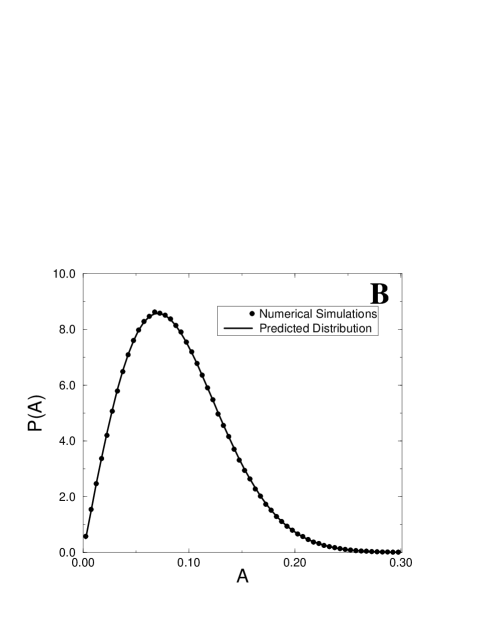
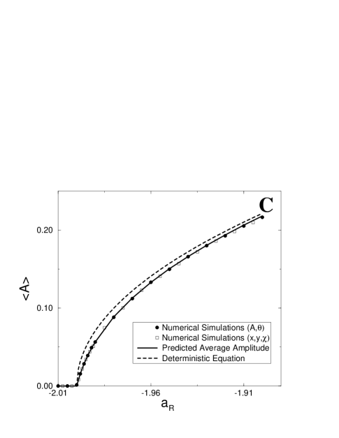
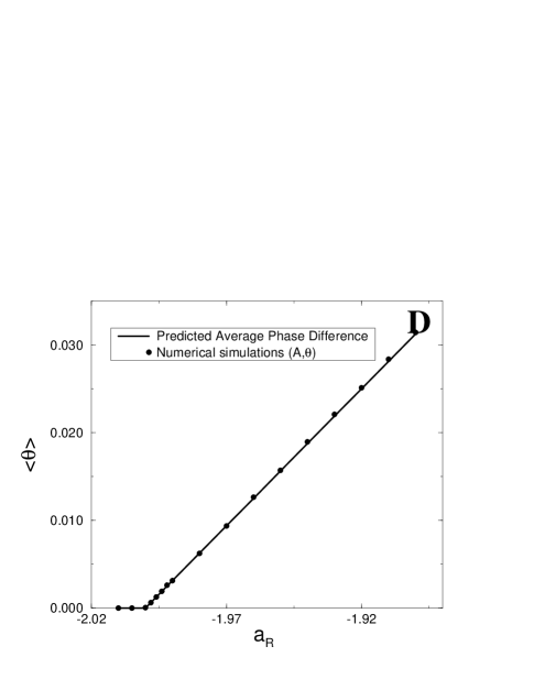
FIG. 2.: $A$ and $B$: probability distribution for the standing wave’s amplitude above onset for the same values of the parameters as in Fig 1, and, $A$, $a_{R}=-1.995$; $B$, $a_{R}=-1.98$. $C$ and $D$: average amplitude $\langle A\rangle$ and phase difference $\langle\theta\rangle$ as a function of the average control parameter $a_{R}$.

FIG. 3.: Probability distribution ${\cal P}(\chi)$ corresponding to the average modulation $b=2.25$. The distribution has a minimum at some value $\chi_{m}$ above which it starts increasing again and eventually diverges at $\chi=\pi$ (inset).

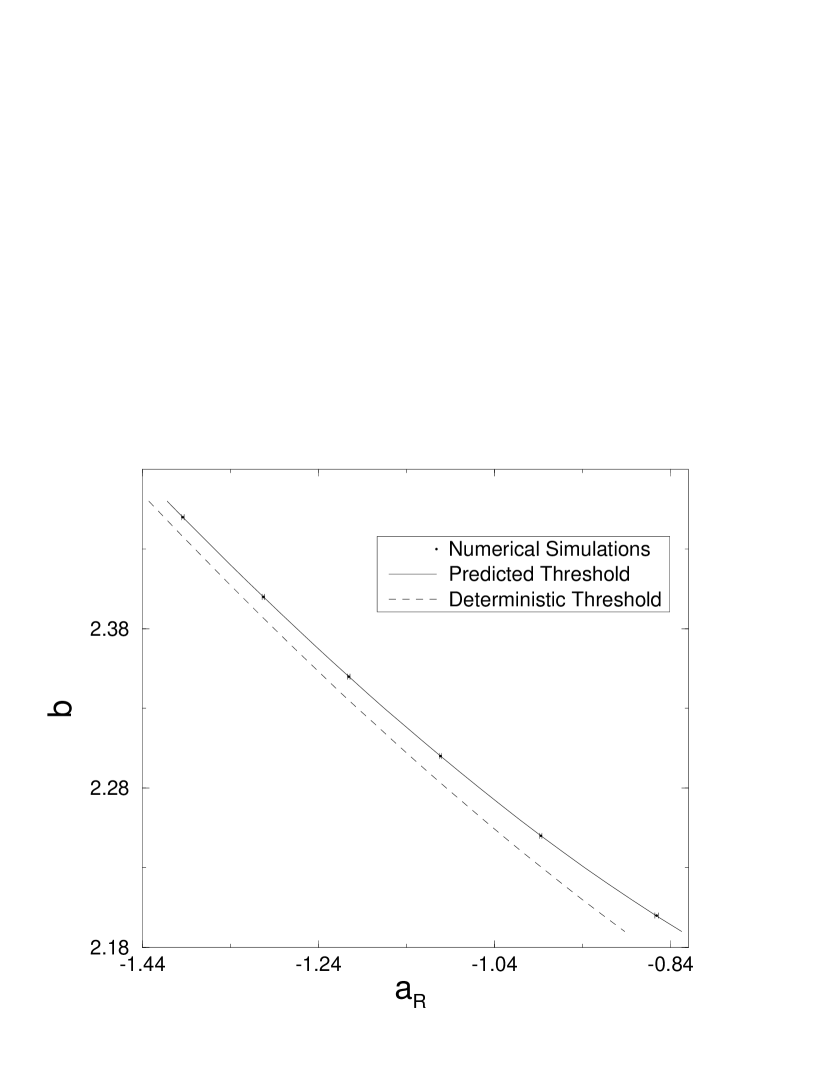
FIG. 4.: Location of onset in the presence of a fluctuating modulation amplitude $b$. For the average driving intensities shown, the bifurcation point is shifted to the right of its deterministic position.

FIG. 5.: Temporal evolution of the phase difference $\chi$ during a typical run at $b=2.25$.

REFERENCES

- [1] M. Cross and P. Hohenberg, Rev. Mod. Phys. 65, 851 (1993).
- [2] R. Clever, G. Schubert, and F. Busse, Phys. Fluids A 5, 2430 (1993).
- [3] B. Saunders et al., Phys. Fluids A 4, 1176 (1992).
- [4] P. Kolodner, D. Bensimon, and C. Surko, Phys. Rev. Lett. 60, 1723 (1988).
- [5] A. Predtechensky et al., Phys. Rev. Lett. 72, 218 (1994).
- [6] I. Rehberg et al., Phys. Rev. Lett. 61, 2449 (1988).
- [7] H. Riecke, J. Crawford, and E. Knobloch, Phys. Rev. Lett. 61, 1942 (1988).
- [8] Fluid Sciences and Materials Sciences in Space, edited by H. Walter (Springer Verlag, New York, 1987).
- [9] Low-Gravity Fluid Dynamics and Transport Phenomena, Vol. 130 of Progress in Aeronautics and Astronautics, edited by J. Koster and R. Sani (AIAA, Washington, 1990).
- [10] J. Alexander, Microgravity sci. technol. 3, 52 (1990).
- [11] J. Thomson, J. Casademunt, F. Drolet, and J. Viñals, Phys. Fluids (1997).
- [12] in Low-Gravity Fluid Dynamics and Transport Phenomena, Vol. 130 of Progress in Aeronautics and Astronautics, edited by J. Koster and R. Sani (AIAA, Washington, 1990), p. 369.
- [13] R. Graham, Phys. Rev. A 25, 3234 (1982).
- [14] M. Rodriguez, L. Pesquera, M. S. Miguel, and J. Sancho, J. Stat. Phys. 40, 669 (1985).
- [15] W. Horsthemke and R. Lefever, Noise induced transitions (Springer, New York, 1983).
- [16] L. Pesquera and M. Rodriguez, Stochastic processes applied to Physics (World Scientific, Singapore, 1985).
- [17] E. Knobloch and K. Wiesenfeld, J. Stat. Phys. 33, 611 (1983).
- [18] C. Gardiner, Handbook of Stochastic Methods for Physics, Chemistry and Natural Sciences (Springer Verlag, New York, 1985).
- [19] J. Sancho, M. S. Miguel, S. Katz, and J. Gunton, Phys. Rev. A 26, 1589 (1982).
- [20] N. Rao, J. Borwankar, and D. Ramkrishna, SIAM J. Control 12, 124 (1974).