Direct Transition to Spatiotemporal Chaos in Low Prandtl Number Fluids

Abstract

We present a large scale numerical simulation of three-dimensional Rayleigh-Bénard convection near onset, under free-free boundary conditions for a fluid of Prandtl number $\sigma=0.5$. We find that a spatiotemporally chaotic state emerges immediately above onset, which we investigate as a function of the reduced control parameter. We conclude that the transition from conduction to spatiotemporal chaos is second order and of “mean field” character. We also present a simple theory for the time-averaged convective current. Finally, we show that the time-averaged structure factor satisfies a scaling behavior with respect to the correlation length near onset.

Pattern formation in non-equilibrium systems has become a major frontier area in science [1, 2]. The richness of this field has been significantly enhanced by the existence of spatiotemporal chaos (STC) in various systems [1, 2, 3, 4, 5, 6, 7]. STC is characterized by its extensive, irregular dynamics in both space and time. It has been recognized in experiments [2, 3, 4] and numerical studies [1, 5, 6] that a large aspect ratio is essential for the occurrence of STC. Owing to the generic complication of its dynamics, theoretical understanding of STC relies heavily on some much simplified, mathematical models of the real systems [1]. Although much progress has been made, some fundamental concepts remain to be developed.

A paradigm of pattern formation is Rayleigh-Bénard convection (RBC) [2], which occurs when a thin horizontal fluid layer is heated from below. In general, the dynamics of RBC depends on the Rayleigh number $R$, the Prandtl number $\sigma$ of the fluid, and the aspect ratio (size/thickness) $\Gamma$ of the system. Busse and his collaborators [8] have studied extensively the stability domain of parallel rolls as a function of wavenumber $k$ and Rayleigh number $R$, for various $\sigma$. It is well known that in a laterally infinite system with rigid-rigid boundaries, there exists a stable, time independent parallel roll state near the onset of convection for all $\sigma$. In the case of free-free boundaries at sufficiently low Prandtl numbers ($\sigma<$0.543), Siggia and Zippelius [9] and Busse and Bolton [10] found surprisingly that parallel rolls are unstable with respect to the skewed-varicose instability immediately above onset. Busse et al. [11] further studied the possibility of a direction transition from conduction to STC, but their aspect ratio ($\Gamma=8$) is not large enough for a conclusive result. Although the free-free boundaries are very difficult to control for detailed experimental studies, one experiment with such boundary conditions has been reported [12].

In this paper, we present the results of a large scale ($\Gamma=60$) numerical simulation of the three dimensional hydrodynamic equations, using the Boussinesq approximation, for a low Prandtl number fluid ($\sigma$=0.5) with free-free boundary conditions. The same problem has been investigated before [11, 13], but the aspect ratio used by previous studies is too small for the occurrence of STC. We find from our extensive numerical simulation that the convective state just above onset is spatiotemporally chaotic, which is evident from the snapshot images of the vertical velocity field and from the dynamical behavior of three important global quantities: the viscous dissipation energy, the thermal dissipation energy and the work done by the buoyancy force. This thus provides another example of a direct transition to STC, in addition to the Küppers-Lortz transition [4, 14], ac driven electroconvection and a few others [7]. Our method suggests that by studying the dynamical behavior of some global quantities of systems which exhibit STC, one may obtain valuable information about the temporal chaos of these systems. We also measure the fractal dimensions of the global quantities and find a value of about $1.4$. In addition, we investigate the nature of the conduction to STC transition, as well as certain properties of the spatiotemporally chaotic state. Our results for the correlation length suggest that the transition is second order, with a mean field power law behavior. In comparison recent experimental results for the Küppers-Lortz transition are not consistent with a mean field power law behavior [4]. We present below a simple but rather accurate theory for the behavior of the time-averaged convective current as a function of the reduced control parameter. Finally, we show that the time-averaged structure factor (power spectrum) exhibits a scaling behavior with respect to the correlation length similar to that found in critical phenomena.

The Boussinesq equations, which describe the evolution of the velocity field $\vec{u}(x,y,z,t)=(u,v,w)$ and the deviation of the temperature field $\theta(x,y,z,t)$ from the conductive profile, can be written in dimensionless form as

$$\left\{\begin{array}[]{lll}\nabla\cdot\vec{u}=0,\\ \partial\vec{u}/\partial t+(\vec{u}\cdot\nabla)\vec{u}=-\nabla p+\sigma\theta\vec{e}_{z}+\sigma\nabla^{2}\vec{u},\\ \partial\theta/\partial t+\vec{u}\cdot\nabla\theta=\nabla^{2}\theta+wR,\end{array}\right.$$ (1)

where $\vec{e}_{z}$ is the unit vector in the vertical z-direction. In the idealized limit of a laterally infinite system, the critical Rayleigh number $R_{c}=27\pi^{4}/4$ and the onset wavenumber $k_{c}=\pi/\sqrt{2}$. The efficient Marker-and-Cell (MAC) [15, 16] numerical technique is employed. (In developing our algorithm, we have carried out two tests: One is against the theoretical results of Schlüter et al. [17]; the other is against the numerical results of Kirchartz and Oertel [18]. In both cases agreements within $1\%$ have been found.) The boundary conditions for the velocities $\vec{u}$ are free-slip at the upper and lower surfaces, and no-slip at the sidewalls. The temperature deviation $\theta$ is zero on the top and bottom surfaces, while the temperature gradient $\nabla\theta$ normal to the sidewall is set to zero. For the initial conditions of $\vec{u}$ and $\theta$, we have tried both random values and values of Gaussian distribution, inside a possible range. Since no difference has been found, the actual calculation is carried out with initial conditions of Gaussian distribution. Our parameters are $\sigma=0.5$ and $0.03\leq\epsilon\leq 0.5$, where $\epsilon=(R-R_{c})/R_{c}$ is the reduced Rayleigh number. We use mesh points N${}_{x}\times$ N${}_{y}\times$ N_z =256 $\times$ 256 $\times$18 and a grid size $\Delta x$=$\Delta y$=60/256, $\Delta z$=1/18 for an aspect ratio $\Gamma$ =60 in the simulation. We have run for $360$ vertical diffusion times before collecting data. Considering that the normal relaxation time to approach a steady state is about $10$ vertical diffusion times [$\tau_{relax}=2(1+\sigma)/3\pi^{2}\sigma\epsilon$], we believe that we are well beyond any transient regime.

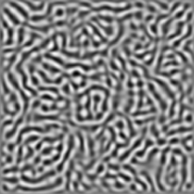
FIG. 1.: A typical image of the spatially disorganized pattern in the cell. Dark regions correspond to hot rising fluid and white regions correspond to cold descending fluid. The vertical velocity field $w$(x,y,z=1/2) for $\epsilon=0.1$ is shown here.

For the low Prandtl number fluid studied here, the convective pattern near onset has an irregular space-time dependence. In Figure 1 we show a snap shot image of the vertical velocity field $w(x,y,z=1/2)$ from the numerical simulation at $\epsilon=0.1$. In this image, the apparently disorganized spatial pattern consists of superimposed rolls with many different orientations. The time evolution of these rolls is through an interface motion, which maintains the type of spatial disorder shown in Figure 1. Similar images are found for other values of $\epsilon$. It is obvious from such images that the convection pattern near onset is random in space.

To illustrate the temporal chaos of the system, we now investigate the dynamics of the global quantities which characterize the underlying physics of Rayleigh-Bénard convection. Using $\langle f\rangle$ to denote the average of $f$ over the whole system and taking into account the boundary conditions as well as the incompressibility condition, we obtain $\frac{1}{2}d\langle\vec{u}\cdot\vec{u}\rangle/dt=F_{2}(t)-F_{1}(t)$, and $\frac{1}{2}d\langle\theta^{2}\rangle/dt=F_{4}(t)-F_{3}(t)$, where (a) $F_{1}=\frac{1}{2}\sigma\langle(\partial u_{i}/\partial x_{j}+\partial u_{j}/\partial x_{i})^{2}\rangle$ is the kinetic energy dissipated by the viscosity; (b) $F_{2}=\sigma\langle w\theta\rangle$ is the work done by the buoyancy force; (c) $F_{3}=\langle\nabla\theta\cdot\nabla\theta\rangle$ is the dissipative thermal energy (generation of entropy) owing to temperature fluctuations; and (d) $F_{4}=R\langle w\theta\rangle=(RF_{2}/\sigma)$ is the flow of the entropy fluctuations carried by the vertical velocity. It is clear that in the special case of steady state ($\frac{\partial}{\partial t}=0$), one recovers the condition $F_{1}=F_{2}$ and $F_{4}=F_{3}$. These global quantities provide us with a complete description of “energy-balance” in the Rayleigh-Bénard system.

FIG. 2.: A plot of global quantities $F_{1}(t)$, $F_{2}(t)$ and $F_{3}(t)$ as functions of time for $\epsilon=0.2$. Note that they lie on top of each other with differences, though substantial, too small to be seen. The time is in units of vertical thermal diffusion time $t_{v}=d^{2}/\kappa$ and the origin corresponds to $t=330t_{v}$ in real calculation.

We plot a representative time series of these quantities, $F_{1}(t)$, $F_{2}(t)$ and $F_{3}(t)$, in Figure 2 for $\epsilon=0.2$. We have rescaled $F_{1}$, $F_{2}$ by $\sigma R_{c}$, and $F_{3}$ by $RR_{c}$ so that we have $F_{1}=F_{2}=F_{3}$ in a steady state. (Note that $F_{4}$ is simply related to $F_{2}$ by the factor R/$\sigma$.) The most important implication of this figure is the apparent chaotic behavior of these quantities over the time interval that is accessible to us. To be more concrete, we apply the Grassberger and Procaccia method [19] to compute the fractal dimensions $D_{f}$ for these quantities and find $D_{f}=1.42\pm 0.02$. This of course is different from the fractal dimension that is normally used to characterize STC, which diverges with the system size. We believe that such global quantities might provide a relatively simple way to characterize the temporally chaotic nature of spatiotemporally chaotic states such as studied here, although data over a longer time interval will be necessary for such an analysis. It is also interesting to observe that the dynamics of these three quantities are almost exactly the same, i.e. $F_{1}(t)\simeq F_{2}(t)\simeq F_{3}(t)$, as shown in Figure 2. Although the differences among them are substantial and beyond numerical uncertainties, they are too small to be seen under the scale of Figure 2. In fact, this is the case for all $\epsilon$ studied in the range $0.03\leq\epsilon\leq 0.5$. This is certainly a surprising result considering the irregular spatiotemporal state we observed. However, a theoretical understanding of this has been obtained, as outlined later. This result also implies that the quantity $\Re=\sigma F_{3}/(2F_{2}-F_{1})$, which is often used as a variational formulation to determine the critical Rayleigh number, behaves as if the system is almost in a steady state.

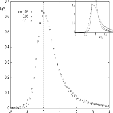
FIG. 3.: A plot of $kS(k)/\xi$ vs $x=(k-k_{max})\xi$ (in units of $k_{c}$), showing scaling and the scaling function F(x) defined in the text. Insert: The time-averaged function $kS(k)$ vs. $k/k_{c}$ for $\epsilon=0.03$, $0.05$ and $0.1$.

In order to gain more insight into the nature of the transition to STC near onset, we have studied the two-dimensional structure factor (Fourier power spectrum). Since the snapshot images of the patterns appears to be isotropic azimuthally, we calculate the azimuthally averaged structure factor, and then average the images over time, to obtain the time-averaged structure factor $S(k)$. The function $kS(k)$ is shown for several different values of $\epsilon$ in the insert in Figure 3. We also show in this figure that $kS(k)$ satisfies a scaling behavior somewhat similar to that found in critical phenomena, namely, $kS(k)/\xi=F[(k-k_{max})\xi]$, where $\xi$ is the correlation length (defined below) and where we have normalized the integral of $S(k)$ over $k$-space to be unity. Here $k_{max}$ is the wavenumber which maximizes $kS(k)$, which we choose to give the best fit to scaling. Another interesting feature of the structure factor is associated with the power-law behavior of S(k) $\sim k^{-3}$ for large wavenumber. This feature is observed over the range of $\epsilon$ studied here. It is interesting to note that this is the same power-law behavior observed in phase separating systems, in two dimensions, where it is known as Porod’s law. In both cases it results from the linear behavior of the real space correlation function, C(r), for small r, where this correlation function is the azimuthal average of the inverse Fourier transform of the structure factor.

FIG. 4.: A plot of $\xi^{-2}$ vs. $\epsilon$. The vertical bars indicate the standard deviation, and the solid line corresponds to $\xi^{-2}=\xi_{0}^{-2}\epsilon$ with $\xi_{0}=0.78$. These data can also be fitted with a nonconventional exponent: see the text for more detail.

We have also calculated the correlation length $\xi$ as a function of the control parameter $\epsilon$, where we define the correlation length through the variance of the wavenumber, i.e. $\xi=(\overline{k^{2}}-\overline{k}^{2})^{-1/2}$. The moment $\overline{k^{n}}$ is defined as $\overline{k^{n}}=\int|\vec{k}|^{n}S(\vec{k})d^{2}\vec{k}/\int S(\vec{k})d^{2}\vec{k}$ and $S(\vec{k})$ is the time-averaged structure factor. We find that the correlation length $\xi$ appears to diverge as $\epsilon$ approaches the transition point, with a power-law behavior of $\xi=\xi_{0}(\epsilon-\epsilon_{c})^{-\nu}$ with $\nu=0.472\pm 0.016$, $\xi_{0}=0.82\pm 0.04$ and $\epsilon_{c}=0.005$. (The fact that $\epsilon_{c}$ is finite instead of zero is due to finite size effects.) The behavior of the correlation length is also consistent with a mean field power low exponent of $\nu=0.5$ and $\xi_{0}=0.78$. This is illustrated in Figure 4. The amplitude value $\xi_{0}$ is a factor of $3/2$ larger than the value $\xi_{0}=\sqrt{8/3\pi^{2}}=0.52$ calculated from the curvature of the marginal stability curve.

In order to investigate the heat transport in STC near onset, we calculate the Nusselt number $N(t)=1+\langle w\theta\rangle/R$, which describes the ratio between the heat transport with and without convection, as a function of $\epsilon$. The quantity $N-1$ can be fit with a power law behavior of the form $N-1=(\epsilon-\epsilon_{c})^{\mu}/\overline{g}$ with $\mu=1.034\pm 0.025$, $\epsilon_{c}=0.012$ and $\overline{g}=1.27\pm 0.03$. Figure 5 shows that the time-averaged $N-1$ is also consistent with a linear relation $(\epsilon-\epsilon_{c})/\overline{g}$, where $\epsilon_{c}=0.01$ and $\overline{g}=1.23$. (Again, owing to finite size effects, the value of $\epsilon_{c}$ is nonzero.) We have also determined the time-averaged vertical “vortex energy” $\Omega=\langle\omega_{z}^{2}\rangle$, where $\omega_{z}$ is the vertical vorticity, as a function of $\epsilon$ from our simulations and observed a power-law behavior of $\Omega\sim\epsilon^{\lambda}$ with $\lambda=5/2$.

FIG. 5.: Time-averaged $N-1$ vs $\epsilon$ near onset. The vertical bars indicate the standard deviation, and the solid line is the fit of $(\epsilon-\epsilon_{c})/\overline{g}$ to the data with $\epsilon_{c}=0.01$ and $\overline{g}=1.23$. A slightly different fitting form is given in the text.

For theoretical understanding of some of our results, we notice that the velocity $\vec{u}$ and the temperature derivation $\theta$ near onset can be approximated by an order parameter $\psi(\vec{r})$ in two-dimensional space $\vec{r}$ multiplied by known prefactors with $z$-dependence [20]. It is then straightforward to rewrite the global quantities $F_{1}$, $F_{2}$ and $F_{3}$, and the Nusselt number $N$ in terms of $\psi(\vec{r})$. We further assume that only those modes inside the vicinity of $k_{c}$ are excited and equally excited. From these approximations, we confirm (after rescaling mentioned earlier) that $F_{1}(t)\simeq F_{2}(t)\simeq F_{3}(t)$. We also obtain that

$$\overline{g} = g(-1)+(2/\pi)\int_{0}^{\pi}g(\cos\alpha)d\alpha$$ (2)

$$= 0.855951+0.0458145\sigma^{-1}+0.0709325\sigma^{-2},$$ (3)

where $\alpha$ is the angle between $\vec{k}$ and some reference direction, and we have used the explicit form of $g(\cos\alpha)$ given by Schlüter et al. [17] for free-free boundary conditions [20]. For $\sigma$=0.5, we find $\overline{g}$= 1.2313, which is in surprisingly good agreement with the numerical results. The theory of the vortex energy $\Omega\sim\epsilon^{5/2}$ is more complicated than the above. All this theoretical analysis will be presented elsewhere.

In summary, we have presented a large scale numerical simulation of pattern formation in three dimensional Rayleigh-Bénard convection. We have calculated the spatial correlation length and the Nusselt number as a function of the reduced control parameter, as well as the dynamics of the viscous energy, the dissipative thermal energy and the work done by the buoyancy force. Our numerical studies suggest that the transition from the conduction state to spatiotemporal chaotic state near onset is a continuous (second order) transition, with mean field exponents for the correlation length and the time-averaged convective current. We have also demonstrated that the time-averaged structure factor satisfies a scaling behavior with respect to the correlation length. We believe that more studies of scaling in STC by systematic experiments for smaller $\epsilon$, larger aspect ratio, and with both free-free and rigid-rigid boundary conditions will be challenging and valuable.

X.J.L. and J.D.G. are grateful to the National Science Foundation for support under Grant No. DMR-9596202. The computations were performed at the Pittsburgh Supercomputing Center and the Ohio Supercomputer Center.

REFERENCES

- [1] M. C. Cross and P. C. Hohenberg, Rev. Mod. Phys. 65, 851 (1993) and references therein.
- [2] G. Ahlers, Over Two Decades of Pattern Formation, a Personal Perspective [preprint].
- [3] S. W. Morris, E. Bodenschatz, D. S. Cannell and G. Ahlers, Phys. Rev. Lett. 71, 2026 (1993); Y. Hu, R. E. Ecke and G. Ahlers, ibid 74, 391 (1995).
- [4] Y. Hu, R. E. Ecke and G. Alhers, Phys. Rev. Lett. 74, 5040 (1995).
- [5] H.-W. Xi, J. D. Gunton and J. Viñals, Phys. Rev. Lett. 71, 2030 (1993); H.-W. Xi and J. D. Gunton, Phys. Rev. E 52, 4963 (1995).
- [6] W. Decker, W. Pesch and A. Weber, Phys. Rev. Lett. 73, 648 (1994).
- [7] A. G. Rossberg, A. Hertrich, L. Kramer and W. Pesch, Phys. Rev. Lett. 76, 4729 (1996) and references therein.
- [8] F. H. Busse, Rep. Prog. Phys. 41, 1929 (1978).
- [9] A. Zippelius and E. D. Siggia, Phys. Rev. A 26, 1788 (1982); Phys. Fluids 26, 2905 (1983).
- [10] F. H. Busse and E. W. Bolton, J. Fluid Mech. 146, 115 (1984); E. W. Bolton and F. H. Busse, ibid 150 487 (1985).
- [11] F. H. Busse, M. Kropp, and M. Zaks, Physica D 61, 94 (1992). The aspect ratio used is .
- [12] R. J. Goldstein and D. J. Graham, Phys. Fluids 12, 1133 (1969).
- [13] W. Arter, J. Fluid Mech. 152, 391 (1985); M. Meneguzzi et al., ibid 182, 169 (1987). The aspect ratio used by these authors is for the first and for the second.
- [14] G. Küppers and D. Lortz, J. Fluid Mech. 35, 609 (1969); G. Küppers, Phys. Lett. A 32, 7 (1970).
- [15] F. H. Harlow and J. E. Welch, Phys. Fluids 8, 2182 (1965).
- [16] B. D. Nichols, C. W. Hirt, and R. S. Hotchkiss, Los Alamos Scientific Lab. Rep. LA-8355 (1989).
- [17] A. Schlüter, D. Lortz, and F. Busse, J. Fluid Mech. 23, 129 (1965).
- [18] K. R. Kirchartz and H. Oertel, Jr., J. Fluid Mech. 192, 249 (1988).
- [19] P. Grassberger and I. Procaccia, Phys. Rev. Lett. 50, 346 (1983).
- [20] M. C. Cross, Phys Fluids 23, 1727 (1980).