EXTENDED SYMBOLIC DYNAMICS IN BISTABLE CML: EXISTENCE AND STABILITY OF FRONTS

Ricardo COUTINHO and Bastien FERNANDEZ

Abstract

We consider a diffusive Coupled Map Lattice (CML) for which the local map is piece-wise affine and has two stable fixed points. By introducing a spatio-temporal coding, we prove the one-to-one correspondence between the set of global orbits and the set of admissible codes. This relationship is applied to the study of the (uniform) fronts’ dynamics. It is shown that, for any given velocity in $[-1,1]$, there is a parameter set for which the fronts with that velocity exist and their shape is unique. The dependence of the velocity of the fronts on the local map’s discontinuity is proved to be a Devil’s staircase. Moreover, the linear stability of the global orbits which do not reach the discontinuity follows directly from our simple map. For the fronts, this statement is improved and as a consequence, the velocity of all the propagating interfaces is computed for any parameter. The fronts are shown to be also nonlinearly stable under some restrictions on the parameters. Actually, these restrictions follow from the co-existence of uniform fronts and non-uniformly travelling fronts for strong coupling. Finally, these results are extended to some $C^{\infty}$ local maps.

Key Words: Coupled Map Lattices, Symbolic Dynamics, Fronts.

Number of figures: 2

June 1996

Submitted to Physica D

1 Introduction

The occurrence of interfaces is a very common phenomenon in extended systems out of equilibrium. These patterns appear, in systems with many equilibrium states, as solutions linking two different equilibria, namely two phases [1]. When the time evolution of the system shows the motion of an interface resulting in an invasion of one phase into the other, the phenomenon under consideration is usually called a front. These structures arise in various experimental systems such as reaction-diffusion chemical systems [2], alloy solidification [3] and crystal growth [4].

From a mathematical point of view, the description of the front dynamics using space-time continuous models is now complete, at least for several one-dimensional Partial Differential Equations [5]. Also, in discrete space and continuous time systems, i.e. in Ordinary Differential Equations, the dynamics of these interfaces is well understood [6, 7]. However, in space-time discrete models such as the Coupled Map Lattice (CML), the study is not as complete; except for the one-way coupled model [9]. CML’s have been proposed as the simplest models of space-time discrete dynamics with continuous states and they serve now as a paradigm in the framework of nonlinear extended dynamical systems [10].

The phenomenology of the interface dynamics differs between discrete space and continuous space systems. In the former case, varying the coupling strength induces a bifurcation from a regime of standing interfaces to a regime of fronts in which the propagation can be interpreted as a mode-locking phenomenon [6, 9]. These effects are assigned to the discreteness of space and are well-known in solid-state physics [11].

In previous studies of the piece-wise affine bistable CML, the problem of steady interfaces was solved and the fronts’ structure was thoroughly investigated by means of generalized transfer matrices [12, 13]. Nevertheless, this technique did not allowed us to prove the existence of fronts of any velocity, nor to understand clearly their dependence on the parameters, in particular that of the fronts’ velocity.

In the same CML, using techniques employed for the piece-wise linear mappings [14, 15], we now prove the one-to-one correspondence between the set of orbits that are defined for all times, i.e. the global orbits, and a set of spatio-temporal codes (Section 2 and 3). Our model is locally a contraction, hence these orbits are shown to be linearly stable when they never reach the local map’s discontinuity (Section 4). Further, using the orbit-code correspondence, the existence of fronts is stated and their velocity is computed (Section 5). In Section 6, the linear stability of fronts with rational velocity is given for a large class of initial conditions. In the following, we study the dynamics of the propagating interfaces. In particular, their velocity is computed for all the parameters (Section 7). Using these results, the nonlinear stability, i.e. the stability of fronts with respect to any kink initial condition, is proved in Section 8 using a method similar to the Comparison Theorem [5]. This result holds for any rational velocity provided the coupling is small enough. We justify such a restriction by the existence of non-uniform fronts for large coupling which co-exist with the fronts. Finally, some concluding remarks are made, in particular we emphasize the extension of these results to certain $C^{\infty}$ local maps.

2 The CML and the associated coding

Let $M\in{{R}}$ be fixed and ${\cal M}=[-M,M]^{{{Z}}}$ be the phase space of the CML under consideration. The CML is the one-parameter family of maps

$$\begin{array}[]{rl}F_{\epsilon}:&{\cal M}\longrightarrow{\cal M}\\ &x^{t}\longmapsto x^{t+1},\end{array}$$

where $x^{t}=\left\{x_{s}^{t}\right\}_{s\in{{Z}}}$ is the state of the system at time $t$. This model is required to be representative of the reaction-diffusion dynamics. Therefore the new state at time $t+1$ is given by [10]:

$$x_{s}^{t+1}\equiv(F_{\epsilon}x^{t})_{s}=(1-\epsilon)f(x_{s}^{t})+{\epsilon\over 2}\left(f(x_{s-1}^{t})+f(x_{s+1}^{t})\right)\quad\forall s\in{{Z}}.$$ (1)

Here the coupling strength $\epsilon\in(0,1]$ and we choose the local map $f$ to be bistable and piece-wise affine [13]:

$$f(x)=\left\{\begin{array}[]{ccc}ax+(1-a)X_{1}&if&x<c\\ ax+(1-a)X_{2}&if&x\mathchar 13374\relax c,\end{array}\right.$$

where $a\in(0,1)$ and $-M\mathchar 13366\relax X_{1}<c\mathchar 13366\relax X_{2}\mathchar 13366\relax M$. These conditions ensure the existence of the two stable fixed points $X_{1}$ and $X_{2}$, the only attractors for $f$.

This local map reproduces qualitatively the autocatalytic reaction in chemical systems [2], or the local force applied to the system’s phase in the process of solidification [3].

For the sake of simplicity we assume $X_{1}=0$ and $X_{2}=1$. This is always possible by a linear transformation of the variable.

For a state $x^{t}$, the sequence $\theta^{t}=\left\{\theta_{s}^{t}\right\}_{s\in{{Z}}}\$ defined by

$$\theta_{s}^{t}=\left\{\begin{array}[]{ccc}0&if&x_{s}^{t}<c\\ 1&if&x_{s}^{t}\mathchar 13374\relax c,\end{array}\right.$$

is called the spatio-temporal code or the code unless it is ambiguous.

3 The orbit-code correspondence

The study of the orbits, in particular those that exist for all the times $t\in{{Z}}$, can be achieved using their code. In this section, we first compute explicitly the positive orbits for any initial condition. Then we prove the one-to-one correspondence between the global orbits and their code.

Notice that the local map can be expressed in terms of the code

$$f(x_{s}^{t})=ax_{s}^{t}+(1-a)\theta_{s}^{t}.$$

By introducing this expression into the CML dynamics, one obtains a linear non-homogeneous finite-difference equation for $x_{s}^{t}$ in which the code only appears in the non-homogeneous term. Using the Green functions’ method, this equation may be solved and the solution, as a function of the code $\left\{\theta_{s}^{k}\right\}_{s\in{{Z}},t_{0}\mathchar 13366\relax k\mathchar 13366\relax t-1}$ and of the initial condition $\{x_{s}^{t_{0}}\}_{s\in{{Z}}}$, is given by

$$x_{s}^{t}=\sum_{k=1}^{t-t_{0}}\sum_{n=-k}^{k}l_{n,k}\theta_{s-n}^{t-k}+{a\over 1-a}\sum_{n=-(t-t_{0})}^{t-t_{0}}l_{n,t-t_{0}}x_{s-n}^{t_{0}}\quad\forall t>t_{0}\ {\rm and}\ s\in{{Z}},$$ (2)

where the coefficients $l_{n,k}$ satisfy the recursive relations

$$l_{n,k}=(1-a)\delta_{1,k}\left((1-\epsilon)\delta_{n,0}+{\epsilon\over 2}(\delta_{n,1}+\delta_{n,-1})\right)\quad\forall n\in{{Z}}\ {\rm and}\ k\mathchar 13366\relax 1,$$

and

$$l_{n,k+1}-a(1-\epsilon)l_{n,k}-{a\epsilon\over 2}\left(l_{n+1,k}+l_{n-1,k}\right)=0\quad\forall n\in{{Z}}\ {\rm and}\ k\mathchar 13374\relax 1.$$

From the latter, it follows that for $\epsilon\in(0,1)$

$$l_{n,k}=0\quad{\rm iff}\quad|n|>k\ {\rm or}\ n=k=0,$$

and, one can derive the bounds

$$0\mathchar 13366\relax l_{n,k}\mathchar 13366\relax(1-a)a^{k-1},$$ (3)

and the normalization condition

$$\sum_{n,k\in{{Z}}}l_{n,k}=1.$$

Further properties of these coefficients are given in Appendix A.

The study is now restricted to the global orbits $\{x^{t}\}_{t\in{{Z}}}$. That is to say, we consider the sequences which belong to

$$\Lambda=\left\{\{x^{t}\}_{t\in{{Z}}}\in{\cal M}^{{{Z}}}\ :\ F_{\epsilon}(x^{t})=x^{t+1}\ \forall t\in{{Z}}\right\}.$$

For such orbits, taking the limit $t_{0}\rightarrow-\infty$ and using the bounds (3) in (2) leads to the relation:

$$x_{s}^{t}=\sum_{k=1}^{+\infty}\sum_{n=-k}^{k}l_{n,k}\theta_{s-n}^{t-k}\quad\forall s,t\in{{Z}},$$ (4)

which gives the correspondence between these orbits and their code as we state now.

By the relation (4), all the orbits in $\Lambda$ stay in $[0,1]^{{{Z}}}$. Hence their code can be uniquely computed by

$$\theta_{s}^{t}=\lfloor x_{s}^{t}-c\rfloor+1\quad\forall s,t\in{{Z}},$$ (5)

where $\lfloor.\rfloor$ stands for the floor function.

From (4) and (5) it follows that for any orbit in $\Lambda$, its code must obey the following relation:

$$c-1\mathchar 13366\relax\sum_{k=1}^{+\infty}\sum_{n=-k}^{k}l_{n,k}\left(\theta_{s-n}^{t-k}-\theta_{s}^{t}\right)<c\quad\forall s,t\in{{Z}},$$

which is called the admissibility condition. Then, conversely to the preceding statement, for a sequence $\theta\in\{0,1\}^{{{Z}}^{2}}$ that satisfies this condition, there is a unique orbit in $\Lambda$, given by (4).

The spatio-temporal coding is an effective tool for the description of all the global orbits of the piece-wise affine bistable CML [16]. These orbits are important since they collect the physical phenomenology of our model.

4 The linear stability of the global orbits

We prove in this section the stability of the orbits in $\Lambda$ with respect to small initial perturbations. Let the norm

$$\|x\|=\sup_{s\in{{Z}}}|x_{s}|,$$

for $x\in{\cal M}$ and

$$\left({\rm L}x\right)_{s}=a\left((1-\epsilon)x_{s}+{\epsilon\over 2}(x_{s+1}+x_{s-1})\right)\quad\forall s\in{{Z}},$$

be the CML linear component. Notice that ${\rm L}$ is invertible on ${\cal M}$ if $\epsilon<{1\over 2}$ and

$$\|{\rm L}\|=\sup_{x\neq 0}{\|{\rm L}x\|\over\|x\|}=a.$$

The linear stability is claimed in

Proposition 4.1

Let $\left\{x^{t}\right\}_{t\in{{N}}}$ be an orbit such that

$$\exists\delta>0\ :\ |x_{s}^{t}-c|>\delta a^{t}\quad\forall t\mathchar 13374\relax 0,\ s\in{{Z}}.$$

Then for any initial condition $y^{0}$ in a neighborhood of $x^{0}$, i.e.

$$\|y^{0}-x^{0}\|<\delta,$$

we have

$$\|y^{t}-x^{t}\|<\delta a^{t}\quad\forall t\mathchar 13374\relax 0.$$

Equivalently, $x^{t}$ and $y^{t}$ have the same code for all times.

Proof: The relation (1) with the present local map can be written in terms of the operator ${\rm L}$

$$x^{t+1}={\rm L}x^{t}+{1-a\over a}{\rm L}\theta^{t}$$ (6)

where $\theta^{t}=\{\theta_{s}^{t}\}_{s\in{{Z}}}$ is the code of $x^{t}$. Using this relation, one shows by induction that the codes of the two orbits remains equal for all the times; also using (6), the latter implies the statement. $\Box$

Notice that this assertion is effective for the orbits in $\Lambda$ that never reach $c$, since in this situation $\delta$ can be computed (see Proposition 6.1 below for the case of fronts). Further, because our system is deterministic, when this proposition holds for an orbit $\{x^{t}\}$ and a given initial condition $y$, it cannot hold for a different orbit $\{\tilde{x}^{t}\}$ and the same initial condition $y$, unless both these orbits converge to each other. Hence, using this statement, one may be able to determine the (local) basin of attraction for any orbit in $\Lambda$ that never reaches $c$.

5 The existence of fronts

We now apply the orbit-code correspondence to a particular class of travelling wave orbits, namely the fronts.

Definition 5.1

A front with velocity $v$ is an orbit in $\Lambda$ given by

$$x_{s}^{t}=\phi(s-vt-\sigma)\quad\forall s,t\in{{Z}},$$

where $\sigma\in{{R}}$ is fixed and, the front shape $\phi:{{R}}\longrightarrow{{R}}$, is a right continuous function which obey the conditions

$$\left\{\begin{array}[]{ccc}\phi(x)<c&{\rm if}&x<0\\ \phi(x)\mathchar 13374\relax c&{\rm if}&x\mathchar 13374\relax 0.\end{array}\right.$$ (7)

The front shape has the following spatio-temporal behavior:

$$\lim_{x\rightarrow-\infty}\phi(x)=0\quad{\rm and}\quad\lim_{x\rightarrow+\infty}\phi(x)=1.$$

In this way, the fronts are actually the travelling interfaces as described in the introduction. Moreover, for any front shape, the front changes by varying $\sigma$; but if $v={p\over q}$ with $p$ and $q$ co-prime integers, there are only $q$ different fronts that cannot be deduced from one another by space translations. On the other hand, when $v$ is irrational, the family of such orbits becomes uncountable. (Both these claims are deduced from the proof of Theorem 5.2 below.)

The existence of fronts is stated in

Theorem 5.2

Given $(a,\epsilon)$ there is a countable nowhere dense set ${\rm G}_{a,\epsilon}\subset(0,1]$ such that, for any $c\in(0,1]\setminus{\rm G}_{a,\epsilon}$, there exists a unique front shape. The corresponding front velocity is a continuous function of the parameters with range $[-1,1]$.

In other words, for any velocity $v$, there is a parameter set for which the only fronts that exist are those of velocity $v$.

Furthermore, for $c\in{\rm G}_{a,\epsilon}$, no front exists. But, the front velocity can be extended to a continuous function for all the values of the parameters.

Referring to a similar study of a circle’s map [15], we point out that, even when no front exists, numerical simulations show convergence towards a “ghost” front. Actually, by enlarging the linear stability result, this comment is proved (see Proposition 6.3 below). A ghost front is a front-like sequence in ${\cal M^{{{Z}}}}$, that is not an orbit of the CML and, for which the (spatial) shape obeys, instead of (7), the conditions

$$\left\{\begin{array}[]{ccc}\phi(x)\mathchar 13366\relax c&{\rm if}&x<0\\ \phi(x)>c&{\rm if}&x\mathchar 13374\relax 0.\end{array}\right.$$

Ghosts fronts arise in this model because the local map is discontinuous. Moreover, given the parameters, one can avoid this ghost orbit by changing the value of the local map $f$ at $c$.

Proof of Theorem 5.2:

It follows from Definition 5.1 that if a front with velocity $v$ exists, the code associated with this front is given by

$$\theta_{s}^{t}=H(s-vt-\sigma)\quad\forall s,t\in{{Z}},$$

where $H$ is the Heaviside function. Hence by (4) the corresponding front shape has the following expression:

$$\phi(x)=\sum_{k=1}^{+\infty}\sum_{n=-k}^{k}l_{n,k}H(x-n+vk)\quad\forall x\in{{R}}.$$ (8)

Such a function is increasing (strictly if $v$ is irrational), right continuous and its discontinuity points are of the form $x=n-vk\ (k\mathchar 13374\relax 1,n\in{{Z}}$ and $|n|\mathchar 13366\relax k)$. Now one has to prove that, given $(a,\epsilon,c)$, there exists a unique front velocity such that (8) satisfy the conditions (7), i.e. there exists a unique $v$ such that the code $H(s-vt-\sigma)$ is admissible. For this let

$$\eta(a,\epsilon,v)\equiv\phi(0)=\sum_{k=1}^{+\infty}\sum_{n=-k}^{\lfloor vk\rfloor}l_{n,k},$$

where the continuous dependence on $a$ and $\epsilon$ is included in the $l_{n,k}$ which are uniformly summable. It is immediate that $\eta(a,\epsilon,v)$ is a strictly increasing ($\epsilon\neq 0$), right continuous function of $v$. Moreover, it is continuous on the irrationals and

$$\eta(a,\epsilon,{p\over q})-\eta(a,\epsilon,{p\over q}^{-})>0.$$

The conditions (7) impose that $v$ be given by

$$\bar{v}(a,\epsilon,c)=\min\left\{v\in{{R}}:\eta(a,\epsilon,v)\mathchar 13374\relax c\right\}.$$ (9)

Actually, if $\bar{v}(a,\epsilon,c)$ is irrational then

$$\phi(x)<\phi(0)=c\ {\rm if}\ x<0.$$

If $\bar{v}(a,\epsilon,c)$ is rational we have

$$\phi(x)=\phi(0^{-})=\eta(a,\epsilon,{p\over q}^{-})\ {\rm if}\ -{1\over q}\mathchar 13366\relax x<0,$$

hence either $\phi(0^{-})<c$ and the front exists, or $\phi(0^{-})=c$ and the first condition in (7) is not satisfied. In the latter case, given $(a,\epsilon)$ and $v={p\over q}$, there is a unique $c$ that realizes $\phi(0^{-})=c$. The countability of the values of $c$ for which there is no front then follows.

In this way, we can conclude that for $a,\epsilon$ and ${p\over q}$ fixed, there exists an interval of the parameter $c$ given by

$$\eta(a,\epsilon,{p\over q}^{-})<c\mathchar 13366\relax\eta(a,\epsilon,{p\over q}),$$

for which the front shape uniquely exists and the front velocity is $\bar{v}(a,\epsilon,c)={p\over q}$. Moreover, we have

$${\rm G}_{a,\epsilon}=\left\{\eta(a,\epsilon,{p\over q}^{-})\ :\ {p\over q}\in(-1,1]\cap{{Q}}\right\}.$$

The continuity of $\bar{v}(a,\epsilon,c)$ is ensured by the following arguments. Given $\delta>0$, (9) implies that

$$\eta(a,\epsilon,\bar{v}(a,\epsilon,c)-\delta)<c\ {\rm and}\ \eta(a,\epsilon,\bar{v}(a,\epsilon,c)+\delta)>c.$$

Then for $(\tilde{a},\tilde{\epsilon},\tilde{c})$ in a small neighborhood of $(a,\epsilon,c)$, one has

$$\eta(\tilde{a},\tilde{\epsilon},\bar{v}(a,\epsilon,c)-\delta)<\tilde{c}\ {\rm and}\ \eta(\tilde{a},\tilde{\epsilon},\bar{v}(a,\epsilon,c)+\delta)>\tilde{c},$$

and again from (9)

$$\bar{v}(a,\epsilon,c)-\delta<\bar{v}(\tilde{a},\tilde{\epsilon},\tilde{c})\ {\rm and}\ \bar{v}(a,\epsilon,c)+\delta\mathchar 13374\relax\bar{v}(\tilde{a},\tilde{\epsilon},\tilde{c}),$$

hence $\bar{v}(a,\epsilon,c)$ is continuous. The range of $\bar{v}(a,\epsilon,c)$ follows from the continuity and the values for $\epsilon\neq 0$:

$$\eta(a,\epsilon,(-1)^{-})=0,\ \eta(a,\epsilon,-1)>0\ {\rm and}\ \eta(a,\epsilon,1)=1.$$

$\Box$

Remark 5.3

Notice that, from (9) and the properties of the function $\eta$, $\bar{v}(a,\epsilon,c)$ is an increasing function of $c$ with range $[-1,1]$ when $c$ varies from 0 to 1 ($\epsilon\neq 0$). Further, it has the structure of a Devil’s staircase.

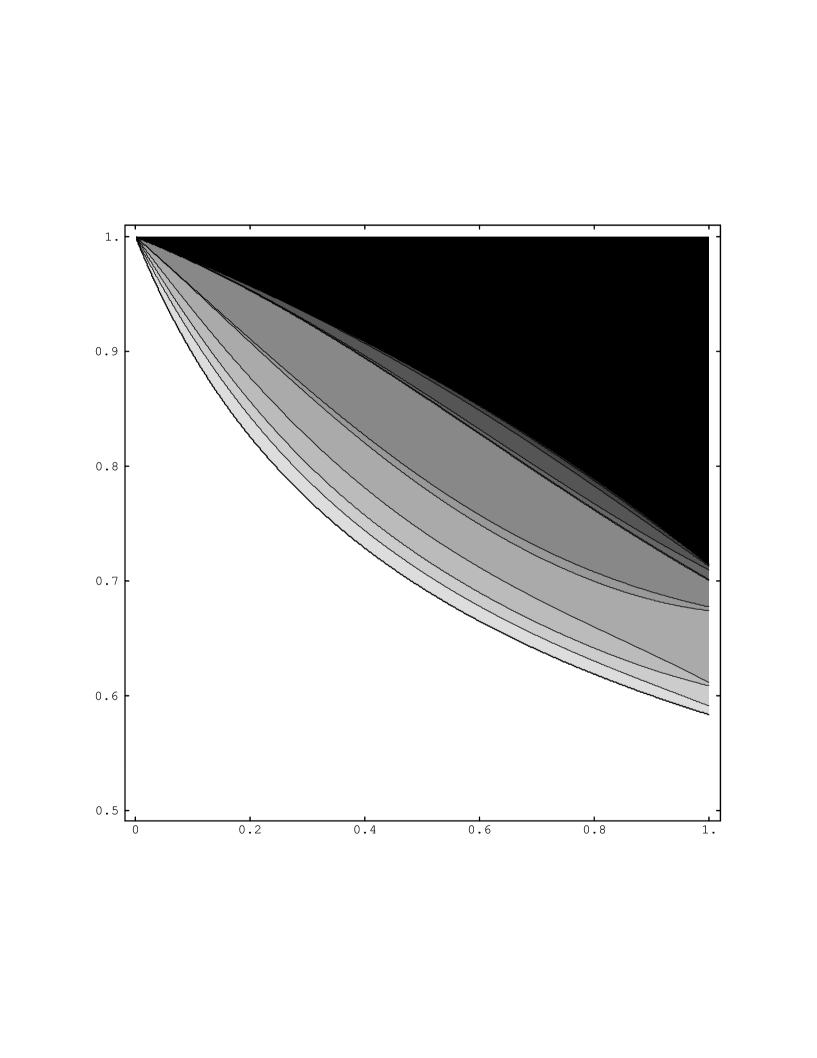
Figure 1: Grey-level plot of the front velocity versus $\epsilon$ (Horizontal axis) and $c$ (Vertical axis) for $a=0.6$ in range 0 (white) to 1 (black). This figure is a projection of a two dimensional Devil’s staircase.

This proof gives also a practical method for computing numerically the front velocity by inverse plotting $\eta$ versus $v$ (see Figure 1). This picture reveals that $\bar{v}(a,1,c)<1$ for some values of $c$. Notice also that for $c\mathchar 13374\relax{1\over 2}$, the velocity is non negative. Moreover, the local map has to be sufficiently non-symmetric, i.e. $c$ must be sufficiently different from ${1\over 2}$, to have travelling fronts. These two comments can be stated from the inequality

$$\eta(a,\epsilon,0)>{1\over 2}.$$

6 The linear stability of fronts with rational velocity

In this section, we improve the linear stability result of the orbits in $\Lambda$ for the fronts and, also for the ghost fronts.

We now consider the configurations $x\in{\cal M}$ for which the code is given by the Heaviside function, namely the kinks. Among the kinks, we shall use the front’s configurations:

$$\left(R_{\sigma}\right)_{s}=\sum_{k=1}^{+\infty}\sum_{n=-k}^{k}l_{n,k}H(s-n+\bar{v}k-\sigma)\quad\forall s\in{{Z}},$$

where $\bar{v}$ is given by (9). Further, let the interval

$${\rm I}_{p\over q}^{0}=\left(\eta({p\over q}^{-}),\eta({p\over q})\right),$$

and $\lceil.\ \rceil$ be the ceiling function. The linear stability of fronts is claimed in the following statement.

Proposition 6.1

For $c\in{\rm I}_{p\over q}^{0}$, let $\delta=\min\left\{c-\eta({p\over q}^{-}),\eta({p\over q})-c\right\}$ and $x$ a kink initial condition such that

$$\exists\sigma\in{{R}}:|\left(R_{\sigma}\right)_{s+\lceil\sigma\rceil}-x_{s+\lceil\sigma\rceil}|\mathchar 13366\relax\delta a^{-k}\quad\forall k\mathchar 13374\relax 0,\quad\forall-2k-1\mathchar 13366\relax s\mathchar 13366\relax 2k,$$ (10)

then $R_{\sigma}^{t}$ and $x^{t}$ have the same code for all times and

$$\lim_{t\rightarrow+\infty}\|R_{\sigma}^{t}-x^{t}\|=0.$$

Remark 6.2

In practice, according to the present phase space, the condition (10) has only to hold for $0\mathchar 13366\relax k\mathchar 13366\relax t_{0}$ where $t_{0}$ is such that $(M+1)a^{t_{0}}<\delta$.

Proof: Since $x$ is a kink that satisfies (10), we have according to the nearest neighbors coupling of the CML:

$$\forall t\mathchar 13374\relax 0\ \left\{\begin{array}[]{ccl}x_{s+\lceil\sigma\rceil}^{t}<c&{\rm if}&s\mathchar 13366\relax-t-1\\ x_{s+\lceil\sigma\rceil}^{t}\mathchar 13374\relax c&{\rm if}&s\mathchar 13374\relax t.\end{array}\right.$$

Using these inequalities, the condition (10) and the definition of $\delta$, one shows by induction, that

$$\forall t\mathchar 13374\relax 0\ |(R_{\sigma}^{t})_{s+\lceil\sigma\rceil}-x_{s+\lceil\sigma\rceil}^{t}|\mathchar 13366\relax\delta a^{-k}\quad\forall k\mathchar 13374\relax 0,\quad\forall-2k-1-t\mathchar 13366\relax s\mathchar 13366\relax 2k+t.$$

The latter induces that both the orbits have the same code for all times. $\Box$

When it exists, let us define the ghost front of velocity ${p\over q}$ by $\{R_{{p\over q}t+\sigma}\}_{t\in{{Z}}}$. For such orbits, the linear stability’s statement is slightly different than for the fronts:

Proposition 6.3

For $c=\eta({p\over q}^{-})$, let $\delta=\phi(-{1\over q})-\phi(-{2\over q})$, and $x$ a kink initial condition such that

$$\exists\sigma\in{{R}}:0<x_{s+\lceil\sigma\rceil}-\left(R_{\sigma}\right)_{s+\lceil\sigma\rceil}\mathchar 13366\relax\delta a^{-k}\quad\forall k\mathchar 13374\relax 0,\quad\forall-2k-1\mathchar 13366\relax s\mathchar 13366\relax 2k,$$

then

$$\lim_{t\rightarrow+\infty}\|R_{{p\over q}t+\sigma}-x^{t}\|=0.$$

The proof is similar to the preceding one noticing that for the ghost front

$$R_{{p\over q}(t+1)+\sigma}={1-a\over a}{\rm L}\theta^{t}+{\rm L}R_{{p\over q}t+\sigma},$$

where $\theta_{s}^{t}=H(s-\lceil{p\over q}t+\sigma\rceil)$ and that $\forall t\mathchar 13374\relax 0$

$$x_{s+\lceil\sigma\rceil}^{t}>(R_{{p\over q}t+\sigma})_{s+\lceil\sigma\rceil}\quad\forall s.$$

7 The interfaces and their velocity

In this section, we study the dynamics and the properties of the code of the orbits for which the state is a kink for all (positive) times.

Definition 7.1

An interface is a positive orbit $\{x^{t}\}_{t\in{{N}}}$ such that

$$\forall t\in{{N}}\ \exists J(x^{t})\in{{Z}}\ :\ \left\{\begin{array}[]{ccl}x_{s}^{t}<c&{\rm if}&s\mathchar 13366\relax J(x^{t})-1\\ x_{s}^{t}\mathchar 13374\relax c&{\rm if}&s\mathchar 13374\relax J(x^{t}),\end{array}\right.$$

where the sequence $\left\{J(x^{t})\right\}_{t\in{{N}}}$ is called the temporal code. The velocity of an interface is the limit

$$v=\lim_{t\rightarrow+\infty}{J(x^{t})\over t},$$

provided it exists.

Notice that the front’s temporal code is given by

$$\lceil\bar{v}t+\sigma\rceil\quad\forall t\in{{Z}},$$ (11)

namely it is uniform [13].

To compare the kinks, the following partial order is considered

Definition 7.2

Let $x,y\in{\cal M}$. We say that $x\prec y$ iff $x_{s}\mathchar 13366\relax y_{s}\quad\forall s\in{{Z}}$.

As a direct consequence of our CML, using this definition, we have

Proposition 7.3

(i) If $x\prec y$ then $F_{\epsilon}x\prec F_{\epsilon}y$.

(ii) If $x\prec y$ are two kinks, then $J(x)\mathchar 13374\relax J(y)$.

Moreover, we can ensure a kink to be the initial condition of an interface in the following ways

Proposition 7.4

Let $x$ be a kink initial condition. If $x_{s}\mathchar 13366\relax x_{s+1}\ \forall s\in{{Z}}$ or, if $\epsilon\mathchar 13366\relax{2\over 3}$, then $\{x^{t}\}_{t\in{{N}}}$ is an interface.

We will also use the asymptotic behaviour in space of the interfaces’ states:

Proposition 7.5

For an interface:

$$\forall t\mathchar 13374\relax 0\ \left\{\begin{array}[]{ccccl}|x_{s}^{t}|&\mathchar 13366\relax&a^{t}M&{\rm if}&s\mathchar 13366\relax J(x^{0})-t-1\\ |1-x_{s}^{t}|&\mathchar 13366\relax&a^{t}M&{\rm if}&s\mathchar 13374\relax J(x^{0})+t.\end{array}\right.$$

This result simply follows from the linearity of the CML and the inequality

$$|J(x^{t})-J(x^{0})|\mathchar 13366\relax t,$$ (12)

which is a consequence of the nearest neighbors’ coupling.

Combining the previous results, one can give some bounds for the temporal code of an interface

Proposition 7.6

If $c\in{\rm I}_{p\over q}^{0}$ and $\{x^{t}\}_{t\mathchar 13374\relax 0}$ is an interface, then

$$\exists\sigma_{1},\sigma_{2}\in{{R}}\ :\ \forall t\mathchar 13374\relax 0\ \lceil{p\over q}t+\sigma_{1}\rceil\mathchar 13366\relax J(x^{t})\mathchar 13366\relax\lceil{p\over q}t+\sigma_{2}\rceil.$$

Proof: We here prove the left inequality, the right one follows similarly. If ${\displaystyle{p\over q}}=-1$, then the statement holds by the inequality (12). Now, let $t_{0}$ be given by Remark 6.2. For ${\displaystyle{p\over q}}\neq-1$ we have

$$\left(R_{0}\right)_{-2t_{0}-1}>0.$$

Let $t_{1}$ be such that $a^{t_{1}}M\mathchar 13366\relax\left(R_{0}\right)_{-2t_{0}-1}$ and let $\tilde{\sigma}_{1}=J(x^{0})-t_{1}-2t_{0}-1$. Define

$$y_{s}=\left\{\begin{array}[]{ccl}x_{s}^{t_{1}}&{\rm if}&s<\tilde{\sigma}_{1}-2t_{0}-1\\ \left(R_{\tilde{\sigma}_{1}}\right)_{s}&{\rm if}&\tilde{\sigma}_{1}-2t_{0}-1\mathchar 13366\relax s\mathchar 13366\relax\tilde{\sigma}_{1}+2t_{0}\\ max\left\{x_{J(x^{t_{1}})}^{t_{1}},x_{s}^{t_{1}}\right\}&{\rm if}&s>\tilde{\sigma}_{1}+2t_{0}.\end{array}\right.$$

Let us check that $x^{t_{1}}\prec y$. For $\tilde{\sigma}_{1}-2t_{0}-1\mathchar 13366\relax s\mathchar 13366\relax\tilde{\sigma}_{1}+2t_{0}$, $y_{s}\mathchar 13374\relax\left(R_{0}\right)_{-2t_{0}-1}\mathchar 13374\relax x_{s}^{t_{1}}$ using the monotony of $R_{\tilde{\sigma}_{1}}$ and the previous proposition.

Hence, by Proposition 7.3, we obtain $J(x^{t+t_{1}})\mathchar 13374\relax J(y^{t})\quad\forall t\mathchar 13374\relax 0$. But $y$ is a kink that satisfies the condition (10) in the framework of Remark 6.2, therefore the left inequality is stated. $\Box$

Finally, the statement on the velocity of any interface, valid for all the values of the parameters, is given by

Theorem 7.7

If $\{x^{t}\}_{t\in{{N}}}$ is an interface then, its velocity exists and

$$\lim_{t\rightarrow+\infty}{J(x^{t})\over t}=\bar{v}(a,\epsilon,c).$$

Proof: For any $\bar{v}$ given by (9), let ${\displaystyle{p_{1}\over q_{1}}}\mathchar 13366\relax\bar{v},\ {\displaystyle{p_{2}\over q_{2}}}\mathchar 13374\relax\bar{v},\ c_{1}\in{\rm I}_{p_{1}\over q_{1}}^{0}$ and $c_{2}\in{\rm I}_{p_{2}\over q_{2}}^{0}$ respectively. If $c\in{\rm I}_{p\over q}^{0}$, then the statement clearly follows from the previous proposition. Moreover, by the monotony of the local map, we have

$$\forall x\in{\cal M}\quad F_{\epsilon,c_{2}}x\prec F_{\epsilon,c}x\prec F_{\epsilon,c_{1}}x,$$

where the dependence on $c$ has been added to the CML. It clearly follows that

$${p_{1}\over q_{1}}\mathchar 13366\relax\liminf_{t\rightarrow+\infty}{J(F_{\epsilon,c}^{t}x)\over t}\mathchar 13366\relax\limsup_{t\rightarrow+\infty}{J(F_{\epsilon,c}^{t}x)\over t}\mathchar 13366\relax{p_{2}\over q_{2}}.$$

The convergence is then ensured by choosing ${\displaystyle{p_{1}\over q_{1}}}$ and ${\displaystyle{p_{2}\over q_{2}}}$ arbitrarily close to $\bar{v}$. $\Box$

To conclude this section, we mention that all these results and, in particular Theorem 7.7, can be extended to the orbits for which the initial condition satisfies

$$\lim_{s\rightarrow\pm\infty}H(x_{s})-H(s)=0.$$

For such orbits, one can prove Theorem 7.7 for the following codes:

$$J_{inf}(x^{t})=\min\{s:x_{s}^{t}\mathchar 13374\relax c\}\quad{\rm and}\quad J_{sup}(x^{t})=\max\{s:x_{s-1}^{t}<c\}.$$

Actually, we have

$$\lim_{t\rightarrow+\infty}{J_{inf}(x^{t})\over t}=\lim_{t\rightarrow+\infty}{J_{sup}(x^{t})\over t}=\bar{v}.$$

8 The nonlinear stability of fronts with rational velocity

An extension of the linear stability result for the fronts can be achieved, also using the CML contracting property which appears in (6), by proving that for all the kink initial conditions, the corresponding interface’s code is identical to a front’s code, at least after a transient.

8.1 The co-existence of fronts and non-uniform fronts

We shall see below that one can only claim the nonlinear stability of fronts in some regions of the parameters. We now justify such restrictions on the latter.

Let, a non-uniform front, be an interface in $\Lambda$ for which the temporal code cannot be written with the relation (11). Using the admissibility condition, one can show the existence of such orbits given a non-uniform code. In this way, we prove in Appendix B, the existence of the non-uniform fronts with velocity ${1\over 2}$ and 0 respectively, when $\epsilon$ is close to 1. Since these orbits are interfaces, they co-exist with the fronts of the same velocity by Theorem 7.7. Moreover, it is possible to state the linear stability of these orbits similarly to Proposition 6.1. Hence, when the non-uniform fronts exist, the fronts do not attract all the kink initial conditions.

8.2 The nonlinear stability for weak coupling

Here, we state the nonlinear stability’s result for the fronts with non negative rational velocity, in the neighborhood of $\epsilon=0$. However, the following assertion can similarly be extended to the fronts with negative velocity.

Let

$$\Delta_{p\over q}\equiv\eta({p\over q})-\eta({p\over q}^{-})=\sum_{k=1}^{+\infty}l_{kp.kq}$$

and, for $\theta\in(0,1)$ let the interval

$${\rm I}_{p\over q}^{\theta}=\left(\eta({p\over q}^{-}),\eta({p\over q})-\theta\Delta_{p\over q}\right),$$

we have:

Theorem 8.1

Given ${p\over q}\in{{Q}}\cap[0,1]$, $a\in(0,1)$ and $\theta\in(0,1)$, there exists $\epsilon_{0}>0$ such that for any kink initial condition $x$:

$$\forall\epsilon\in(0,\epsilon_{0})\quad\forall c\in{\rm I}_{p\over q}^{\theta}\quad\exists\sigma\in{{R}}\ :\ \lim_{t\rightarrow+\infty}\|R_{\sigma}^{t}-x^{t}\|=0.$$

Remark 8.2

For the velocity ${p\over q}=0$, the statement still hold for $\theta=0$.

Moreover for the velocity ${p\over q}=1$, using similar techniques , we have proved that the theorem holds with $\theta=0$ and $\epsilon_{0}=1$ for all the interfaces.

8.3 Proof of the nonlinear stability

In the proof of Theorem 8.1 we assume $\epsilon<{2\over 3}$ then, by Proposition 7.4, all the orbits $\{x^{t}\}_{t\in{{N}}}$ under consideration are interfaces.

In a first place, it is shown that the interfaces propagate forward provided some conditions on the parameters are satisfied.

Proposition 8.3

It exists $\epsilon_{1}>0$ such that for any interface $\{x^{t}\}_{t\in{{N}}}$ and any $c\mathchar 13374\relax{1\over 2}$, we have

$$\forall\epsilon\in(0,\epsilon_{1})\quad\exists t_{0}\ :\ \forall t\mathchar 13374\relax t_{0}\quad J(x^{t+1})\mathchar 13374\relax J(x^{t}).$$

Proof: According to the present phase space, all the orbits of the CML are bounded in the following way:

$$\forall\delta>0\quad\exists t_{0}\ :\ \forall t\mathchar 13374\relax t_{0}\quad-\delta<x_{s}^{t}<1+\delta\quad\forall s\in{{Z}}.$$

In particular, for an interface:

$$x_{J(x^{t})-1}^{t+1}<a(1-{\epsilon\over 2})c+{\epsilon\over 2}+{a\epsilon\delta\over 2}\quad\forall t\mathchar 13374\relax t_{0}.$$

Hence, if $\epsilon$ is sufficiently small, the statement holds for all $c\mathchar 13374\relax{1\over 2}$. $\Box$

Furthermore, we introduce a convenient configuration. Then, after computing the code of the corresponding orbit, we show a dynamical relation between the code of any interface and the code of this particular orbit.

Let

$$\forall j\in{{Z}}\quad\left(S_{j}\right)_{s}={\displaystyle\sum_{k=1}^{+\infty}\sum_{n=-k}^{k}}l_{n,k}H(s-n-j)\quad\forall s\in{{Z}}.$$

Notice that if $c\in(\eta(0^{-}),\eta(0)]$, $S_{j}$ is the front of velocity 0. When $c\not\in(\eta(0^{-}),\eta(0)]$, this configuration is a convenient tool. Actually, the temporal code for the orbit $\{S_{0}^{t}\}_{t\in{{N}}}$ is shown to be given by:

Proposition 8.4

Given ${p\over q}>0$, $a\in(0,1)$ and $\theta\in[0,1)$, there exists $\epsilon_{0}>0$ such that

$$\forall\epsilon\in(0,\epsilon_{0})\quad\forall c\in{\rm I}_{p\over q}^{\theta}\quad J(S_{0}^{t})=\lceil(t+1){p\over q}\rceil\quad\forall t\mathchar 13374\relax 0.$$

Moreover

$$\inf_{s,t}|(S_{0}^{t})_{s}-c|>0.$$

The proof is given in Appendix C.

We now state the main property of an interface’s code.

Proposition 8.5

For an interface we have, under the same conditions of the previous proposition

$$\exists n_{0}\quad\forall n\mathchar 13374\relax n_{0}\quad J(x^{t+n})\mathchar 13366\relax J(S_{0}^{t-1})+J(x^{n})\quad\forall t\mathchar 13374\relax 1.$$ (13)

Proof: Using the relation (6) for $t=n-1$, we obtain the relation between the interfaces’ states and the configuration $S_{j}$:

$$x^{n}=S_{J(x^{n-1})}+{\rm L}\left(x^{n-1}-S_{J(x^{n-1})}\right).$$

By induction, the latter leads to

$$x^{n}=S_{J(x^{n-1})}+{\displaystyle\sum_{k=m+1}^{n-1}}{\rm L}^{n-k}\left(S_{J(x^{k-1})}-S_{J(x^{k})}\right)+{\rm L}^{n-m}\left(x^{m}-S_{J(x^{m})}\right)\quad\forall n>m.$$

Then the monotony of $S_{j}$, the positivity of ${\rm L}$ and Proposition 8.3 induce the following inequality for $m$ large enough and $n>m$

$$\tilde{S}_{n}\prec x^{n},$$

where

$$\tilde{S}_{n}=S_{J(x^{n-1})}+{\rm L}^{n-m}\left(x^{m}-S_{J(x^{m})}\right).$$

Consequently

$$J(x^{t+n})\mathchar 13366\relax J(\tilde{S}_{n}^{t})\quad\forall t\mathchar 13374\relax 0.$$

Now, given $\delta={\displaystyle\inf_{s,t}|(S_{0}^{t})_{s}-c|}$ according to the previous Proposition, let $n_{0}>m$ be such that

$$a^{n_{0}-m}\|x^{m}-S_{J(x^{m})}\|<\delta.$$

It follows that

$$\|\tilde{S}_{n}-S_{J(x^{n-1})}\|<\delta\quad\forall n\mathchar 13374\relax n_{0}+1,$$

and hence, by Proposition 4.1

$$\begin{array}[]{rl}J(\tilde{S}_{n}^{t})=&J(S_{J(x^{n-1})}^{t})\\ =&J(S_{0}^{t})+J(x^{n-1})\quad\forall t\mathchar 13374\relax 0,n\mathchar 13374\relax n_{0}+1.\end{array}$$

$\Box$

Finally, we state the result which ensure a sequence to be uniform.

Lemma 8.6

Let $\{j_{n}\}_{n\in{{N}}}$ be an integer sequence which satisfies the conditions $\forall n\mathchar 13374\relax n_{0}$:

(i) $j_{n+k}\mathchar 13366\relax\lceil{p\over q}k\rceil+j_{n}\quad\quad\forall k\mathchar 13374\relax 0,$

(ii) $j_{n}\mathchar 13374\relax\lceil{p\over q}n+\sigma\rceil\quad$ for a fixed $\sigma\in{{R}}$,

then

$$\exists\gamma\in{{R}}\ {\rm and}\ n_{1}\mathchar 13374\relax n_{0}:\forall n\mathchar 13374\relax n_{1}\quad j_{n}=\lceil{p\over q}n+\gamma\rceil.$$

The proof is given in Appendix D.

Collecting the previous results, we can conclude that, under the conditions of Proposition 8.3 and 8.4, the temporal code of any interface satisfies the condition (i) of Lemma 8.6 (Notice that Proposition 8.3 only serves in the proof of Proposition 8.5). Moreover, this code also satisfies the condition (ii) by Proposition 7.6. Hence, after a transient, all the interfaces have a front’s code. By (6), they consequently converge to a front.

To conclude the proof of Theorem 8.1 in the framework of Remark 8.2, we let $c\in{\rm I}_{0}^{0}$. Hence $J(S_{0}^{t})=0\quad\forall t$. If $c\mathchar 13374\relax{1\over 2}$, the statement holds using Proposition 8.3 and the relation (13). For $c<{1\over 2}$, one can prove the following inequalities:

$$\exists t_{0}\ :\ \forall t\mathchar 13374\relax t_{0}\quad J(x^{t+1})\mathchar 13366\relax J(x^{t}),$$

similarly to Proposition 8.3 and,

$$\exists n_{1}\ :\ \forall n\mathchar 13374\relax n_{1}\quad J(x^{n+1})\mathchar 13374\relax J(S_{0})+J(x^{n}),$$

similarly to the relation (13).

9 Concluding Remarks

In this article, we have considered a simple space-time discrete model for the dynamics of various nonlinear extended systems out of equilibrium. The (piece-wise) linearity of this bistable CML allowed the construction of a bijection between the set of global orbits and the set of admissible codes. When they do not reach the discontinuity, these orbits are linearly stable. For $\epsilon<{1\over 2}$, the CML is injective on ${\cal M}$, then $\Lambda$ can be identified with the limit set

$$\bigcap_{t=0}^{+\infty}F_{\epsilon}^{t}({\cal M}),$$

which attracts all the orbits. These comments justify the study of the global orbits and in particular, the study of fronts which occur widely in extended systems.

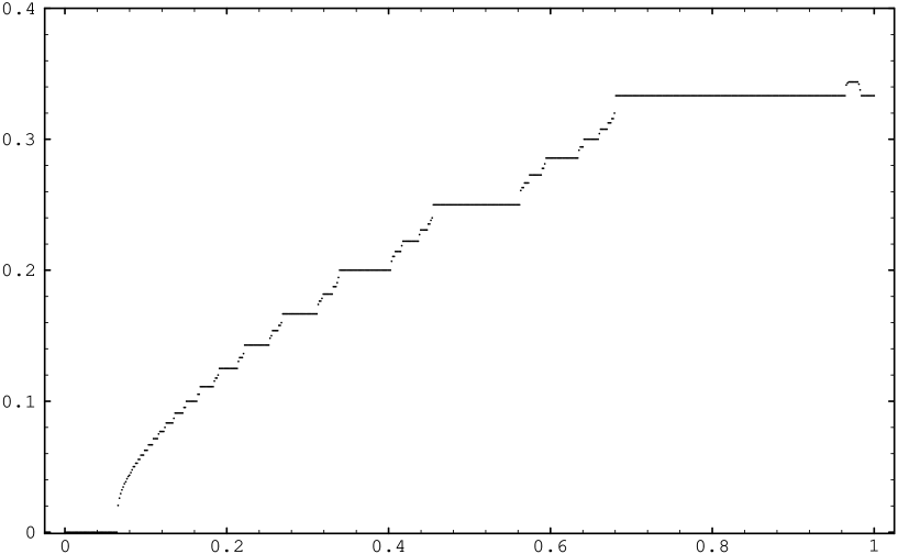
Figure 2: Plot of the front velocity versus $\epsilon$ for $a=0.9$ and $c=0.8216$.

The existence of fronts, with a parametric dependence for their velocity, has been proved using the spatio-temporal coding. The velocity was shown to be increasing with $c$. We have in addition checked numerically that $\bar{v}$ is also an increasing function of $\epsilon$ on $(0,{1\over 2})$ for any $a$ and on $(0,1)$ for any $a\in(0,{1\over 2})$ or for any $a$ if $c$ is such that $\bar{v}(a,1,c)=1$. Moreover, one can find some values of $a$ and $c$ for which the front velocity does not (always) increase with $\epsilon$ (see Figure 2). The spatio-temporal coding also serves to show the existence of other patterns such as non-uniformly propagating interfaces (Appendix B). When these exist, they always co-exist with the fronts of the same velocity.

Furthermore, we have consider the more general dynamics of interfaces. Using the temporal code, we have shown that all these orbits have the front’s velocity uniquely determined by the CML parameters.

The stability of fronts was also proved, firstly with respect to initial conditions close to a front state in their ”center”, and secondly with respect to any kinks for the fronts with non negative rational velocity, assuming some restrictions on the parameters. Actually, the latter allows us to avoid the existence of non-uniform fronts which would attract certain interfaces.

Finally, notice that all the results stated for the orbits that never reach the discontinuity can be extended to some CML’s with a $C^{\infty}$ bistable local map. Actually, one can modify the local map into a $C^{\infty}$ one, in the intervals where the orbits in $\Lambda$ never go, without changing these orbits. In other terms, all our results stated in open sets can be extended to differentiable maps, in particular, the existence and the linear stability of fronts and non-uniform fronts with rational velocity.

These last results show the robustness of fronts in these models. This emphasizes the realistic nature of these models.

Acknowledgments

We want to thank R. Lima, E. Ugalde, S. Vaienti and R. Vilela-Mendes for fruitful discussions and relevant comments. We also acknowledge L. Raymond for his contribution to the nonlinear stability’s proof and, P. Collet for attracting our interest to this piece-wise affine model.

Appendix A Properties of the coefficients $l_{n,k}$

In first place, if $k\mathchar 13374\relax 1$ the following expression holds

$$l_{n,k}=(1-a)a^{k-1}(-1)^{n}\sum_{p=|n|}^{k}\left({-\epsilon\over 2}\right)^{p}{k\choose p}{2p\choose p+n}$$

where ${n\choose p}$ stands for the binomial coefficients. In particular, one has

$$\lim_{\epsilon\rightarrow 0}l_{n,k}=(1-a)a^{k-1}\delta_{n,0},$$

and

$$l_{n,k}=\left\{\begin{array}[]{ccc}{1-a\over a}({a\over 2})^{k}{k\choose{k+n\over 2}}&{\rm if}&{k+n\over 2}\in{{Z}}\\ 0&{\rm if}&{k+n\over 2}\not\in{{Z}}\end{array}\right.\quad{\rm if}\ \epsilon=1.$$

Moreover, one can show that these coefficients have the following generating function

$${1-a\over a}\left({a\epsilon\over 2}+a(1-\epsilon)x+{a\epsilon\over 2}x^{2}\right)^{k}=\sum_{n=0}^{2k}l_{n-k,k}x^{n}\quad\forall x\in{{R}},\ k\mathchar 13374\relax 1.$$

From this function we deduce the relation

$$\sum_{m\in{{Z}}}l_{n-m,t}l_{m,k}={1-a\over a}l_{n,t+k}\quad\forall t,k\mathchar 13374\relax 1.$$

Finally, we prove the following behaviour when $\epsilon$ is small

Proposition A.1

$\forall q\mathchar 13374\relax 1$ and $q\mathchar 13374\relax p\mathchar 13374\relax 0$

(i) ${\displaystyle\lim_{\epsilon\rightarrow 0}}{l_{p,q}\over\epsilon^{p}}>0.$

(ii) ${\displaystyle\lim_{\epsilon\rightarrow 0}{1\over\epsilon^{p}}\sum_{k=q+1}^{+\infty}\sum_{n=p+1}^{k}}l_{n,k}=0.$

Proof: Assume $q\mathchar 13374\relax 1$ and $p\mathchar 13374\relax 0$. (i), From the explicit expression of the $l_{n,k}$, we have

$$\lim_{\epsilon\rightarrow 0}{l_{p,q}\over\epsilon^{p}}={(1-a)a^{q-1}\over 2^{p}}{q\choose p}.$$

Moreover, (ii) is ensured by the relation:

$$\sum_{k=1}^{+\infty}\sum_{n=p+1}^{k}l_{n,k}=\epsilon^{p+1}{a^{p}\over(1-a)^{p+1}}{2^{p}\over\sqrt{1+{2a\epsilon\over 1-a}}}\left({1\over 1+\sqrt{1+{2a\epsilon\over 1-a}}}\right)^{2p+1}.$$

$\Box$

Appendix B The existence of non-uniform fronts

B.1 The non-uniform front with velocity ${1\over 2}$

Consider the following sequence:

$$j_{t}=\lfloor{t\over 4}\rfloor+\lfloor{t+1\over 4}\rfloor\quad\forall t\in{{Z}},$$

and

$$z_{s}^{t}=\sum_{k=1}^{+\infty}\sum_{n=-k}^{k}l_{n,k}H(s-n-j_{t-k})\quad\forall s,t\in{{Z}}$$

the corresponding orbit in $\Lambda$, namely a non-uniform front with velocity ${1\over 2}$. Actually, $j_{t+4}=j_{t}+2$ but it does not correspond to the temporal code of the front of velocity ${1\over 2}$. The existence of this particular orbit is stated in

Proposition B.1

$\exists\tilde{\epsilon}>0$ such that $\forall\epsilon\in(\tilde{\epsilon},1]$, there exists an interval $\tilde{\rm I}$ so that

$$\forall c\in\tilde{\rm I}\quad\forall t\in{{Z}}\quad F_{\epsilon}(z^{t})=z^{t+1}.$$

Proof: $z_{s}^{t}$ is monotone in $s$. Then one has to prove that, in a neighborhood of $\epsilon=1$,

$$\min_{t}z_{j_{t}}^{t}>\max_{t}z_{j_{t}-1}^{t},$$

in order for the statement to hold for $\tilde{\rm I}=\left({\displaystyle\max_{t}}z_{j_{t}-1}^{t},{\displaystyle\min_{t}}z_{j_{t}}^{t}\right]$.

Let $\Delta_{k}^{t}=j_{t}-j_{t-k}$. We have

$$\Delta_{k}^{t+4}=\Delta_{k}^{t}\quad{\rm and}\quad\Delta_{k+4}^{t}=\Delta_{k}^{t}+2,$$

and

$$\min_{t}\Delta_{k}^{t}=\Delta_{k}^{2}\quad{\rm and}\quad\max_{t}\Delta_{k}^{t}=\Delta_{k}^{0}.$$

Using these properties, we show that

$$\min_{t}z_{j_{t}}^{t}-\max_{t}z_{j_{t}-1}^{t}=\sum_{k=1}^{+\infty}(-1)^{k}l_{k,2k}.$$

From the expression of the $l_{k,2k}$ for $\epsilon=1$, it follows that

$$\lim_{\epsilon\rightarrow 1^{-}}(\min_{t}z_{j_{t}}^{t}-\max_{t}z_{j_{t}-1}^{t})>0.$$

$\Box$

Notice that (when it exists) this non-uniform front lies between the fronts of code $\lfloor{t-1\over 2}\rfloor$and $\lfloor{t\over 2}\rfloor$.

B.2 The oscillating front

Here, we consider a non-uniform front of velocity 0. In particular, the one for which the temporal code writes:

$$J_{t}={1+(-1)^{t}\over 2}\quad\forall t\in{{Z}}.$$

Naturally, the expression for this orbit can be written similarly to the previous one but now, with this code’s relation. Let $\{Z^{t}\}_{t\in{{Z}}}$ denotes the orbit. Its existence is claimed in

Proposition B.2

$\exists\check{\epsilon}>0$ such that $\forall\epsilon\in(\check{\epsilon},1]$, there exists an interval $\check{\rm I}$ so that

$$\forall c\in\check{\rm I}\quad\forall t\in{{Z}}\quad F_{\epsilon}(Z^{t})=Z^{t+1}.$$

Similarly to the previous proof, the existence of this orbit is ensured by the relation

$$\min_{t}Z_{J_{t}}^{t}-\max_{t}Z_{J_{t}-1}^{t}=\sum_{k=1}^{+\infty}(-1)^{k}l_{0,k}.$$

Furthermore, using these technique, we can prove the existence of another non-uniform fronts. All these orbits exist only in a neighborhood of $\epsilon=1$, they disappear for $\epsilon$ close to 0.

Appendix C Proof of Proposition 8.4

Since the fronts’ configurations are increasing functions in space, the following ordering holds:

$$S_{0}\prec R_{p\over q}.$$

Hence, using Proposition 7.3, we obtain for $c\in{\rm I}_{p\over q}^{\theta}$:

$$\left(S_{0}^{t}\right)_{\lceil{p\over q}(t+1)\rceil-1}\mathchar 13366\relax\left(R_{{p\over q}(t+1)}\right)_{\lceil{p\over q}(t+1)\rceil-1}<c\quad\forall t\mathchar 13374\relax 0.$$

To prove the statement, we then show by induction that

$$\left(S_{0}^{t}\right)_{\lceil{p\over q}(t+1)\rceil}>c\quad\forall t\mathchar 13374\relax 0,$$

in a neighborhood of $\epsilon=0$.

Using the relations (2) and (A1) to write

$$\left(S_{0}^{t}\right)_{s}=\sum_{k=1}^{t}\sum_{n=-k}^{k}l_{n,k}H(s-n-J(S_{0}^{t-k}))+\sum_{k=t+1}^{+\infty}\sum_{n=-k}^{k}l_{n,k}H(s-n),$$

we consider the following decomposition

$$\left(S_{0}^{t}\right)_{\lceil{p\over q}(t+1)\rceil}-\eta({p\over q})+\theta\Delta_{p\over q}=P_{1}+P_{2}+P_{3}+P_{4},$$

where

$$\begin{array}[]{rcl}P_{1}&=&{\displaystyle\sum_{k=1}^{t}\sum_{n=-k}^{k}}l_{n,k}\left(H(\lceil{p\over q}(t+1)\rceil-\lceil{p\over q}(t-k+1)\rceil-n)-H({p\over q}k-n)\right)\\ P_{2}&=&{\displaystyle\sum_{n=-t-1}^{t+1}}l_{n,t+1}\left(H(\lceil{p\over q}(t+1)\rceil-n)-H({p\over q}(t+1)-n)\right)\\ P_{3}&=&{\displaystyle\sum_{k=t+2}^{+\infty}\sum_{n=-k}^{k}}l_{n,k}\left(H(\lceil{p\over q}(t+1)\rceil-n)-H({p\over q}k-n)\right)\\ P_{4}&=&\theta{\displaystyle\sum_{k=1}^{+\infty}}l_{kp,kq}.\end{array}$$

We have the following inequalities:

$\begin{array}[]{ccl}P_{1}&\mathchar 13374\relax&0\quad{\rm since}\quad\lceil{p\over q}(t+1)\rceil-\lceil{p\over q}(t-k+1)\rceil\mathchar 13374\relax\lfloor{p\over q}k\rfloor\ \forall k,t\in{{N}}.\\ P_{2}&\mathchar 13374\relax&0\quad{\rm and}\quad P_{2}=l_{\lceil{p\over q}(t+1)\rceil,t+1}\quad{\rm if}\quad t<q-1.\\ P_{3}&\mathchar 13374\relax&{\displaystyle\sum_{k=t+2}^{+\infty}\sum_{n=-k}^{k}}l_{n,k}\left(H(\lceil{p\over q}(t+1)\rceil-n)-H(k-n)\right)\\ &\mathchar 13374\relax&-{\displaystyle\sum_{k=t+2}^{+\infty}\sum_{n=\lceil{p\over q}(t+1)\rceil+1}^{k}}l_{n,k}.\\ P_{4}&\mathchar 13374\relax&\theta l_{p,q}.\end{array}$

Then one can write, for $0\mathchar 13366\relax t<q-1$:

$$P_{1}+P_{2}+P_{3}+P_{4}\mathchar 13374\relax l_{\lceil{p\over q}(t+1)\rceil,t+1}-\sum_{k=t+2}^{+\infty}\sum_{n=\lceil{p\over q}(t+1)\rceil+1}^{k}l_{n,k},$$

and for $t\mathchar 13374\relax q-1$:

$$P_{1}+P_{2}+P_{3}+P_{4}\mathchar 13374\relax\theta l_{p,q}-\sum_{k=q+1}^{+\infty}\sum_{n=p+1}^{k}l_{n,k}.$$

Hence using Proposition A.1, in both cases $P_{1}+P_{2}+P_{3}+P_{4}>0$ if $\epsilon$ is sufficiently small. $\Box$

Appendix D Proof of Lemma 8.6

By (ii), it exists $n_{1}\mathchar 13374\relax n_{0}$ such that

$$j_{n_{1}}-n_{1}{p\over q}\mathchar 13366\relax j_{n}-n{p\over q}\quad\forall n\mathchar 13374\relax n_{1}.$$

Then, also using (i), one has

$$0\mathchar 13366\relax j_{n_{1}+t}-j_{n_{1}}-t{p\over q}\mathchar 13366\relax\lceil t{p\over q}\rceil-t{p\over q}<1\quad\forall t\mathchar 13374\relax 0,$$

which implies that

$$\lfloor j_{n_{1}+t}-j_{n_{1}}-t{p\over q}\rfloor=0\quad\forall t\mathchar 13374\relax 0.$$

Now it is straightforward to see that

$$j_{n}=\lceil n{p\over q}+\gamma\rceil\quad\forall n\mathchar 13374\relax n_{1},$$

where $\gamma=j_{n_{1}}-n_{1}{p\over q}.\Box$

References

- [1] M.C. Cross and P.C. Hohenberg, “Pattern formation outside equilibrium”, Rev. Mod. Phys., 65, 1993, 851-1113.
- [2] K. Showalter, “Quadratic and cubic reaction-diffusion fronts”, Nonlinear Science Today 4(4), 1995.
- [3] H. Levine and W.R. Reynolds, “CML techniques for simulating interfacial phenomena in reaction-diffusion systems”, Chaos 2(3), 1992, 337-342.
- [4] J. Elkinani and J. Villain, “Growth roughness and instabilities due to the Schwoebel effect: a one-dimensional model”, J. Phys. (France) 4 (1994) 949-973.
- [5] P. Collet and J.P. Eckmann, “Instabilities and fronts in extended systems”, Princeton University Press, Princeton, NJ, 1990.
- [6] A-D. Defontaines, Y. Pomeau and B. Rostand, “Chain of coupled bistable oscillators: a model”, Physica D, 46 (1990) 210-216.
- [7] J.P. Keener “Propagation and its failure in coupled systems of discrete excitable cells”, SIAM J. Appl. Math. 47 (1987), 556-572.
- [8] V.S. Afraimovich and V.I. Nekorkin, “Chaos of traveling waves in a discrete chain of diffusively coupled maps”, Int. J. Bif. Chaos 4 (1994), 631-637.
- [9] R. Carretero-González, D.K. Arrowsmith and F. Vivaldi. “Mode-locking in CML”, Submitted to Physica D.
- [10] K. Kaneko, editor, “Theory and applications of Coupled Map Lattices”, Wiley, New-York, 1993.
- [11] S. Aubry, D. Escande, J.P. Gaspard, P. Manneville and J. Villain. “Structures et instabilités”. Les éditions de physique, Orsay, 1986.
- [12] B. Fernandez, “Existence and stability of steady fronts in bistable CML”. J. Stat. Phys., 82 (3), 1996, 931-950.
- [13] B. Fernandez and L. Raymond, “The propagating fronts in bistable CML”, J. Stat. Phys. (to be published)
- [14] N. Bird and F. Vivaldi, “Periodic orbits of the sawtooth maps”, Physica D 30, (1988) 164-176.
- [15] R. Coutinho, “Discontinuous rotations”, (Preprint).
- [16] R. Coutinho and B. Fernandez, “The phenomenology of bistable CML”, (in preparation).