Structure of Complex-Periodic and Chaotic Media with Spiral Waves

Abstract

The spatiotemporal structure of reactive media supporting a solitary spiral wave is studied for systems where the local reaction law exhibits a period-doubling cascade to chaos. This structure is considerably more complex than that of simple period-1 oscillatory media. As one moves from the core of the spiral wave the local dynamics takes the form of perturbed, period-doubled orbits whose character varies with spatial location relative to the core. An important feature of these media is the existence of a curve where the local dynamics is effectively period-1. This curve arises as a consequence of the necessity to reconcile the conflict between the global topological organization of the medium induced by the presence of a spiral wave and the topological phase space structure of local orbits determined by the reaction rate law. Due to their general topological nature, the phenomena described here should be observable in a broad class of systems with complex periodic behavior.

I Introduction

Spiral waves are spatio-temporal patterns typically found in distributed media with active elements. They have been studied extensively for excitable and oscillatory media. [1, 2] For both types of media, it is conventional to consider systems with two dynamical variables. Activator-inhibitor or propagator-controller systems are often used to analyse spiral dynamics in excitable media [2, 3], while the complex Ginzburg–Landau equation is the prototypical model describing spatially-distributed oscillatory media near the Hopf bifurcation point [4].

Spiral waves may also exist in media where the local dynamics supports complex periodic or even chaotic motion that cannot be represented in a two-dimensional phase plane. Various patterns involving rotating spiral waves have been observed in coupled map lattices or reaction-diffusion dynamics based on the Rössler chaotic attractor [5]. The three-variable reaction-diffusion system with chaotic local reaction kinetics given by the Willamowski-Rössler rate law [6] has been studied in [7]. Stable spiral waves exist in this system and the nucleation and annihilation of spiral pairs leading to spiral turbulence have been observed. The change of dimensionality of phase space from two to three significantly complicates the description of the dynamics. Descriptions in terms of phase and amplitude, well established for two-variable models, cannot be directly generalized. Although several definitions have been proposed for the phase of chaotic oscillations, all of them suffer from some degree of ambiguity (see [8] for a discussion). Similar difficulties arise in the consideration of nonchaotic oscillatory dynamics which is nevertheless more complex than a single loop in phase space; for example, in the oscillations that appear in the period doubling cascade to chaos or in the mixed-mode oscillations observed in experiments in chemical systems. [9]

In this paper we study the spatiotemporal organization of a reacting medium which supports a single spiral wave and where the local rate law exhibits period-$2^{n}$ or chaotic oscillations. Through an analysis of the dynamics at different spatial points in the medium we show that a number of phenomena arise for $n>0$ which are nonexistent in period-1 oscillatory media. Section II introduces the model and presents some features of the spiral wave behavior in a chaotic medium. The local dynamics in the medium is considered in detail in Sec. III. The analysis allows one to identify the loop exchange process for local trajectories and the complicated pattern of the distribution of different types of local dynamics in the medium. A characteristic feature of this distribution is the existence of a curve where the local dynamics is effectively period-1. Section IV introduces a coarse-grained description of $2^{n}$-periodic local orbits which allows one to characterize the local dynamics that is observed in the medium. The topological conflict between the phase space structure of local trajectories and the constraints imposed on the medium by the existence of a spiral wave is considered in Sec. V. We show that the observed changes of the local orbits are necessary to maintain the global coherence of the medium. The conclusions of the study are presented in Sec. VI.

II Spiral Waves in Periodic and Chaotic Media

While many aspects of the phenomena we describe in this paper are general and apply to systems in which complex periodic or chaotic orbits exit, we consider situations where a chaotic attractor arises by a period-doubling cascade and confine our simulations to the Willamowski-Rössler (WR) model [6],

$$A_{1}+X \mathrel{\mathop{\kern 0.0pt{\rightleftharpoons}}\limits^{{k_{1}}}_{k_{-1}}} 2X,\;\;X+Y\mathrel{\mathop{\kern 0.0pt{\rightleftharpoons}}\limits^{{k_{2}}}_{k_{-2}}}2Y,$$ (1)

$$A_{5}+Y \mathrel{\mathop{\kern 0.0pt{\rightleftharpoons}}\limits^{{k_{3}}}_{k_{-3}}} A_{2},\;\;X+Z\mathrel{\mathop{\kern 0.0pt{\rightleftharpoons}}\limits^{{k_{4}}}_{k_{-4}}}A_{3},$$ (2)

$$A_{4}+Z \mathrel{\mathop{\kern 0.0pt{\rightleftharpoons}}\limits^{{k_{5}}}_{k_{-5}}} 2Z\;.$$ (3)

Only the $X$, $Y$ and $Z$ species vary with time; all others are assumed fixed by flows of reagents. Study of this model allows us to illustrate most features of the structure of a spatially distributed medium supporting spiral waves. In addition, it is useful to deal with a specific example since certain aspects of the analysis of periodic and chaotic orbits in high-dimensional concentration phase spaces rely on geometrical constructions that pertain to a specific class of attractors.

The rate law that follows from the mechanism (2) is

$${dc_{x}(t)\over dt} = \kappa_{1}c_{x}-\kappa_{-1}c_{x}^{2}-\kappa_{2}c_{x}c_{y}+\kappa_{-2}c_{y}^{2}-\kappa_{4}c_{x}c_{z}$$ (5)

$$+\kappa_{-4}=R_{x}({\bf c}(t))\;,$$

$${dc_{y}(t)\over dt} = \kappa_{2}c_{x}c_{y}-\kappa_{-2}c_{y}^{2}-\kappa_{3}c_{y}+\kappa_{-3}$$ (7)

$$=R_{y}({\bf c}(t))\;,$$

$${dc_{z}(t)\over dt} = -\kappa_{4}c_{x}c_{z}+\kappa_{-4}+\kappa_{5}c_{z}-\kappa_{-5}c_{z}^{2}=R_{y}({\bf c}(t))\;,$$ (8)

where the rate coefficients $\kappa_{i}$ include the concentrations of any species held fixed by constraints. We take $\kappa_{2}$ to be the bifurcation parameter while all other coefficients are fixed: ($\kappa_{1}=31.2,\kappa_{-1}=0.2,\kappa_{-2}=0.1,\kappa_{3}=10.8,\kappa_{-3}=0.12,\kappa_{4}=1.02,\kappa_{-4}=0.01,\kappa_{5}=16.5,\kappa_{-5}=0.5$). In this parameter region the WR model has been shown [10] to possess a chaotic attractor arising from a period-doubling cascade as $\kappa_{2}$ is varied in the interval [1.251,1.699].

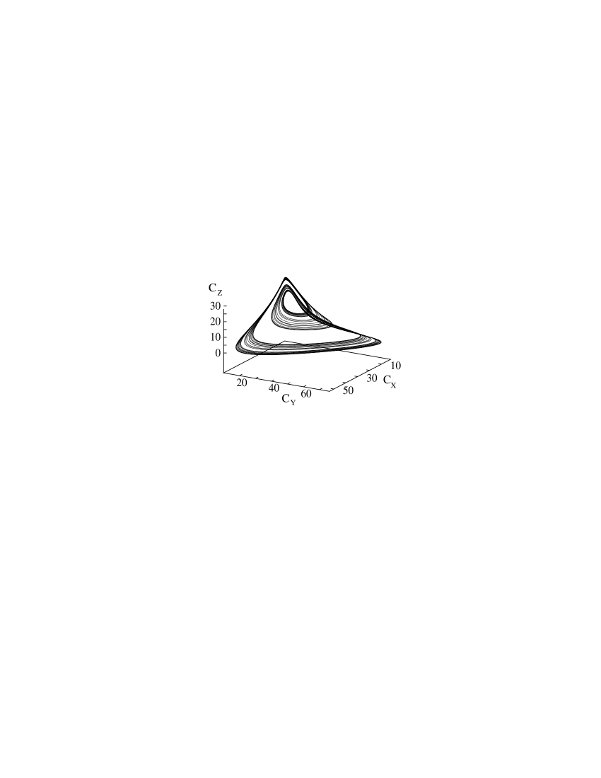
FIG. 1.: Chaotic attractor for the Willamowski-Rössler model at $\kappa_{2}=1.567$.

Figure 1 shows the four-banded chaotic attractor at $\kappa_{2}=1.567$. Throughout the entire parameter domain $\kappa_{2}\in[1.251,1.699]$ the system’s attractor is oriented so that its projection onto the $(c_{x},c_{y})$ plane exhibits a folded phase space flow circulating around the unstable focus ${\bf c^{*}}$. This allows one to introduce a coordinate system in the Cartesian $(c_{x},c_{y},c_{z})$ phase space which is appropriate for the description of the attractor. We take the origin of a cylindrical coordinate system $(\rho,\phi,z)$ at ${\bf c^{*}}$ so that the $z$ and zero-phase-angle ($\phi=0$) axes are directed along the $c_{z}$ and $c_{y}$ axes, respectively. The phase angle $\phi$ increases along the direction of flow as shown in Fig. 2.

FIG. 2.: Cylindrical coordinate frame $(\rho,\phi,z)$ with origin at ${\bf c}^{*}$ in the $(c_{x},c_{y},c_{z})$ phase space. A period-2 orbit is shown in this coordinate frame.

For a period-1 oscillation $\phi$ coincides with the usual definition of the phase and uniquely parametrizes the attractor $\rho_{a}=\rho_{a}(\phi),z_{a}=z_{a}(\phi),\phi\in[0,2\pi)$. After the first period-doubling this parametrization is no longer unique since the periodic orbit does not close on itself after $\phi$ changes by $2\pi$. For a period-$2^{n}$ orbit $2^{n}$ of its points lie in any semi-plane $\phi=\phi_{0}$. The angle variable $\Phi\in[0,2^{n}\cdot 2\pi)$ may be used to parametrize the period-$2^{n}$ attractor if one acknowledges that all $\Phi$ from the interval $[0,2^{n}\cdot 2\pi)$ are different but any two values of $\Phi$, $\Phi_{1}$ and $\Phi_{2}$, with $\Phi_{2}=\Phi_{1}+2^{n}\cdot 2\pi$, are equivalent. For a chaotic orbit $(n\rightarrow\infty)$ all angles $\Phi\in[0,\infty)$ are non-degenerate. When $\Phi$ is defined in this way it is no longer an observable. Indeed, any $\Phi\in[0,2^{n}\cdot 2\pi)$ can be represented as $\Phi=\phi+m\cdot 2\pi$ where $\phi\in[0,2\pi)$ and $m\in{\bf N}$. While $\phi$ is just the angle coordinate in the $(\rho,\phi,z)$ system and is a single-valued function of the instantaneous concentrations $\phi=\phi(c_{x}(t),c_{y}(t),c_{z}(t))$, the integer number of turns $m$ can be calculated only if the entire attractor is known.

The spatially-distributed system is described by the reaction-diffusion equation,

$${\partial{\bf c}({\bf x},t)\over\partial t}={\bf R}({\bf c}({\bf x},t))+D\nabla^{2}{\bf c}({\bf x},t)\;,$$ (9)

where we have assumed the diffusion coefficients of all species are equal. If the rate law parameters correspond to a period-1 limit cycle, we may initiate a spiral wave in the medium and describe its dynamics and structure using well-developed methods. The core of such a spiral wave is a topological defect which is characterized by the topological charge [11]

$${1\over 2\pi}\oint\nabla\phi({\bf r})\cdot d{\bf l}=n_{t}\;,$$ (10)

where $\phi({\bf r})$ is the local phase and the integral is taken along a closed curve surrounding the defect. To obtain additional insight into the organization of the medium around the defect the local dynamics may be considered. For this purpose we introduce a polar coordinate system ${\bf r}={\bf x}-{\bf r}_{d}(t)=(r,\theta)$ centered at the defect whose (possibly time-dependent position) is ${\bf r}_{d}(t)$. Let ${\bf c}({\bf r},t)$ be a vector of local concentrations at space point ${\bf r}=(r,\theta)$. A local trajectory in the concentration phase space from $t=t_{0}$ to $t=t_{0}+\tau$ at point ${\bf r}$ in the medium will be denoted by

$$C({\bf r}|t_{0},\tau)=\{{\bf c}({\bf r},t)|t\in[t_{0},t_{0}+\tau]\}\;.$$ (11)

Figure 3 shows a number of local trajectories $C(r,\theta|t_{0},\tau)$ at points with increasing separation $r$ from the defect for a period-1 oscillation at $\kappa_{2}=1.420$. One sees that as $r\rightarrow 0$ the oscillation amplitude decreases and the limit cycle shrinks to the phase space point ${\bf c}^{*}_{d}$ corresponding to the spiral core. The results of our simulations show that the value of ${\bf c}^{*}_{d}$ differs only slightly from ${\bf c^{*}}$ which is chosen as the origin of the coordinate frame $(\rho,\phi,z)$. Thus, the angle $\phi$ can serve as a phase that characterizes all points in the period-1 oscillatory medium except for a small neighborhood of the defect with radius $r\approx 1$. [12] The concentration field ${\bf c}({\bf r},t)$ is organized so that the instantaneous $(c_{x},c_{y},c_{z})$ phase space representation of the local concentration on any closed path in the medium surrounding the defect is a simple closed curve encircling ${\bf c^{*}}$. For large $r$, $r\geq r_{max}$ (in Fig. 3 $r_{max}\approx 40$), one finds that $C(r,\theta|t_{0},\tau)$ ceases to change shape and is indistinguishable from the period-1 attractor of (5) on the scale of the figure.

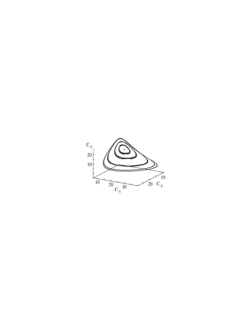
FIG. 3.: Local trajectories calculated for the period-1 oscillatory medium ($\kappa_{2}=1.420$) at radii 5, 10, 20, 30, 40, 56, and fixed $\theta$. The periodic orbits grow monotonically in size with $r$; the difference between trajectories corresponding to $r=40$ and $r=56$ is not resolved on the scale of the figure. Local orbits appear to be independent on angle $\theta$. The location of ${\bf c}^{*}$ is designated by a diamond.

One may initiate the analog of a defect in $2^{n}$-periodic and chaotic media. The defect serves as the core of a spiral wave which may exist even if the oscillation is not simply period-1. A defect was introduced in the center of the medium by fixing $c_{z}({\bf r})=c^{*}_{z}$ and choosing initial concentrations $(c_{x}({\bf r}),c_{y}({\bf r}))$ to produce orthogonal spatial gradients. The influence of the symmetry of the spatial domain on the dynamics was investigated by performing simulations on square $(L\times L)$ arrays as well as on disk-shaped domains with radius $R$. No-flux boundary conditions were used to prevent the formation of defects with opposite topological charge within the medium and to minimize effects arising from the self-interaction of spiral waves. The implementation of these initial and boundary conditions does not guarantee the formation of a solitary stable spiral wave; new spiral pairs and other patterns (e.g. pacemakers) may appear as a result of instabilities of the spiral arm and lead to spiral turbulence. The ability to maintain a stationary spiral wave in the center of the medium is sensitive to the parameters. For various values of the system size and rate constants the defect can move along expanding or contracting spiral trajectories or trajectories with complex “daisy”-like forms [13]. Simulations show that the stability of a spiral wave with a stationary core located at the center of the medium increases with the system size and for rate constants lying close to the chaotic regime within the period-doubling cascade. In the following we restrict our considerations to parameters that lead to the formation of a single spiral wave whose core is stationary and lies in the center of the domain. Long transient times ($\approx 10^{2}$ spiral revolutions) are often necessary to reach this attracting state.

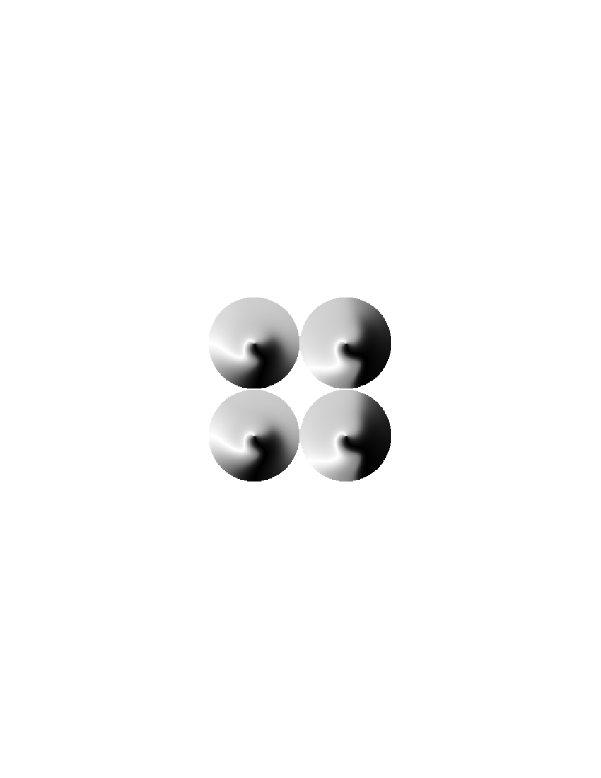
FIG. 4.: Frames showing a rotating spiral wave in the chaotic ($\kappa_{2}=1.567$) disk-shaped medium with $R=80$. The local angle variable $\phi(r,\theta,t)$ is shown as grey shades. Time increases from left to right and from top to bottom. The frames are separated by one period of spiral revolution $T_{r}$. The integration time step is $\Delta t=10^{-4}$ and the scaled diffusion coefficient is $D\Delta t/(\Delta x)^{2}=10^{-2}$.

Figure 4 shows four consecutive states of the disk-shaped medium with $R=80$, separated by one period of the spiral rotation, $T_{r}$, for $\kappa_{2}=1.567$ where the rate law supports a chaotic attractor. Only within a sufficiently small region with radius $r\approx 20$ centered on the defect does the medium return to the same state after one period of spiral rotation. At points farther from the defect the system appears to return to the same state only after two spiral rotation periods. The transition from period-1 to period-2 behavior occurs smoothly along any ray emanating from the defect.

III Analysis of Local Dynamics

More detailed information may be obtained from an investigation of the local dynamics of the medium supporting a spiral wave. Local trajectories $C({\bf r}|t_{0},\tau)$ were computed along rays emanating from the defect at various angles $\theta$. Figure 5 (left column) shows short-time trajectories ($\tau\approx 10T_{r}$) at different radii $r$ and arbitrary but large $t_{0}$. These trajectories clearly demonstrate that the local dynamics undergoes transformation from small-amplitude period-1 oscillations in the neighborhood of the defect to period-4 oscillations near the boundary.[14]

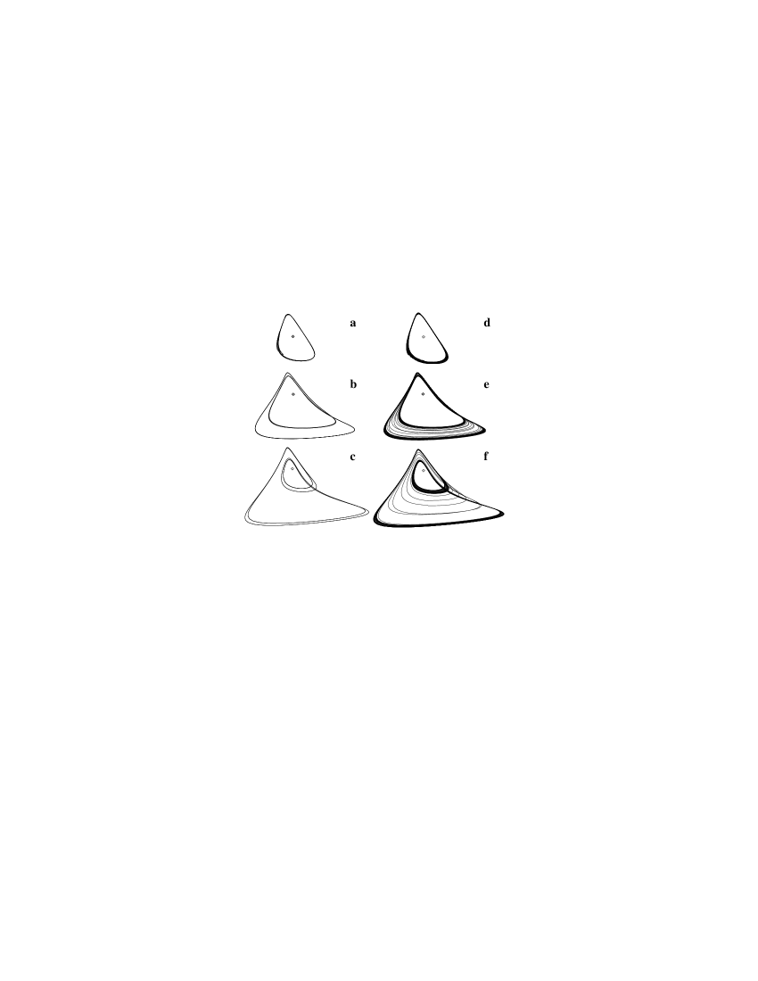
FIG. 5.: Local trajectories $C(r|\,t_{0},\tau)$ for the disk-shaped medium ($\kappa_{2}=1.567,\;R=80$): (a, d) $r=10$; (b, e) $r=35$; (c, f) $r=76$. The observation times are $\tau\approx 10T_{r}$ for left column and $\tau=80T_{r}$ for right column. All the trajectories are shown on the same scale.

The well-resolved period-doubling structure of $C({\bf r}|t_{0},\tau)$ is destroyed if the time of observation $\tau$ becomes sufficiently large. The right column of Fig. 5 shows trajectories sampled at the same spatial locations but with the time of observation $\tau=80T_{r}$. These long-time trajectories appear to be “noisy” period-1 and period-2 orbits: the trajectory in panel (d) is a thickened period-1 orbit while both the period-2 (panel (b)) and period-4 (panel (c)) orbits now appear as thickened period-2 orbits in panels (e) and (f) with trajectory segments lying between the period-2 bands. As $\tau$ tends to infinity the resulting local attractor, $C(r)$, is independent of $t_{0}$ and the angle $\theta$.

A First-return maps

An analysis of the local trajectories shows that the period-doubling phenomenon is not a monotonic function of $r$. Consider the first return map constructed from a Poincaré section of a local trajectory $C({\bf r}|t_{0},\tau)$ in the following way: choose the plane $c_{y}=c_{y}^{*}$ with normal ${\bf n}$ along the $c_{y}$ axis as the surface of section and select those intersection points where ${\bf n}$ forms a positive angle with the flow. This yields a set $\{(c_{x}({\bf r},t_{n}),c_{z}({\bf r},t_{n}))|n\in[1,N]\}$ where $t_{0}<t_{1}<t_{2}<\ldots<t_{N}<t_{0}+\tau$ is a sequence of times at which the trajectory crosses the surface of section. For the WR model the points $(c_{x}({\bf r},t_{n}),c_{z}({\bf r},t_{n}))$ lie on a curve which deviates only slightly from a straight line. Consequently, we may choose either $c_{x}$ or $c_{z}$ to construct the first return map. Let $\xi_{n}({\bf r})=c_{x}({\bf r},t_{n})$ denote a point in the Poincaré section. The relation $\xi_{n+1}({\bf r})=f(\xi_{n}({\bf r}))$ between the successive intersections of the Poincaré surface defines the local first return map,

$$g({\bf r}|t_{0},\tau) = \{(\xi_{n}({\bf r}),\xi_{n+1}({\bf r}))$$ (13)

$$|\,t_{n}\in[t_{0},t_{0}+\tau],n\in[1,N]\}\;.$$

Combining such maps for all $r$ along some ray emanating from the defect at an angle $\theta$, we obtain the cumulative first return map,

$$G(\theta|t_{0},\tau)=\bigcup_{r\in(0,R)}g(r,\theta|t_{0},\tau)\;.$$ (14)

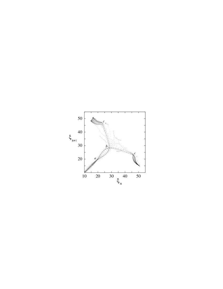
FIG. 6.: Cumulative first return map $G$ constructed for the disk-shaped array ($\kappa_{2}=1.567,\;R=80$). The letters indicate the $r$ values discussed in the text: (a) 20, (b) 31 and (c) 43.

For sufficiently long times $\tau$, $g$ is independent of $\theta$ and $t_{0}$. Letting $\lim_{\tau\to\infty}g(r,\theta|t_{0},\tau)=g(r)$, we may write the corresponding cumulative first return map as $G=\lim_{\tau\to\infty}G(\theta|t_{0},\tau)$. Figure 6 shows $G$ for the disk-shaped medium under consideration. The first return map is comprised of several branches which can be identified as thread-like maxima of the first return map point density. These branches are parametrized by the spatial coordinate with $r$ increasing from the bottom left corner to the ends of the wide-spread arms of $G$ (cf. Fig. 6). Generally for $r\leq 40$ points lying on lines $\xi_{n}(r)+\xi_{n+1}(r)={\rm const}$ belong to the same $g(r)$ though overlaps of neighboring $g$-map points are common. Thus, measuring the separation between branches of $G$ in the direction perpendicular to the bisectrix one can determine the character of $C(r)$. In spite of some evidence of fine structure, from the fact that map points are located along the bisectrix in Fig. 6 one can infer that up to $r=20$ the local dynamics is predominantly period-1. Starting from $r=21$ (labeled by $a$ in Fig. 6), $G$ splits into two branches which diverge from the bisectrix indicating a period-2 structure of $C(r)$. As $r$ increases these branches bend and cross the bisectrix at $r=31$ (labeled by $b$ in Fig. 6), indicating a return of the local dynamics to the period-1-like pattern. After this crossing the separation between the branches grows rapidly reflecting the development of period-2 structure. An examination of the main branches of $G$ reveals period-4 fine structure. This period-4 structure is visible for $r>28$ and beyond $r\approx 43$ (labeled by $c$ in Fig. 6) it becomes prominent and can be easily seen in the structure of $C(r)$ (cf. Fig. 5).

B Loop exchange and $\Omega$ curve

From the analysis of the time series of the local concentration one may determine the processes responsible for the differences between the local trajectories $C({\bf r}|t_{0},\tau)$ for short and long time intervals $\tau$ (cf. Fig. 5). Figure 7 shows the signature of this phenomenon for $c_{x}(r,t)$ at $r=50$ in a disk-shaped array with $R=80$ and $\kappa_{2}=1.544$, a parameter value corresponding to period-4 dynamics in the rate law. Every second maximum of $c_{x}(r,t)$ is indicated by diamond or cross symbols. The envelope curves obtained by joining like symbols cross at $t=t_{ex}$, thus the curve which connected large-amplitude maxima at $t<t_{ex}$ joins low-amplitude maxima at $t>t_{ex}$ and vice-versa. This implies that if at some $t_{0}<t_{ex}$ the representative point ${\bf c}(r,t_{0})$ was found on the small-amplitude band of period-2, then at $t=t_{0}+nT_{2}>t_{ex}$, where $T_{2}$ is the period of the period-2 oscillation, it will be found on the larger-amplitude band.[15] This phenomenon can be interpreted as an exchange of the local attractor’s bands. Indeed, approaching $t_{ex}$ from the left one finds that with each period of oscillation the small-amplitude band grows while large-amplitude band shrinks. At $t=t_{ex}$ both bands reach and pass each other.

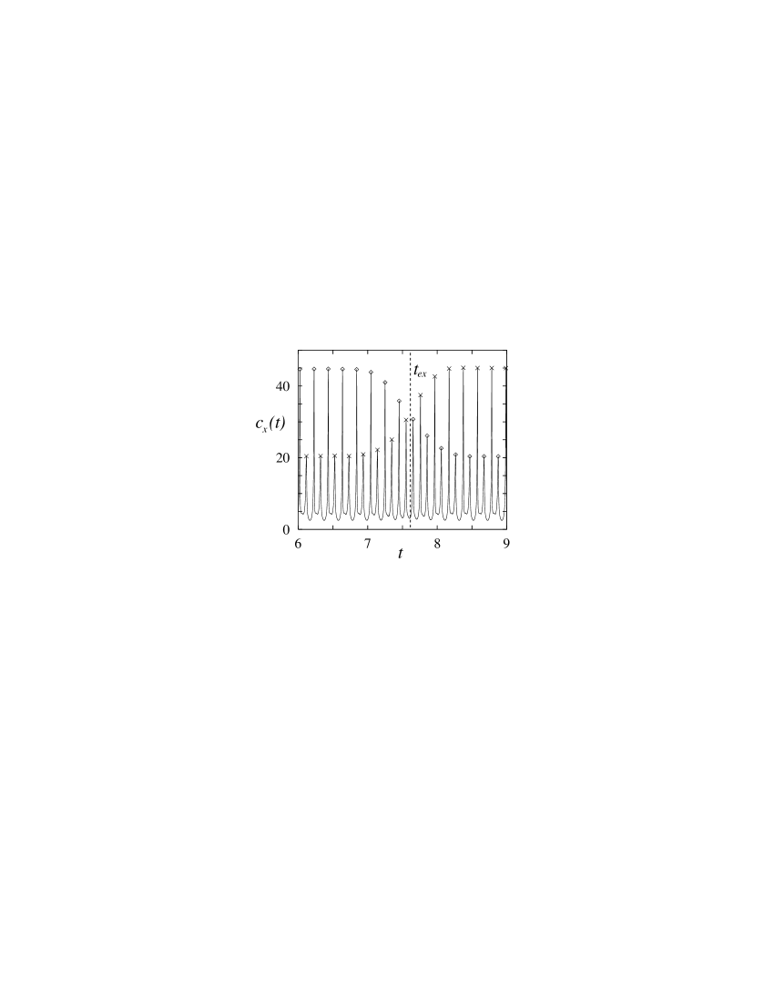
FIG. 7.: Concentration time series $c_{x}(r,t)$ at $r=50$ for the disk-shaped array ($\kappa_{2}=1.544,\;R=80$) showing the loop exchange process. Time unit equals $10^{5}$ $\Delta t$.

For a short period of time near $t_{ex}$ the bands are indistinguishable in phase space and the oscillation is effectively period-1. It is this exchange phenomenon that produces loops that fill the gap between the period-2 bands in the long-time local trajectories (cf. Fig. 5) and contribute to a sparsely scattered “gas”-like density in $G$ (cf. Fig. 6).

An examination of the loop exchanges at different locations in the medium revealed the existence of the following spatio-temporal pattern. At any fixed location the exchange occurs periodically, with period $T_{ex}\approx 55T_{r}$, independent of the position $(r,\theta)$ in the medium. For sufficiently large radii $(r\geq 35)$ this periodicity takes an even stronger form: the entire oscillation pattern, however complex, returns with period $T_{ex}$ to the same configuration.

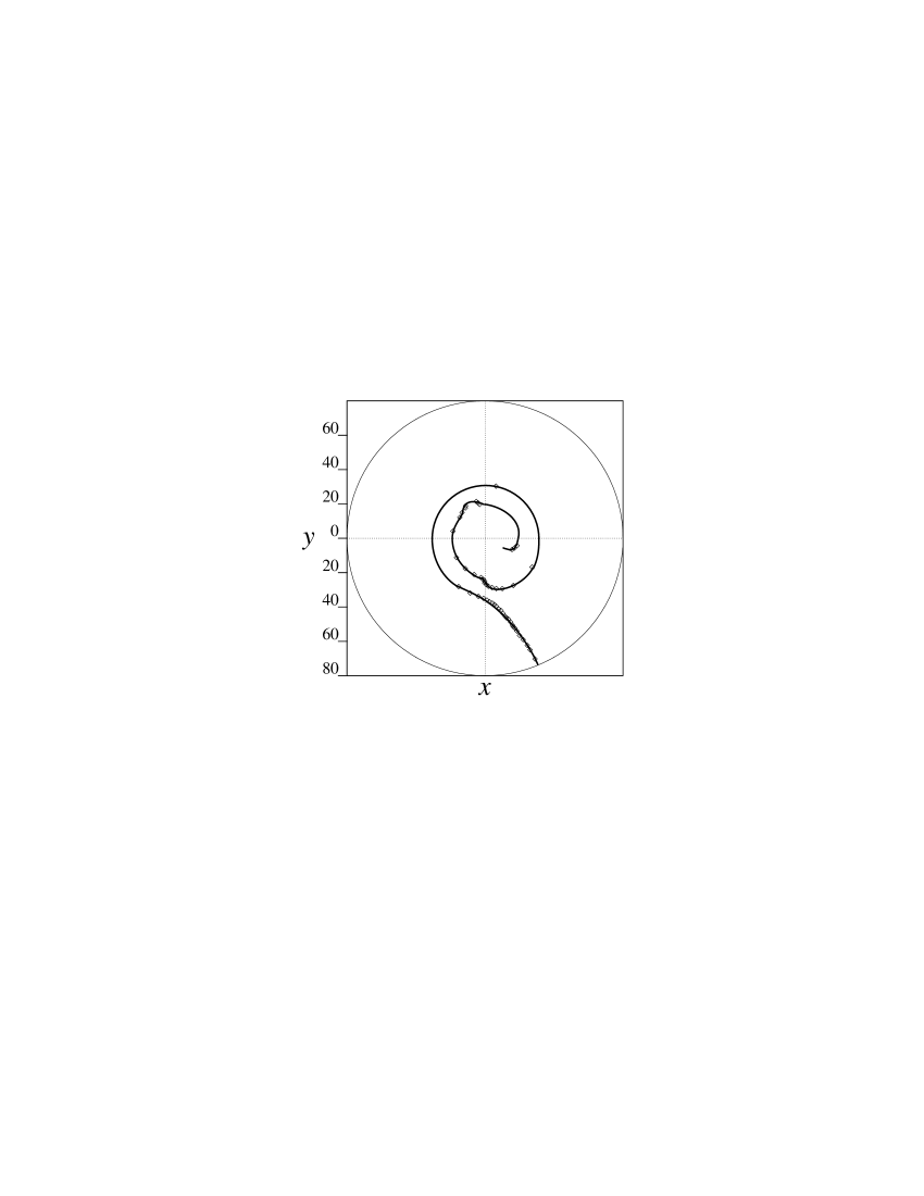
FIG. 8.: Sketch of the $\Omega$ curve for the disk-shaped array ($\kappa_{2}=1.567,\;R=80$). Points where the period-2 band exchange was observed are indicated by diamonds.

This property smoothly disappears as the defect is approached. For two locations ${\bf r}_{1}=(r_{0},\theta_{1})$ and ${\bf r}_{2}=(r_{0},\theta_{2})$ at the same radius $r_{0}$ from the defect but at different angles, the oscillation pattern at one of them, say ${\bf r}_{2}$, can be obtained from the corresponding pattern at ${\bf r}_{1}$ through translation in time by $T_{ex}(\theta_{2}-\theta_{1})/2\pi$, the sign of the translation being defined by ${\rm sign}(\theta_{2}-\theta_{1})$. In view of this observation it is convenient to introduce a coordinate system $(r^{\prime},\theta^{\prime})$ rotating with angular velocity $2\pi/T_{ex}$ relative to the laboratory-fixed coordinate system $(r,\theta)$. In this rotating frame the local dynamics is described by a time-homogeneous pattern, unique for every spatial point ${\bf r^{\prime}}$, and the locations in the medium where loop exchange occurs correspond to points where the local dynamics always has a period-1-like character. The set of loop exchange points constitute a curve $\Omega$ with spiral symmetry which winds twice around the defect (see Fig. 8). The two convolutions of $\Omega$ lie close to circular arcs with radii 19 and 32. This result may be compared with the data obtained from an examination of $G$ (cf. Fig 6). The crossings of the bands of $G$ occur at loci lying on $\Omega$.

Close to the defect the resolution of the loop exchange event is difficult. At $r<18$ the difference between the period-2 bands is comparable to the band thickness and the determination of $\Omega$ for smaller radii becomes impractical. Variation of the system parameters results in a change of the characteristics of $\Omega$; for example, the radius of the domain $R$ does not affect the shape of the $\Omega$ but does change the angular velocity with which the coordinate frame $(r^{\prime},\theta^{\prime})$ in which $\Omega$ is immobile rotates relative to the laboratory-fixed frame $(r,\theta)$. The angular velocity is higher for smaller system sizes: a decrease in $R$ from 80 to 60 reduces the period $T_{ex}$ by a factor of 0.42. A change in the rate constants $\kappa_{i}$ leads to a deformation of $\Omega$, although the identification of $\Omega$ as a set of exchange points remains and it retains the topology of a curve passing from the defect to the boundary. In Sec. V we shall show that the existence of $\Omega$ is essential for the maintenance of spatial continuity in media composed of $2^{n}$-periodic oscillators.

Simulations on a square array with dimension $80\times 80$ (all parameters were the same as for the disk) show that a rotating frame is not necessary to observe the time-homogeneous local dynamics of $C({\bf r}|t_{0},\tau)=C({\bf r}|\tau)$. For this system geometry the $\Omega$ curve is fixed in the medium,

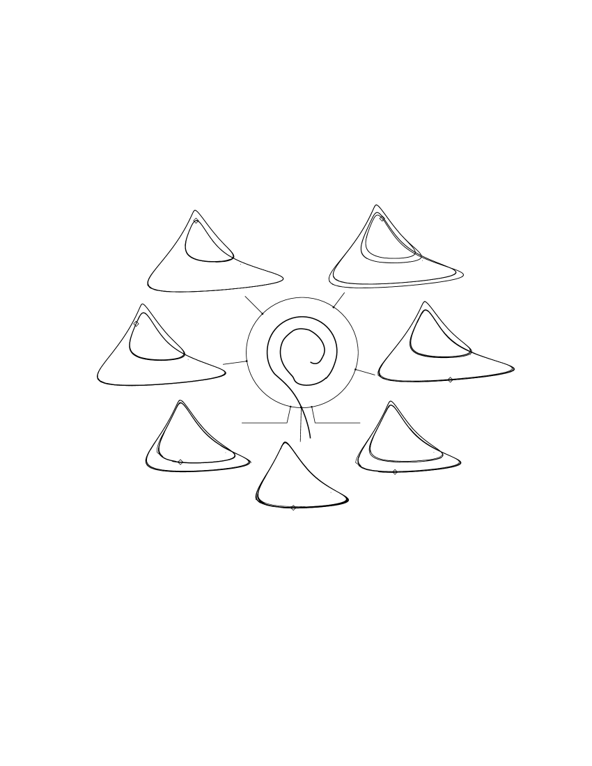
FIG. 9.: Local trajectories calculated on circle with $r=55$ for the square array. All the trajectories are shown on the same scale.

a slight wobbling of the defect (frame origin) being neglected. Figure 9 shows a number of long-time $(\tau\gg T_{r})$ local trajectories on a circle with radius $r_{0}=55$ surrounding the defect in the square domain. One sees a significant dependence of the shape of $C(r_{0},\theta|\tau)$ on the angle $\theta$. The local trajectories range from a period-1 orbit at the intersection with $\Omega$ to the well-established period-4 orbit observed in a certain range of $\theta$. To highlight the loop exchange phenomenon, a particular time instant $t=t^{*}$ is marked on all the trajectories (see Fig. 9). Compare the two $C(r_{0},\theta|\tau)$ at the locations $\theta_{1}$ and $\theta_{2}$ chosen symmetrically on either side of the point $\theta=\theta_{\Omega}$ where the circle intersects $\Omega$. Visual inspection of these orbits shows that their shapes are essentially identical but representative points ${\bf c}(\theta_{1},t^{*})$ and ${\bf c}(\theta_{2},t^{*})$ appear on different period-2 bands of the corresponding orbits. This clearly demonstrates that the period-2 bands do not just approach but indeed pass each other at $\theta=\theta_{\Omega}$, exchanging their positions in phase space. Since it is not necessary to work in a rotating coordinate system in the case of a square domain, one may resolve the fine structure of the local trajectories to a greater degree as can be seen

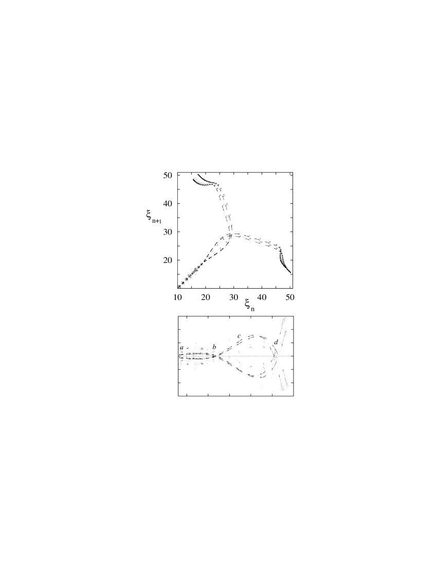
FIG. 10.: Cumulative first return map $G(\theta)$ for the square array ($\kappa_{2}=1.567,\;L=80,\;\theta=0$) (top panel) and a magnification of a portion of its structure (bottom panel). Letters on the bottom panel denote radii for which corresponding portions of $G(\theta)$ are constructed: (a) 9; (b) 19; (c) 25, and (d) 31.

in Fig. 10 (a,b) which shows the cumulative first return map $G(\theta)$ and a magnification of a portion of its structure (compare with Fig. 6). The results show that $G$ is comprised of four branches with the fine structure of period-4 resolved even in the vicinity of the defect ($r=5$ is the closest distance to the defect for which $g(r)$ is shown). Any perturbation of the self-organized pattern of local oscillator synchronization due to irregular motion of the defect, influence of the boundary or the presence of another defect may obliterate subtle fine structure of the local trajectories. In such a circumstance one is able to observe only two gross branches of $G$ and their split nature is not resolvable except for very large $r$. These observations allow one to suppose that the local trajectories may have the same number of fine structure levels everywhere in the medium but the degree to which different levels are resolved in their phase portraits strongly depends on the position in the medium relative to the defect. In view of this hypothesis the phenomenon of spatial period-doubling should not be understood in the literal sense but rather as an enhanced ability to resolve the fine structure with the increase of separation from the defect.

The stationary rotating spiral wave arises from the complex defect-organized cooperation of local oscillators. Each location in the medium develops some site-specific pattern of oscillation which often differs significantly from that of the corresponding rate law attractor and varies substantially from one space point to another. There exists a (possibly rotating) reference frame $(r^{\prime},\theta^{\prime})$, centered on the moving defect, in which local dynamics takes a simple, time-homogeneous form. Each point of the medium in this frame can be assigned a unique oscillatory pattern, different for different spatial points. This allows one to introduce the notion of a defect-organized field associated with $(r^{\prime},\theta^{\prime})$ which specifies the pattern of dynamics in every spatial point of the medium. This field exhibits a complicated architecture lacking of any simple symmetries (which can be easily seen from the shape of the $\Omega$ curve). The slow rotation of this field in disk-shaped arrays restores the circular symmetry of the solution. Although the manner in which different types of local dynamics are distributed in the medium is complex, it is not disordered. Due to the continuity of the medium maintained by the diffusion, it obeys certain topological principles studied in the subsequent sections.

IV Coarse-grained description of local trajectories

In the previous section the phase space shapes of the local trajectories were shown to vary considerably but smoothly from one point in the medium to another. To describe the transformations of these orbits into each other, it is useful to introduce a description which captures only topologically significant changes of phase portraits and disregards unimportant details. To understand the topological principles which determine the global organization of the defect-organized field one also needs a means to compare the time dependence of local trajectories. In this section we present a scheme that allows one to partition the continuum of all the observed local trajectories into a finite number of discrete classes according to their phase space shape and time dependence.

A Representation of attractors by closed braids

Consider a period-$2^{n}$ attractor, $P_{2^{n}}$, consisting of $2^{n}$ loops in the concentration phase space ${\cal P}=(c_{x},c_{y},c_{z})$. Using the cylindrical coordinate system introduced earlier, we may project $P_{2^{n}}$ on the $(\rho,\phi)$ plane preserving its original orientation and 3D character by explicitly indicating whether self-intersections correspond to over or under crossings. Such a projection shows a span of $\phi$ free from crossings where loops are essentially parallel to each other. This span can be used to number loops, say, in the order of their separation from the origin. This procedure maps $P_{2^{n}}$ onto a closed braid ${\bar{B}}_{2^{n}}$ [16]. Figure 11 illustrates the construction of the braid representation for the $P_{4}$ attractor of the WR model.

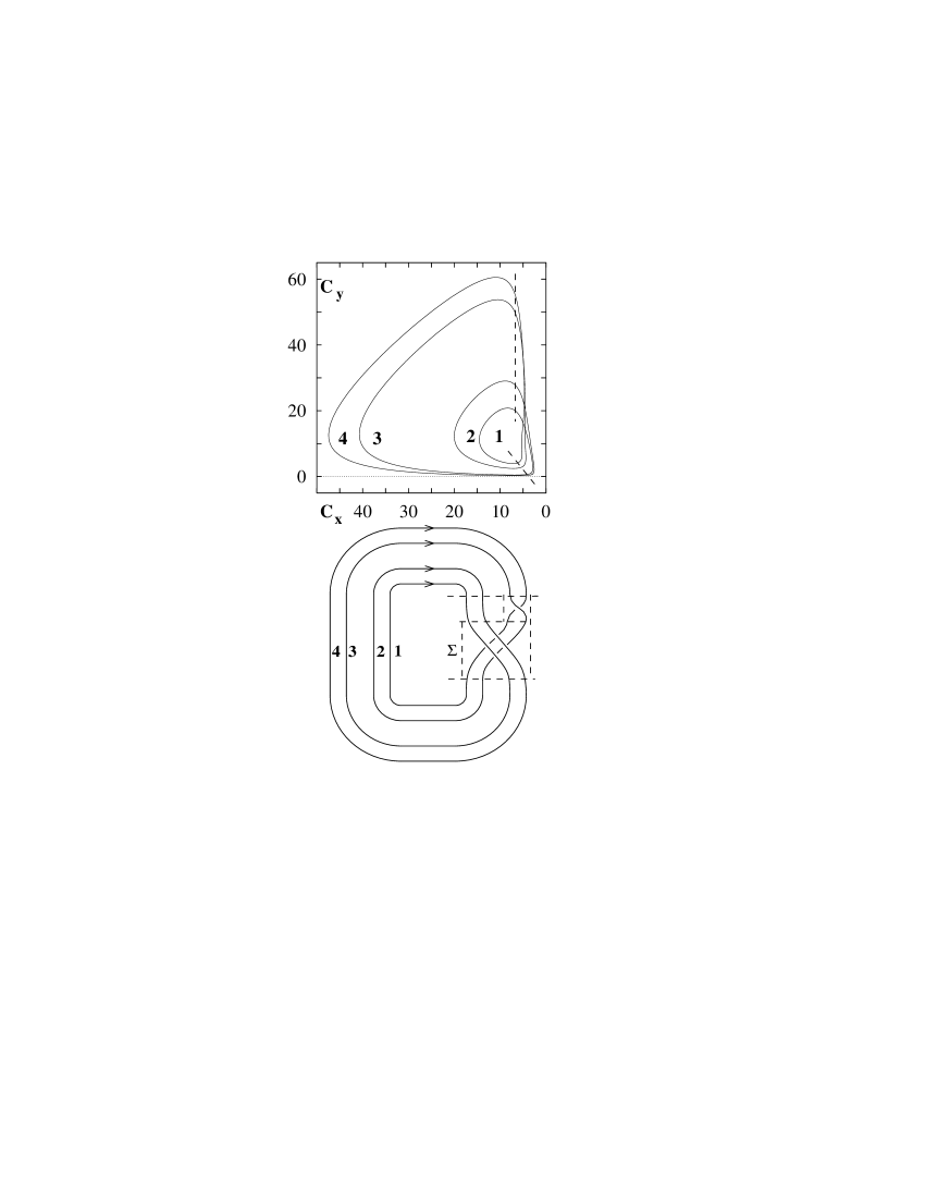
FIG. 11.: Projection of the $P_{4}$ attractor on the $(c_{x},c_{y})$ plane (top panel) and the corresponding closed braid ${\bar{B}}_{4}$ (bottom panel).

It is convenient to subdivide the closed braid ${\bar{B}}_{2^{n}}$ into the open braid $B_{2^{n}}$ (separated by dashed lines in Fig. 11) and its closure where threads run parallel to each other. The direction of the flow on the attractor is indicated by the arrows. Each crossing on the projection of $P_{4}$ corresponds to an elementary braid $\sigma_{i}$ which refers to the fact that thread $i$ overcrosses thread $i+1$ (cf. Fig. 17 in Appendix for notation rule). An under crossing will be designated by ${\sigma}_{i}^{-1}$. A braid may be described by a braid word that gives the order and types of crossings of braid threads. For example, for the closed braid corresponding to $P_{4}$ (cf. Fig. 11) $P_{4}\mapsto{\bar{B}}_{4}=\overline{\sigma_{3}\sigma_{2}\sigma_{1}\sigma_{3}\sigma_{2}}$. The closed braid${\bar{B}}_{2^{n}}$ corresponding to $P_{2^{n}}$ can be represented by several braid words, which can be transformed into one another by a set of allowed moves (see Appendix).

Any braid word representing $P_{2^{n}}$ induces a permutation $\pi^{(n)}_{i}$ describing the order in which loops of $P_{2^{n}}$ are visited during one oscillation period $T_{2^{n}}$. In general, each $P_{2^{n}}$ attractor is represented by several possible $\pi^{(n)}_{i}$, their number growing with $n$; for example, for $P_{2}$ there is only one permutation $\pi^{(1)}_{1}=(^{12}_{21})$ while two permutations $\pi^{(2)}_{1}=(^{1234}_{3421})$ (which corresponds to the braid shown in Fig. 11) and $\pi^{(2)}_{2}=(^{1234}_{4312})$ exist for $P_{4}$. With a given loop numbering convention each braid word represents a unique permutation while one permutation can be induced by many braid words.

B Symbolic representation of periodic orbits

Take two period-$2^{n}$ oscillators whose trajectories ${\bf c}_{1}(t),{\bf c}_{2}(t)$ lie on the same attractor, but which are nevertheless non-identical since at any given time $t$ their dynamical variables are different ${\bf c}_{1}(t)\neq{\bf c}_{2}(t)$. Since the orbits are periodic there is a time $\delta t$ such that ${\bf c}_{1}(t+\delta t)={\bf c}_{2}(t)$ for any $t$. This operation can be formally considered as an action of translation operator ${\cal T}_{\delta t}$ on the trajectory of the first oscillator:

$${\cal T}_{\delta t}\;{\bf c}_{1}(t)={\bf c}_{1}(t+\delta t)={\bf c}_{2}(t).$$ (15)

The concentration time series ${\bf c}(t)$ of the first oscillator then appears to be shifted backward by $\delta t$ relative to that of the time series of the second oscillator if $\delta t>0$ and forward otherwise. Of course, trajectories corresponding to different attractors cannot be made to correspond by such time translations, e.g. $P_{2^{n}}$ attractors described by different permutations $\pi^{(n)}_{i}$ have different patterns of oscillation, but even if two $P_{2^{n}}$ lie in the same $\pi^{(n)}_{i}$ class their actual shapes in ${\cal P}$ may differ significantly.

To compare the local dynamics at different points in the medium one needs to single out the most important characteristic features of the oscillation pattern while discarding unnecessary details. A coarse-grained symbolic description of trajectories appears to be useful for this purpose. We assume that the times $t_{1},t_{2},\ldots,t_{2^{n}}$ at which the trajectory crosses a surface of section $\phi=\phi_{0}$ (see Sec. 2) are approximately equally spaced, independent of the choice of $\phi_{0}$. Thus, the phase point ${\bf c}(t)$ moving along $P_{2^{n}}$ takes approximately the same time $T_{2^{n}}/2^{n}$ to traverse each loop of the attractor.[17] At $t=t_{0}$ let the phase point of the period-$2^{n}$ orbit be on the $j_{0}$-th loop of $P_{2^{n}}$, at $t=t_{0}+T_{2^{n}}/2^{n}$ on the $j_{1}$-th loop, and so on (where $j_{l}\in[1,2^{n}],\;l\in[1,2^{n}],\;j\equiv\!\!\!\!\!\!/\;l$) until at $t=t_{0}+T_{2^{n}}$ the phase point returns to the $j_{0}$-th loop and the pattern $(j_{0},j_{1},\ldots j_{2^{n}})$ repeats. The symbolic string $s_{j}=(j_{0},j_{1},\ldots j_{2^{n}})$ constructed in this way captures the most significant gross features of the oscillation pattern it describes. In this coarse-grained representation the number of possible non-identical trajectories corresponding to a particular $\pi^{(n)}_{i}$ of $P_{2^{n}}$ is finite and the different trajectories are simply given by the $2^{n}$ cyclic permutations of $s_{j}$. Likewise the time translation operators constitute a finite group ${\cal T}_{l},\;l\in[-2^{n-1},2^{n-1})$. They act on the symbolic string representing the orbit to give one of its cyclic permutations.  From its definition it can be easily seen that $\pi^{(n)}_{i}$ serves as a symbolic permutation representation of ${\cal T}_{+1}$ for the corresponding $i$-th permutation class of $P_{2^{n}}$. Indeed, consider as an example a period-4 oscillation whose representative point lies on loop 3 at the reference moment of time $t=t_{0}$. Then for the pattern of oscillation determined by $\pi^{(2)}_{1}$ the state reads $s_{1}=(3241)$. To obtain the new state translated by $T_{4}/4$ backward one acts on $s_{1}$ by the permutation representation $\pi^{(2)}_{1}$ of the ${\cal T}_{+1}$ operator to get

$${\cal T}_{+1}\>s_{1}=\left({}^{{\displaystyle 1234}}_{{\displaystyle 3421}}\right)(3241)=(2413)=s_{2},$$ (16)

which correctly describes the result of the shift of the initial state $s_{1}$.

V Global organization of medium

A Period-1 regime

We now return to the spatially distributed medium and begin by reviewing some properties of the local dynamics in the vicinity of a stable defect with topological charge $n_{t}=\pm 1$ in a period-1 oscillatory medium. Consider a cyclic path $\Gamma=\{r=r_{0}>r_{max},\theta\in[0,2\pi)\}$ surrounding the defect. Here $r_{max}$ is a radius such that for all $(r,\theta),r>r_{max},\>\theta\in[0,2\pi)$ the shape of the local orbit in phase space ${\cal P}$ is independent of $(r,\theta)$ and closely approximates that of the period-1 attractor of the mass action rate law (see Sec. II). If one starts at an arbitrary point $(r_{0},\theta_{0})\in\Gamma$ one finds that the instantaneous local phase $\phi({\bf r},t)$ changes by $2\pi$ or $-2\pi$ (depending on the sign of the topological charge) along $\Gamma$. Let us now fix a particular time instant $t=t^{*}$ and construct the set of points ${\cal S}=\{{\bf c}({\bf r},t^{*}),r\in\Gamma\}$ as a phase space image of instantaneous concentrations at points lying on $\Gamma$.

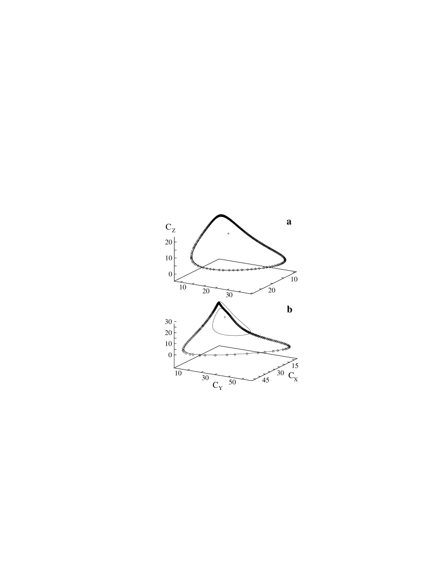
FIG. 12.: ${\cal S}$-curves (shown by diamonds) constructed for $\Gamma$ with $r_{0}=55$ in period-1 oscillatory ($\kappa_{2}=1.420$) (a) and chaotic ($\kappa_{2}=1.567$) (b) media. Solid curves represent short time local trajectories on $\Gamma$.

The property of a defect (10) and the continuity of the medium insure that ${\cal S}$ is a simple closed curve winding once around ${\bf c}^{*}$. Figure 12(a) shows the ${\cal S}$-curve constructed for the contour $\Gamma$ with radius $r_{0}=55,\,r_{0}>r_{max}$ in a period-1 oscillatory medium with $\kappa_{2}=1.420$. Since all the points on the ${\cal S}$-curve lie at the same time on the local trajectories $C({\bf r}|t_{0},\tau),\,{\bf r}\in\Gamma$ with $t^{*}\in[t_{0},t_{0}+\tau]$, and for $\Gamma$ with $r_{0}>r_{max}$ all the local trajectories are the same and approximated by the period-1 attractor of the system (5), the ${\cal S}$-curve simply coincides with this attractor for any $t^{*}$ (cf. Fig. 12(a)). The ${\cal S}$-curve constructed for an arbitrary simple closed path encircling the defect in the medium possesses the same property as long as the path lies in the open region $r>r_{max}$.

This result can be reformulated in terms of time translations of local trajectories as follows. Let the local trajectory $C(r_{0},\theta_{0}|t_{0},\tau)$ at the point $(r_{0},\theta_{0})\in\Gamma$ be taken as a reference, then all of the local trajectories on $\Gamma$ can be obtained through the translation of $C(r_{0},\theta_{0}|t_{0},\tau)$ by some time $\delta t(\theta-\theta_{0})$ (see Sec. IV). The condition (10) implies that $\delta t(\theta-\theta_{0})$ is a monotonically increasing (decreasing) function such that $\delta t(2\pi)=\pm T_{1}$ where $T_{1}$ is the period of oscillation and the sign is that of $n_{t}$. Thus, the oscillation pattern is continuously time shifted along $\Gamma$ such that upon return to the initial point it has experienced translation by the period.

B Period-$2^{n}$ regime

For $2^{n}$-periodic and chaotic media property (10) holds where $\phi({\bf r},t)$ should be understood as the angle variable introduced in Sec. II. This can be seen from the following argument. Take a period-2 medium with rate constants chosen in the vicinity of the bifurcation from period-1 to period-2 such that the attractor $P_{2}$ of (5) lies infinitesimally close to $P_{1}$ from which it bifurcated. Due to the continuity of the solutions of the reaction-diffusion equation (9), the value of $\oint\phi({\bf r},t)\;d{\bf l}$ cannot change abruptly when the bifurcation parameter is changed through the period-doubling bifurcation. This implies that the ${\cal S}$-curve constructed for a contour $\Gamma$ in a period-$2^{n}$ medium, as in case of a simple period-1 medium, is a closed curve which loops once around ${\bf c}^{*}$ in phase space. This is illustrated in panel (b) of Fig. 12 which shows ${\cal S}$ for contour $\Gamma$ with radius $r_{0}=55$ in medium with $\kappa_{2}=1.567$ and time $t=t^{*}$. Recall again that the points of the ${\cal S}$ curve have to lie on the local trajectories $C({\bf r}|t_{0},\tau),\,{\bf r}\in\Gamma$ (cf. Fig. 9 where points designated by diamonds lie on ${\cal S}$ for the chosen time moment and contour shown in the figure). Since the local trajectories in a period-$2^{n}$ medium loop several times around ${\bf c}^{*}$, the curve ${\cal S}$ which winds only once $(n_{t}=\pm 1)$ around ${\bf c}^{*}$ cannot span the entire local trajectory as is the case for a period-1 medium. As one sees from Fig. 12(b) ${\cal S}$ follows the larger loop of the local trajectory, which for $\Gamma$ with $r_{0}=55$ is typically a period-2 orbit (cf. Fig. 9), and instead of making the second turn on the smaller loop, it crosses the gap between the loops and closes on itself. Although the shape of ${\cal S}$ changes with time (see [7] for details), for any $t^{*}$ there exist segments of ${\cal S}$ which connect different loops of local trajectories. This behavior of the ${\cal S}$ curves would be impossible if loop exchanges were nonexistent. The analysis shows that the segments of ${\cal S}$ covering the gaps between the loops of the local trajectories are images of points on $\Gamma$ which lie close to the intersection with the $\Omega$ curve. Thus, the loop exchanges observed in period-$2^{n}$ media are necessary to reconcile the contradiction between the one-loop topology of the ${\cal S}$ curves determined by the presence of a defect and the multi-loop topology of the local trajectories determined by the local rate law.

The change of the local trajectories along the contour $\Gamma$ in period-$2^{n}$ media can be considered in terms of time translations if one adopts a generalization of the translation operation in the following way. In a period-2 medium let the contour $\Gamma$ and the reference point $(r_{0},\theta_{0})\in\Gamma$ be chosen so that $\Gamma$ intersects the $\Omega$ curve in the single point $(r_{0},\theta_{\Omega})$ and suppose that these points are sufficiently separated from each other. Since the shapes of the local orbits change significantly along any closed path surrounding a defect (cf. Fig. 9) these trajectories cannot be made to coincide by time translation as this operation is defined in Sec. IV. Nevertheless, the general features of the temporal pattern of the trajectories are preserved (e.g. sharp maxima in $c_{i}(t)$ time series) and for two

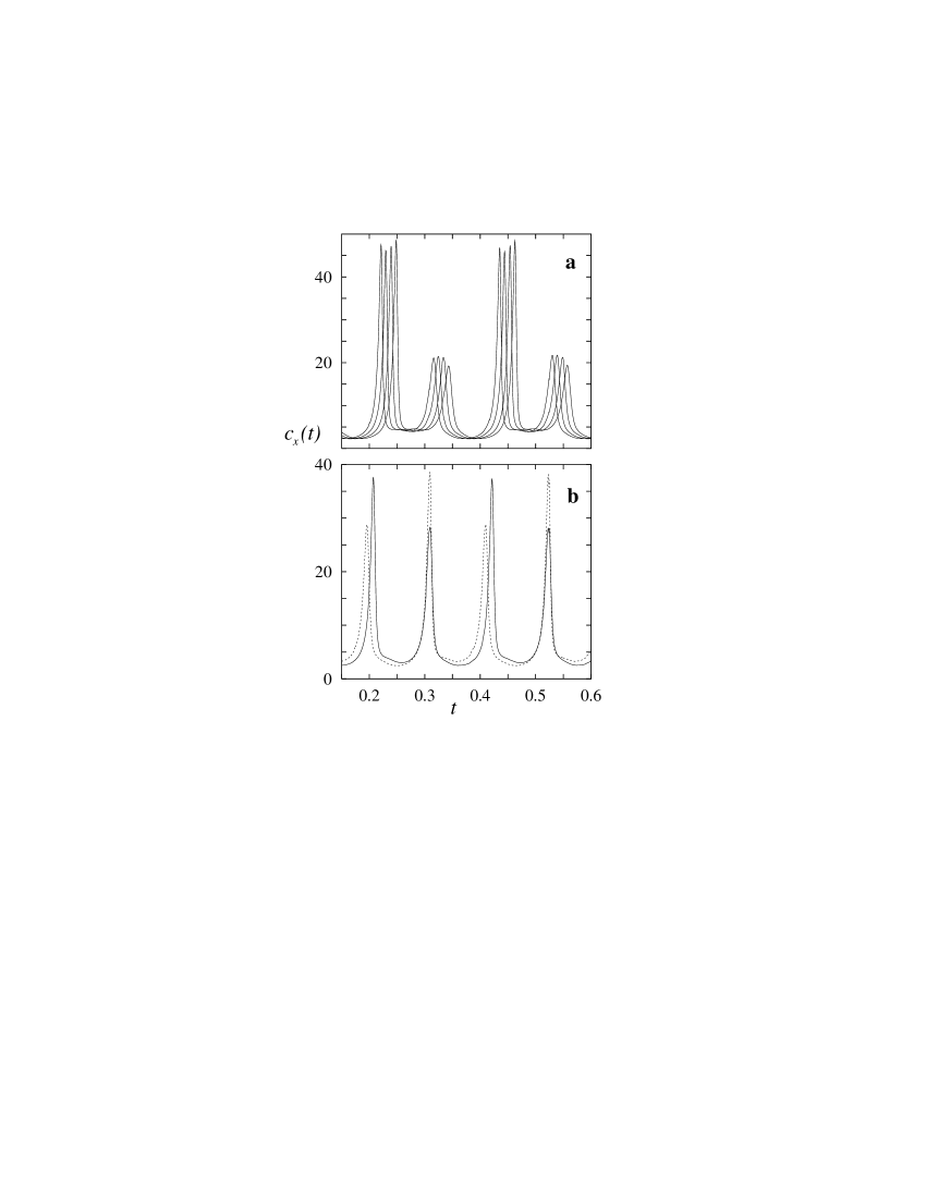
FIG. 13.: Period-2 local concentration time series $c_{x}({\bf r},t)$ calculated on a cyclic path $\Gamma$ surrounding the defect: (a) series sampled at four consecutive locations separated by $\delta\theta=30^{o}$; (b) two series sampled at locations chosen symmetrically on either side of the intersection with the $\Omega$ curve.

locations $(r_{0},\theta_{1})$ and $(r_{0},\theta_{2})$ one is able to find a time shift $\Delta t(\theta_{1},\theta_{2})$ such that some measure of the deviation between the trajectories, say,

$$M(\Delta t(\theta_{1},\theta_{2}))=\int_{t_{0}}^{t_{0}+\tau}|{\bf c}^{(1)}(t+\Delta t)-{\bf c}^{(2)}(t)|\>dt,$$ (17)

is minimized. Choosing the local trajectory $C(r_{0},\theta_{0}|t_{0},\tau)$ as a reference and comparing it to all the other local orbits on $\Gamma$ one is able to define the time shift function $\delta t(\theta-\theta_{0})\equiv\Delta t(\theta,\theta_{0})$. The shift function $\delta t(\theta-\theta_{0})$ increases (or decreases) monotonically and almost linearly (see Fig. 13(a)) with $d(\delta t)/d\theta\approx T_{2}/2\cdot 2\pi$ everywhere on $\Gamma$ except for a small neighborhood of $\theta=\theta_{\Omega}$ where it exhibits break. Indeed, the loop exchange at $\theta=\theta_{\Omega}$ causes the discontinuity of $\delta t(\theta-\theta_{0})$. At $\theta=\theta_{\Omega}$ both loops of the local orbit become equivalent and the oscillation is effectively period-1 with period $T_{1}=T_{2}/2$. Since the loops exchange at $\theta=\theta_{\Omega}$, to find the best match (17) between local trajectories sampled at points $(r_{0},\theta_{\Omega}-\varepsilon)$ and $(r_{0},\theta_{\Omega}+\varepsilon)$, one needs to translate one of the trajectories by $\delta t=T_{1}+O(\varepsilon)$. This can be easily seen in Fig. 13(b) which displays two $c_{x}(t)$ series calculated at spatial points lying $\theta-\theta_{\Omega}=\pm 10^{o}$ on either side of $\theta_{\Omega}$ on $\Gamma$.

C Trajectory transformations along $\Gamma$

The transformation of local trajectories along $\Gamma$ can be imagined to occur a result of two separate processes. Suppose everywhere on $\Gamma$ except $\theta=\theta_{\Omega}$ the shape of the local trajectories in ${\cal P}$ is the same and is equivalent to that of $C(r_{0},\theta_{0}|t_{0},\tau)$. Then all the other local trajectories $C(r_{0},\theta|t_{0},\tau),\;\theta\in[0,2\pi),\theta\neq\theta_{\Omega}$ can be found by time translation of $C(r_{0},\theta_{0}|t_{0},\tau)$ by $\delta t(\theta-\theta_{0})=T_{2}(\theta-\theta_{0})/2\cdot 2\pi$. Assume that all the deformations of the phase space portrait of the local trajectory which take place along $\Gamma$, including the exchange of loops, occur at the point $\theta=\theta_{\Omega}$ so that the passage through $\theta_{\Omega}$ shifts the oscillation by $\delta t_{p}=T_{1}=T_{2}/2$. Then the result of the continuous time translation that occurs during $2\pi$ circulation along $\Gamma$ may be described by the action of the ${\cal T}_{n_{t}}$ operator $(n_{t}=\pm 1)$, while the result of the loop exchange is described by the operator ${\cal T}_{-n_{t}}$. [18] The total transformation of the local oscillation after a complete cycle over $\Gamma$ is equivalent to the identity transformation and thus the result is in accord with continuity of the medium. If one makes the assumption that loop exchange does not occur on some contour $\Gamma$ encircling a defect with $|n_{t}|=1$, the time shift function $\delta t(\theta-\theta_{0})$ becomes monotonic and continuous everywhere on $\Gamma$. As a result one arrives at the incorrect conclusion that starting from the point $(r_{0},\theta_{0})$ with the oscillation pattern symbolically represented by the string $s_{1}$, say $s_{1}=(12)$, and moving along $\Gamma$ in the clockwise direction one returns to the same point $(r_{0},\theta_{0}+2\pi)\equiv(r_{0},\theta_{0})$ but with the oscillation pattern shifted by $T_{2}/2$ and given by $s_{2}=(21)\neq s_{1}$. Note that this contradiction does not arise in the period-1 oscillatory medium where circulation over any closed path encircling a defect results in the translation by the entire period which automatically satisfies the continuity principle. Thus the necessity of loop exchanges in period-$2^{n}$, $n>0$ media with a topological defect demonstrated earlier in this section in terms of ${\cal S}$-curves is now explained in terms of time translations.

The results for the period-2 medium can be generalized for any $n>1$ using the following hypothesis.  From the main property of a topological defect (10) it follows that integration of an infinitesimal continuous shift $d(\delta t)$ over any closed path surrounding a defect results in a total shift by $\pm T_{2^{n}}/2^{n}$ and can be symbolically described by the ${\cal T}_{n_{t}}$ operator. Numerical simulations demonstrate the existence of time translation discontinuity points such that sum of $\delta t$ jumps over these points amounts to a shift of $\mp T_{2^{n}}/2^{n}$ described by the ${\cal T}_{-n_{t}}$ operator. The locations of these points in the medium can be identified with the $\Omega$ curve and the origin of the time translation discontinuities with the loop exchange phenomenon. The relation (A10) of the Appendix connects translations and loop exchanges and allows one to predict the number and the kind of loop exchanges necessary to perform the required ${\cal T}_{-n_{t}}$ translation.

D Examples

Consider again the square $80\times 80$ array with rate constants corresponding to chaotic regime ($\kappa_{2}=1.567$). As period-4 fine structure is the highest level of local organization resolved in the medium, it is sufficient to use the formalism developed above for $P_{4}$ to describe the local dynamics. The analysis shows that in the bulk of the medium the oscillation is given by the $\pi^{(2)}_{1}=(^{1234}_{3421})$ pattern. [19] Using this data and the results presented in the Appendix one can easily enumerate all the sequences of exchanges resulting in ${\cal T}_{+1}$ translation. Indeed, one should expect either exchange of loops 3 and 4 followed by the exchange of period-2 bands $(^{1234}_{3412})$ or first the period-2 bands exchange followed by exchange of loops 1 and 2. Figure 14 is a schematic representation of the medium with a negatively charged $(n_{t}=-1)$ defect in the center and the $\Omega$ curve displayed.

Consider the change of the oscillation pattern along ray $ABC$ emanating from the defect as the value of $r$ increases (see Fig. 10 for the cumulative first-return map constructed for this ray). The pattern of oscillation $s_{A}=(4132)$ corresponding to permutation $\pi^{(2)}_{1}=(^{1234}_{3421})$ can be followed from $r=5$ to $r=19$ where the period-2 bands undergo exchange. This results in the switch to the oscillation pattern described by $\pi^{(2)}_{2}=(^{1234}_{4312})$ seen at $r=21$. The pattern $\pi^{(2)}_{1}$ is restored after loops 1 and 2 exchange at $r=22$ and and this pattern persists until another exchange occurs at $r=28$.

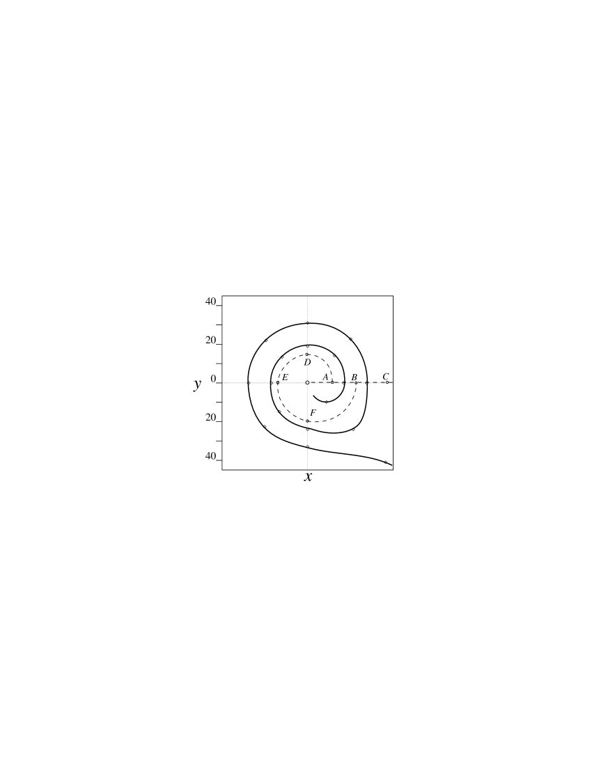
FIG. 14.: Sketch of the $\Omega$ curve for the square array ($\kappa_{2}=1.567,\;L=80$). The points were obtained from simulations. The ray $ABC$ intersects $\Omega$ at locations with radii 20 and 31.

Using translation operator ${\cal T}_{+1}$ one can express the transition of the state $s_{A}$ ($r<20$) through the sequence of loop exchanges described above to the state $s_{B}=(1324)$ (for $22<r<28$) as $s_{B}={\cal T}_{+1}s_{A}$. The same shift can be achieved by continuous translation along the path $ADEFB$ which does not intersect $\Omega$ but winds once counter-clockwise around the defect. The $c_{x}(t)$ time series at points $A,D,E,F$ and $B$ are displayed in Fig. 15 and demonstrate that this is the case.

FIG. 15.: Concentration time series $c_{x}({\bf r},t)$ calculated at points $A,D,E,F,B$ of the square array shown in Fig. 15.

Continuing to advance along the ray $ABC$, one finds that at $r=28$ loops 3 and 4 exchange and oscillation switches once more to the state corresponding to $\pi^{(2)}_{2}$. After the period-2 band exchange at $r=32$ the pattern corresponding to $\pi^{(2)}_{1}$ is reinstated and remains unchanged for all $r>32$. Again the oscillation at $r>32$, described symbolically by $s_{C}=(3241)$, appears to be shifted by $T_{4}/4$ relative to $s_{B}$ and by $T_{4}/2$ relative to $s_{A}$.

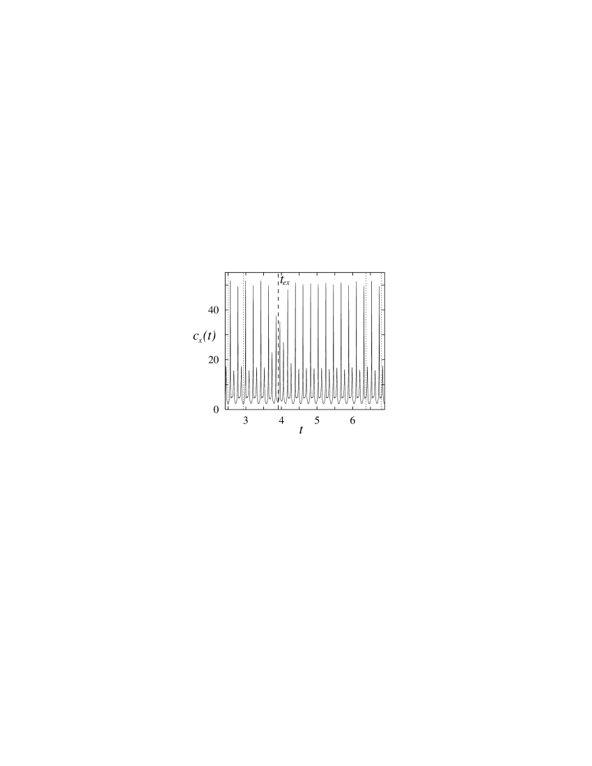
FIG. 16.: Segment of the concentration time series $c_{x}(r,t)$ calculated for the disk-shaped array ($\kappa_{2}=1.567,\;R=80$) at $r=76$ showing the $T_{4}/4$ time shift of the oscillation pattern (see explanation in the text).

The existence of a $T_{4}/4$ shift after crossing $\Omega$ can also be seen from the results for the disk-shaped array with $R=80$. Figure 16 shows a segment of the $c_{x}({\bf r},t)$ time series sampled in a fixed frame $(r,\theta)$ at $r=76$. In this coordinate system $\Omega$ slowly rotates clockwise (again $n_{t}=-1$) with period $T_{ex}$. Two time windows each of length $T_{4}$ marked by dotted lines and separated by $\Delta t=8T_{4}$ allow one to see how the oscillation state (4132) is substituted by its forward $T_{4}/4$ translation (2413) after the $\Omega$ curve passes the observation point at $t=t_{ex}$.

VI Conclusions

General principles underlie the organization of $2^{n}$-periodic or chaotic media supporting spiral waves. As in simple oscillatory media, the core of a spiral is a topological defect which acts as an organizing center determining dynamics in its vicinity; however, the structural organization of the medium that arises from the existence of the defect is far more complicated. Due to the absence of a conventional definition of phase for oscillations more complex than period-1, the identification of a defect in terms of the relation (10) is not obvious and requires the introduction of (often model-dependent) phase substitutes which for some systems may be provided by angle variables. Despite the complications with the definition of phase, one can identify a defect in terms of local trajectories. Indeed, as one moves away from the defect the local dynamics takes the form of a progression of period-doubled orbits, from near harmonic, small-amplitude, period-1 orbits to “noisy” period-$2^{l}$ orbits, where $l$ is a function of variables such as diffusive coupling and the system size and shape.

The presence of a defect imposes topological constraints on the global organization of medium as well. As was shown above, when $2^{n}>n_{t}$ the $2^{n}$-loop structure of the local trajectories conflicts with the period-$n_{t}$ structure of the ${\cal S}$-curve and a complex, asymmetric, spatial pattern of local dynamics, the defect-organized field, arises as a result of the necessity to maintain the continuity of the medium. The most prominent characteristic feature of this field is the $\Omega$ curve defined as the set of points where the local dynamics most closely resembles period-1. This signals the exchange of period-2 bands. If the local trajectories possess structure finer than period-2, other loop exchanges leading to more subtle changes in the local orbits can be found in the vicinity of $\Omega$. The net result of these exchanges is to produce a time shift of the trajectories which compensates for the smooth time translation accumulated on continuous paths. Since the topological continuity must be observed on any arbitrarily large closed path encircling a defect and, therefore, this contour has a point of intersection with $\Omega$, a single defect in a period-$2^{n}$ $(n>0)$ medium cannot be localized.

We point out again that many of the phenomena we have discussed above are not dependent on the existence of a period-doubling cascade or chaotic local dynamics, although this is the case we have analysed in detail. Reaction-diffusion systems with local complex periodic orbits in phase space dimensions higher than two should exhibit similar features when they support spiral waves. It should be possible to experimentally probe the phenomena described in this paper. The appropriate parameter regime can be determined from investigations of well-stirred systems. For example, period-doubling and chaotic attractors have been observed in the Belousov-Zhabotinsky reaction. [20] If the spiral wave dynamics is then studied in a continuously-fed-unstirred reactor [21], one should be able to observe the characteristics of the spiral dynamics and the loop exchange process that serve as signatures of the phenomena described above.

VII Acknowlegements

We thank Peter Strizhak for his interest in this work and helpful comments. This work was supported in part by a grant from the Natural Sciences and Engineering Research Council of Canada and by a Killam Research Fellowship (R.K.).

A Braid moves and loop exchange operators

In this appendix we make use of the projection of the period-doubled attractors $P_{2^{n}}$ onto closed braids ${\bar{B}}_{2^{n}}$ (see Sec. IV) to show how loop exchanges affect the pattern of oscillation. We demonstrate that those combinations of loop exchanges that produce identity transformations of $P_{2^{n}}$ result in nontrivial time translations of trajectories.

Each closed braid ${\bar{B}}_{2^{n}}$ is represented by a set of non-identical braid words with their number rapidly growing with $n$. Without violation of the topology of ${\bar{B}}_{2^{n}}$ they can be transformed into one another by the following set of moves (see, e.g. [16]) :

1. commutation relation, $\sigma_{i}\sigma_{j}=\sigma_{j}\sigma_{i},\;\;|i-j|\geq 2$;

2. type 2 Reidemeister move, $\sigma_{i}\sigma_{i}^{-1}=\sigma_{i}^{-1}\sigma_{i}={\bf 1}$;

3. type 3 Reidemeister move, $\sigma_{i}\sigma_{i+1}\sigma_{i}=\sigma_{i+1}\sigma_{i}\sigma_{i+1}$;

4. first Markov move, $\sigma_{i}\Sigma\sigma_{i}^{-1}=\sigma_{i}^{-1}\Sigma\sigma_{i}=\Sigma,\;\Sigma\in B$;

where $B$ is a set of open braids. While the first three rules are common for all braids, rule 4 is specific for closed braids. Indeed, it can be written in the form $\sigma_{i}\Sigma=\Sigma\sigma_{i}$ which, for elementary braids $\sigma_{i}$, corresponds to moving $\sigma_{i}$ around ${\bar{B}}_{2^{n}}$ resulting in the exchange of the closed braid loops (cf. Fig. 17(d)). Type 1 Reidemeister (or second Markov) moves are not allowed since they do not preserve the number of loops, an essential feature of $P_{2^{n}}$

FIG. 17.: Conventional designations and basic braid moves: (a) definition of elementary braids $\sigma_{i}$ and $\sigma_{i}^{-1}$; (b) type 2 Reidemeister move; (c) type 3 Reidemeister move, and (d) first Markov move ($\Sigma$ represents arbitrary braid).

attractors. While rules 1, 2 and 3 do not affect $\pi^{(n)}_{i}$, the first Markov move does (except for the degenerate case of $P_{2}$ which is represented by the single permutation $\pi^{(1)}_{1}$). Thus any number of rearrangements affecting only the braid $B_{2^{n}}$ of the closed braid ${\bar{B}}_{2^{n}}$ leave the braid word in the same permutation class $\pi^{(n)}_{i}$, while each application of the first Markov move yields a new permutation class.

1 Loop exchanges for $P_{2}$ and $P_{4}$

We now examine how the loop exchanges influence the patterns of oscillation for the period-2 and period-4 attractors. For $P_{2}$ one has only the single braid word $\sigma_{1}(\sigma_{1}^{-1})$ and the single permutation $\pi^{(1)}_{1}=(^{12}_{21})$ induced by $\sigma_{1}$. Two different symbolic states $s_{1}=(12)$ and $s_{2}=(21)$ are possible for the period-2 oscillation with respect to some fixed time frame. We introduce an operator $A^{(1)}_{1}$ whose action on the closed braid representing $P_{2}$ is to move $\sigma_{1}$ by $2\pi$ in a direction opposite to the flow. The result of the action of this operator, which is the first Markov move for $\Sigma={\bf 1}$, is to leave the attractor $P_{2}$ unchanged; however, one finds that loops 1 and 2 have exchanged their locations in phase space. In the time series for the dynamical variable $c_{i}(t)$ the exchange can be seen as a substitution of taller maxima (2) by shorter maxima (1) and vice-versa. If this process is followed in time it produces the characteristic pattern shown in Fig. 7. Thus, application of $A^{(1)}_{1}$ to $P_{2}$ induces a transformation of the oscillation state $s_{1}$ into $s_{2}$ and vice-versa. This can be symbolically described as an action of an exchange operator ${\cal A}^{(1)}_{1}$ represented by the permutation $(^{12}_{21})$ :

$${\cal A}^{(1)}_{1}\>s_{1} = \left({}^{{\displaystyle 12}}_{{\displaystyle 21}}\right)(12)=(21)=s_{2},$$ (A1)

$${\cal A}^{(1)}_{1}\>s_{2} = \left({}^{{\displaystyle 12}}_{{\displaystyle 21}}\right)(21)=(12)=s_{1}.$$ (A2)

One sees that the action of ${\cal A}^{(1)}_{1}$ is equivalent to that of ${\cal T}_{+1}$ which translates the oscillation pattern by half a period. The inverse of the braid operator $A^{(1)}_{1}$ can be introduced in an analogous way as an operator moving $\sigma_{1}$ along the direction of the flow. It corresponds to an exchange operator $({\cal A}^{(1)}_{1})^{-1}={\cal T}_{-1}$ acting on strings. Since for $P_{2}$ application of ${\cal T}_{+1}$ or ${\cal T}_{-1}$ results in essentially the same states the sign of the shift is chosen to maintain consistency with corresponding operators for $P_{2^{n}}$, $n>1$. Double application of ${\cal A}^{(1)}_{1}$ results in translation by a full period and thus in the identity operator

$$({\cal A}^{(1)}_{1})^{2}=({\cal A}^{(1)}_{1})^{-2}={\bf 1}.$$ (A3)

The $P_{4}$ attractor possesses a richer set of transformations. Since under coarse-graining braid words which induce the same $\pi^{(n)}_{i}$ are indistinguishable, we can single out two essential representatives $\Sigma_{1}=\sigma_{3}\Sigma$ for $\pi^{(2)}_{1}=(^{1234}_{3421})$ and $\Sigma_{2}=\sigma_{1}\Sigma$ for $\pi^{(2)}_{2}=(^{1234}_{4312})$, where $\Sigma$ stands for $\sigma_{2}\sigma_{1}\sigma_{3}\sigma_{2}$. Let $A^{(2)}_{1}$ be an operator on ${\bar{B}_{2}}$ which moves the double-thread crossing (cf. large dashed box in Fig. 11) $\Sigma$ by $2\pi$ in the direction opposite to the flow, analogous to the action of $A^{(1)}_{1}$ on $\sigma_{1}$ for ${\bar{B}_{2}}$. In fact, the action of $A^{(2)}_{1}$ can be seen as an exchange of the period-2 bands of $P_{4}$, each consisting of two period-4 loops. Unlike $A^{(1)}_{1}$ the operator $A^{(2)}_{1}$ alternates braid words and the corresponding pattern-defining permutations $\Sigma_{1},\pi^{(2)}_{1}\stackrel{{\scriptstyle A^{(2)}_{1}}}{{\longleftrightarrow}}\Sigma_{2},\pi^{(2)}_{2}$. The application of $A^{(2)}_{1}$ induces transformations of symbolic strings $s_{j}$ which again can be described by the action of an exchange operator ${\cal A}^{(2)}_{1}$ represented by the permutation $(^{1234}_{3412})$. Due to the apparent similarity of action of $A^{(1)}_{1}$ and $A^{(2)}_{1}$ on the corresponding attractors, ${\cal A}^{(2)}_{1}$ inherits the algebraic properties of ${\cal A}^{(1)}_{1}$. Indeed, ${\cal A}^{(2)}_{1}$ produces identity operator when applied twice and, thus, is equal to its inverse.

Finer rearrangement of the $P_{4}$ loop structure is provided by the action of $A^{(2)}_{2}$ defined as an operator which moves the single crossing (enclosed in the smaller box in Fig. 11) by $2\pi$ in the direction opposite to flow.  From the structure of ${\bar{B}_{4}}$ one sees that after application of $A^{(2)}_{2}$ the single crossing does not return to the same location in ${\cal P}$ but appears on the other period-2 band; thus, braid words and $\pi^{(n)}_{i}$ permutations alternate. Depending on the initial state, the application of $A^{(2)}_{2}$ results in different loop exchanges. In the case of $\Sigma_{1}=\sigma_{3}\Sigma$ action of $A^{(2)}_{2}$ leads to the exchange of loops $3$ and $4$ and results in the string transformation described by the exchange operator ${\cal A}^{(2)}_{2}$ with symbolic representation $(^{1234}_{1243})$. When it acts on $\Sigma_{2}=\sigma_{1}\Sigma$ it exchanges loops 1 and 2 and the permutation representation of ${\cal A}^{(2)}_{2}$ changes to $(^{1234}_{2134})$. The inverse of $A^{(2)}_{2}$ moves the single crossing along the flow and produces opposite results; i.e., acting on $\Sigma_{1}$ it leads to $1\leftrightarrow 2$ exchange and when applied to $\Sigma_{2}$ it results in the exchange $3\leftrightarrow 4$.

Note the difference between action of $A^{(n)}_{i}$ on braids and the action of exchange operators ${\cal A}^{(n)}_{i}$ on symbolic strings. While several operations $A^{(n)}_{i}$ applied to the same initial braid word lead to equivalent final words (e.g. $A^{(2)}_{1}$ and $A^{(2)}_{2}$) the resulting loop exchanges and, thus their permutation descriptions, can be quite different ($(^{1234}_{3412})$ and $(^{1234}_{1243})$ for the example chosen). Consequently, compositions of braid operations returning the braid ${\bar{B}}_{2^{n}}$ to its initial state (e.g. $A^{(2)}_{2}\circ A^{(2)}_{2}$) may induce nontrivial translations of $s_{j}$. To demonstrate this let $({\cal A}^{(2)}_{2})^{2}$ act on the trial state $s_{1}=(3241)$. Applying the rules one obtains

$$({\cal A}^{(2)}_{2})^{2}\>s_{1}=\left({}^{{\displaystyle 1234}}_{{\displaystyle 2134}}\right)\left({}^{{\displaystyle 1234}}_{{\displaystyle 1243}}\right)(3241)=(4132)={\cal T}_{+2}\>s_{1},$$ (A4)

thus relating the simultaneous loop exchange $(13)\leftrightarrow(24)$ with translation of the period-4 oscillation by half of a period. This implies as well that application of ${\cal A}^{(2)}_{2}$ four times results in the identity string transformation $({\cal A}^{(2)}_{2})^{4}={\cal T}_{+4}={\bf 1}$ and, therefore, $({\cal A}^{(2)}_{2})^{-1}=({\cal A}^{(2)}_{2})^{3}$. Compositions of braid operators $A^{(2)}_{1}$ and $A^{(2)}_{2}$ provide another example of how identity braid operators induce nontrivial string transformations. Since both operators and their inverses alternate braid words $\Sigma_{1}\leftrightarrow\Sigma_{2}$ the application of the composition of any two of them returns the braid to the same $\pi^{(2)}_{i}$ permutation class and, thus, the resulting string transformation is equivalent to some translation. The relations for the compositions of the ${\cal A}^{(2)}_{1}$ and ${\cal A}^{(2)}_{2}$ operators can be obtained directly from their symbolic representations :

$${\cal A}^{(2)}_{1} \circ {\cal A}^{(2)}_{2}=\left({}^{{\displaystyle 1234}}_{{\displaystyle 1243}}\right)\left({}^{{\displaystyle 1234}}_{{\displaystyle 3412}}\right)={\cal A}^{(2)}_{2}\circ{\cal A}^{(2)}_{1}$$ (A6)

$$=\left({}^{{\displaystyle 1234}}_{{\displaystyle 3412}}\right)\left({}^{{\displaystyle 1234}}_{{\displaystyle 2134}}\right)=\left({}^{{\displaystyle 1234}}_{{\displaystyle 3421}}\right)=\pi^{(2)}_{1}={\cal T}_{+1}\;,$$

$${\cal A}^{(2)}_{1} \circ ({\cal A}^{(2)}_{2})^{-1}=\left({}^{{\displaystyle 1234}}_{{\displaystyle 2134}}\right)\left({}^{{\displaystyle 1234}}_{{\displaystyle 3412}}\right)=({\cal A}^{(2)}_{2})^{-1}\circ{\cal A}^{(2)}_{1}$$ (A8)

$$=\left({}^{{\displaystyle 1234}}_{{\displaystyle 3412}}\right)\left({}^{{\displaystyle 1234}}_{{\displaystyle 1243}}\right)=\left({}^{{\displaystyle 1234}}_{{\displaystyle 4312}}\right)=\pi^{(2)}_{2}={\cal T}_{-1}\;.$$

These relations are constructed using the assumption that the initial state of the braid is $\Sigma_{1}$. Although application to an alternative initial condition changes actual permutation representations of the exchange operators it yields algebraically equivalent results.  From (A6) one sees that all the exchange operators commute and their compositions provide operators which translate the oscillation by all the allowed multiples of $T_{4}/4$.

2 Loop exchanges for $P_{2^{n}}$ attractors

A generalization of the phenomena discussed above to arbitrary $n$ may be inferred from the observation of the structural organization of the closed braids ${\bar{B}_{2^{n}}}$ corresponding to period-doubled attractors $P_{2^{n}}$. Indeed, ${\bar{B}_{2^{n+1}}}$ can be obtained from ${\bar{B}_{2^{n}}}$ by doubling each thread of ${\bar{B}_{2^{n}}}$ and adding a single crossing on top to preserve simple connectivity of the construction. The braid ${\bar{B}_{2^{n}}}$ arising as a result of $n$ successive iterations of this procedure can be subdivided into $n$ non-overlapping structurally similar blocks of braids $\Sigma^{(n)}_{m},\;m=\overline{1,n}$. This principle of structural organization is illustrated in Fig. 18 representing $B_{8}$ and its three crossing blocks shown in a series of boxes with decreasing sizes. The analysis shows that these blocks can be moved as whole entities along ${\bar{B}_{2^{n}}}$ without interference from each other resulting in the exchange of those loops along which they move. The essential parts of these moves can be represented by a set $A^{(n)}_{m}$ of $2\pi$ movements of structural blocks $\Sigma^{(n)}_{m}$ so that $A^{(n)}_{1}$ corresponds to the largest block and results in an exchange involving all the $2^{n}$ loops, $A^{(n)}_{2}$ corresponds to movement of next-smaller braid block and results in the exchange of $2^{n-1}$ loops, and so on. The transformations of time trajectories resulting from exchanges of loops can be again described by the action of permutation operators ${\cal A}^{(n)}_{m}$ on symbolic strings $s_{j}$. The fact that the crossing blocks move independently results in the commutivity of operators ${\cal A}^{(n)}_{m}$ with each other. The geometry of ${\bar{B}_{2^{n}}}$ also defines the basic algebraic property of ${\cal A}^{(n)}_{m}$ demonstrated above for the $n=1,2$ examples

$$({\cal A}^{(n)}_{m})^{2^{m}}={\bf 1},\;m\in[1,n].$$ (A9)

Some compositions of the exchange operators yield translation operators ${\cal T}_{l}$ where $l\in[-2^{n-1},2^{n-1})$. For the discussion of the phenomena described in Sec. III only the operator ${\cal T}_{+1}$ and its inverse are of particular interest.

FIG. 18.: Braid $B_{8}$ constructed for the $P_{8}$ attractor.

Using induction from the analysis of cases with small $n$ one may infer the general expression for the ${\cal T}_{+1}$ translation operator :

$${\cal T}_{+1}=\prod_{m=1}^{n}{\cal A}^{(n)}_{m}\;.$$ (A10)

REFERENCES

- [1] A.S. Mikhailov, Foundations of Synergetics I. Distributed Active Systems, (Springer-Verlag, Berlin, 1994); Chemical Waves and Patterns, eds. R. Kapral and K. Showalter, (Kluwer, Dordrecht, 1995).
- [2] A.T.Winfree, The Geometry of Biological Time, (Springer-Verlag, Berlin, 1980).
- [3] see P. Fife in Non-Equilibrium Dynamics in Chemical Systems, eds. C. Vidal and A. Pacault, (Springer-Verlag, Berlin, 1984).
- [4] Y. Kuramoto, Chemical Oscillations, Waves, and Turbulence, (Springer-Verlag, Berlin, 1984).
- [5] L. Brunnet, H. Chaté and P. Manneville, Physica D, 78, 141 (1994).
- [6] K.-D. Willamowski and O.E. Rössler, Z. Naturforsch. 35a, 317 (1980).
- [7] A. Goryachev and R. Kapral, Phys. Rev. Lett. 76, 1619 (1996).
- [8] M. Rosenblum, A. Pikovsky and J. Kurths, Phys. Rev. Lett. 76, 1804 (1996); A. Pikovsky, M. Rosenblum, G. Osipov and J. Kurths, (to be published) (1996).
- [9] J. Maselko and H.L. Swinney, J. Chem. Phys. 85, 6430 (1986); S.K. Scott, Chemical Chaos, (Clarendon Press, Oxford, 1991).
- [10] X.-G. Wu and R. Kapral, J. Chem. Phys. 100, 5936 (1994).
- [11] N.D. Mermin, Rev. Mod. Phys. 51, 591 (1979).
- [12] Since in the following we consider local trajectories for points sufficiently far from a defect, the difference between and is neglected.
- [13] These types of spiral wave core behavior were observed and studied in excitable media. See, for instance, A.T.Winfree, Chaos 1, 303 (1991); D. Barkley, Phys. Rev. Lett. 72, 164 (1994).
- [14] The difference between period 2 and period 4 is not clearly seen in Fig. 4 due to insufficient spatial resolution of the phase using the color-coding scheme.
- [15] We assume that the oscillation pattern can possess period-4, period-8 or higher order fine structure but we are only concerned with whether the representative point falls within the smaller or larger band of period-2.
- [16] J.S. Birman, Braids, Links and Mapping Class Groups, (Princeton Univ. Press, Princeton, 1974).
- [17] This assumption is valid for the WR model since the motion along longer loops is faster than that along shorter loops.
- [18] Since operators and are equivalent in their action on a period-2 oscillation the signs are chosen to preserve consistency with cases .
- [19] This pattern also corresponds to all the attractors within period-doubling cascade found numerically for the system (5).
- [20] F. Argoul, A. Arneodo, P. Richetti, J.C. Roux and H.L. Swinney, Acc. Chem. Res. 20, 436 (1987).
- [21] G.S. Skinner and H.L. Swinney, Physica D 48, 1 (1991).