Self-replication and splitting of domain patterns in reaction-diffusion systems with fast inhibitor

Abstract

An asymptotic equation of motion for the pattern interface in the domain-forming reaction-diffusion systems is derived. The free boundary problem is reduced to the universal equation of non-local contour dynamics in two dimensions in the parameter region where a pattern is not far from the points of the transverse instabilities of its walls. The contour dynamics is studied numerically for the reaction-diffusion system of the FitzHugh-Nagumo type. It is shown that in the asymptotic limit the transverse instability of the localized domains leads to their splitting and formation of the multidomain pattern rather than fingering and formation of the labyrinthine pattern.

I introduction

Pattern formation is a remarkable phenomenon typical for many physical, chemical, and biological systems inside and outside of thermal equilibrium [1, 2, 3, 4, 5, 6, 7, 8]. As a rule, these are extremely complicated phenomena. However, in many cases pattern formation may be explained on the basis of systems of reaction-diffusion equations of the activator-inhibitor type. The systems of this kind include electron-hole and gas plasma, semiconductor and superconductor structures, systems with uniformly generated combustion material, chemical reactions with auto-catalysis and cross-catalysis, models of morphogenesis and population dynamics (see, for example, [2, 3, 4, 5, 6, 7] and references therein). The simplest example of such a system is a pair of reaction-diffusion equations:

$$\tau_{\theta}{\partial\theta\over\partial t}=l^{2}\Delta\theta-q(\theta,\eta,A),$$ (1)

$$\tau_{\eta}{\partial\eta\over\partial t}=L^{2}\Delta\eta-Q(\theta,\eta,A),$$ (2)

where $\theta$ is the activator, $\eta$ is the inhibitor, $l$ and $L$ are the characteristic length scales, and $\tau_{\theta}$ and $\tau_{\eta}$ are the characteristic time scales of the activator and the inhibitor, respectively, $q$ and $Q$ are certain non-linear functions, and $A$ is the bifurcation parameter.

Kerner and Osipov showed that the properties of patterns and pattern formation scenarios in the systems described by Eqs. (1) and (2) are chiefly determined by the parameters $\epsilon\equiv l/L$ and $\alpha\equiv\tau_{\theta}/\tau_{\eta}$ and the shape of the nullcline of the equation for the activator [3, 4, 5]. In many cases this nullcline is N-shaped (Fig. 1).

FIG. 1.: Nullclines of Eqs. (1) and (2) with $q=\theta^{3}-\theta-\eta$ and $Q=\theta+\eta-A$.

In such N systems static domain patterns may form when $\epsilon\ll 1$ [3, 4, 5, 9]. These patterns are essentially the domains of high and low values of the activator separated by the narrow walls whose width is of order $l$. Recent experiments and numerical simulations have revealed a lot of new pattern formation scenarios in these systems such as growth of fingers, tip splitting, spot replication, and formation of labyrinthine patterns [10, 11, 12, 13, 14, 15]. These effects are associated with the fact that at certain parameters the patterns become unstable with respect to the transverse perturbations. Muratov and Osipov developed a general asymptotic theory of such instabilities in an arbitrary N system described by Eqs. (1) and (2) [9]. They have shown that the instabilities are determined by the motion of the pattern walls. Goldstein, Muraki, and Petrich derived an equation of motion for a simple reaction-diffusion system of FitzHugh-Nagumo type in the limit of fast inhibitor and small activator-inhibitor coupling and drew similar conclusions about the transverse instabilities of the domain patterns [14]. The numerical simulations of concrete reaction-diffusion systems in the limit of fast inhibitor ($\alpha\gg\epsilon$) showed that the instabilities typically lead to the formation of labyrinthine patterns. Spot replication was observed only in the case of slow inhibitor ($\alpha\lesssim\epsilon$) [13, 15].

Numerical solution of Eqs. (1) and (2) for a concrete model shows that for the same values of the parameters there exist qualitatively different types of stable static solutions. These are the solutions in the form of the labyrinthine patterns [Fig. 2(a)] and the multidomain patterns [Fig. 2(b)]. The labyrinthine pattern forms as a result of the instability of a single domain which is taken as an initial condition in Fig. 2(a). In the simulation of Fig. 2(b) the initial condition was taken in the form of a random arrangement of domains. As a result, a metastable multidomain pattern forms in the system. We emphasize that the only difference between the simulations of Fig. 2 is the initial conditions, all parameters characterizing the system itself are identical in both cases.

The aim of this paper is to show that in the asymptotic limit $\epsilon\rightarrow 0$ the transverse instabilities of the pattern walls will always lead to splitting of domains and formation of the multidomain patterns in the limit of fast inhibitor. To show this we will reduce the partial differential equations problem in an arbitrary $d$-dimensional N system to the free boundary problem in the limit $\epsilon\rightarrow 0$ for arbitrary $\alpha$. We will further reduce this problem near the instability points of the domain patterns to the problem of non-local contour dynamics for $\alpha\gg\epsilon$ and obtain a universal equation of motion for the interface in two dimensions. This equation will be studied numerically for a concrete model.

II free boundary problem

In this section it is convenient to measure the lengths in the units of $l$ and time in the units of $\tau_{\theta}$, respectively. Then Eqs. (1) and (2) become:

$${\partial\theta\over\partial t}=\Delta\theta-q(\theta,\eta,A),$$ (3)

$$\alpha^{-1}{\partial\eta\over\partial t}=\epsilon^{-2}\Delta\eta-Q(\theta,\eta,A).$$ (4)

Ohta, Mimura, and Kobayashi developed an approach which allowed them to reduce equations similar to Eqs. (3) and (4) to the problem of the interface dynamics in the case of slow inhibitor ($\alpha\lesssim\epsilon$) in the limit $\epsilon\rightarrow 0$ [16]. Here we will use their approach to derive the equations of the interface dynamics for Eqs. (3) and (4) and show that these equations are essentially the same in the case of fast and slow inhibitor.

Let us introduce the local coordinate system in the vicinity of the interfaces of the pattern (Fig. 3). For a point $x$ let $\rho$ be the distance from the point $x$ to the interface, and the $(d-1)$-dimensional coordinate $\xi$ the projection of $x$ on the submanifold $\rho=const$. $\rho$ is assumed to be positive if the point is in the region of high activator values and negative otherwise. The distribution of the activator varies on the length scale 1 near the interface. Since the characteristic length of the variation of the inhibitor is $\epsilon^{-1}\gg 1$, $\eta$ can be considered constant in the direction perpendicular to the interface: $\eta=\eta_{i}(\xi)$. From the general considerations follows that the curvature of the interface $K(\xi)$ has to be small [3, 9].

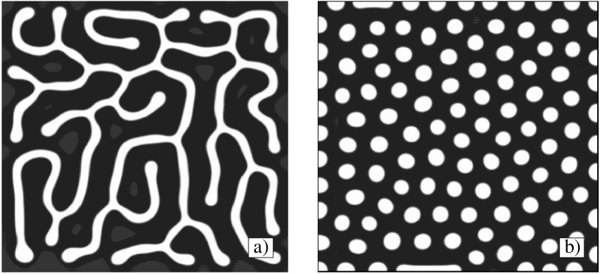
FIG. 2.: Two types of extended domain patterns: labyrinthine pattern (a) and multidomain pattern (b). Results of the numerical simulations of Eqs. (1) and (2) with $q=\theta^{3}-\theta-\eta$ and $Q=\theta+\eta-A$. The parameters used are: $\epsilon=0.05,\alpha=0.2,A=-0.4$. The system size is $20L\times 20L$. The time of the simulation is $500\tau_{\eta}$. For explanations of the initial conditions see the text.

Therefore, to the first power in $\epsilon$ and $K$ we may write Eq. (3) as follows:

$${\partial\theta\over\partial t}={\partial^{2}\theta\over\partial\rho^{2}}-K(\xi){\partial\theta\over\partial\rho}-q(\theta,\eta_{i}(\xi)).$$ (5)

The sign of $K$ is such that it is positive if the interface is convex into the low activator region. Notice that $\xi$ enters only as a parameter in this equation. For times $t\gg 1$ any solution of Eq. (5) connecting high and low values of the activator will become close to the solution in the form of a front propagating with the velocity $v$ in the direction perpendicular to the interface. For any given point $\xi$ one can then write

$$-v(\xi){d\theta\over dz}={d^{2}\theta\over dz^{2}}+K(\xi){d\theta\over dz}-q(\theta,\eta_{i}(\xi)),$$ (6)

where we introduced the self-similar variable $z=-\rho-vt$. The velocity is positive when it points out of the high activator value domain. The boundary conditions for this equation are:

$$\theta(+\infty)=\theta_{i1}(\xi),~{}~{}~{}\theta(-\infty)=\theta_{i3}(\xi),$$ (7)

where $\theta_{i1,3}$ are the minimal and the maximal roots of the equation

$$q(\theta_{i1,3}(\xi),\eta_{i}(\xi))=0$$ (8)

for any given $\xi$. The third solution $\theta_{i2}(\xi)$ of Eq. (8) which lies between $\theta_{i1}$ and $\theta_{i3}$ may be used to fix the position of the interface relative to $\theta(z)$ by requiring that $\theta=\theta_{i2}(\xi)$ on the interface. Thus, $v(\xi)$ represents the normal velocity of the pattern interface at a point $\xi$.

The velocity $v$ can be found by solving Eq. (6) with the abovementioned boundary conditions. The consistency condition which is obtained from Eq. (6) by multiplying it by $d\theta/dz$ and integrating over $z$ gives the following expression for the velocity in terms of $\theta(z)$:

$$v=-K-{\int_{\theta_{i1}}^{\theta_{i3}}q(\theta,\eta_{i})d\theta\over\int_{-\infty}^{+\infty}\left({d\theta\over dz}\right)^{2}dz}.$$ (9)

From this equation follows that the front velocity $v$ is of order 1. Notice that Eq. (6) is essentially an equation of motion of a particle in the potential

$$U_{\theta}=-\int q(\theta,\eta_{i})d\theta$$ (10)

with the friction proportional to $v+K$ with time $z$ [3, 4, 5]. In N systems $U_{\theta}$ is a double hump potential (for those values of $\eta_{i}$ for which it has only a single hump Eq. (6) has no solutions), so Eq. (6) has a unique solution which satisfies the boundary conditions in Eq. (7) for the given values of $\eta_{i}$ and $K$, which corresponds to the trajectory going from the top of one hump to the top of the other. Thus, the velocity of the interface is a single-valued function of the curvature and the value of $\eta$ at the interface.

FIG. 3.: The schematics of the system’s geometry (two dimensions). The thick solid line shows the interface. $\vec{e}_{\rho}$ and $\vec{e}_{\xi}$ are the local orthogonal basis of the curvilinear coordinate system $\rho,\xi$; $\rho$ indicates the distance from a given point to the interface, the dashed line indicates the surface $\rho=const$.

Far from the interfaces the activator varies on the characteristic length $\epsilon^{-1}$, so the Laplacian in Eq. (3) in that region can be dropped and Eq. (3) reads:

$${\partial\theta\over\partial t}=-q(\theta,\eta).$$ (11)

So, the relation between $\theta$ and $\eta$ far from the interfaces is local in space. Since $\eta$ varies on the length scales of order $\epsilon^{-1}$ or $K^{-1}$ and the velocity of the front is of order 1, the characteristic time of the variation of the interface velocity is also $\epsilon^{-1}\gg 1$ or $K^{-1}\gg 1$, what justifies the use of Eq. (6) for finding the distribution of the activator near the interfaces. The characteristic time of variation of the inhibitor field caused by the interface motion will also be $\epsilon^{-1}$ or $K^{-1}$ in the case $\alpha\gg\epsilon$ (fast inhibitor), or $\alpha^{-1}$, which is even greater than the previous in the case $\alpha\lesssim\epsilon$ (slow inhibitor), so the time derivative in Eq. (11) is less or of order $\epsilon$ and, therefore, can be neglected. Then, the values of $\theta$ and $\eta$ far from the interfaces are simply related by the equation of local coupling:

$$q(\theta,\eta)=0.$$ (12)

In view of Eq. (12), the inhibitor must satisfy the equation:

$$\alpha^{-1}{\partial\eta\over\partial t}=\epsilon^{-2}\Delta\eta-Q(\theta(\eta),\eta),$$ (13)

with the following boundary conditions at the interfaces (written in terms of the local curvilinear coordinates $\rho$ and $\xi$):

$$\eta(+0,\xi)=\eta(-0,\xi)=\eta_{i}(\xi).$$ (14)

The dependence $\theta(\eta)$ in Eq. (13) is the solution of Eq. (12). This dependence is multi-valued, so for the regions of high and low activator values one should take the branches connected with $\theta_{i3}$ and $\theta_{i1}$, respectively. Thus, we recovered the result obtained by Ohta, Mimura, and Kobayashi in Ref. [16] in the case of fast inhibitor as well. The term in the left-hand side of Eq. (13) is of order $\epsilon/\alpha$ which can be set equal to zero in the case of fast inhibitor.

Equation (13) is essentially nonlinear since it involves the inverse function of essentially nonlinear function $q(\theta,\eta)$, even if the Eq. (4) were linear. Moreover, the right-hand side of Eq. (13) becomes singular at the points $\theta_{0}$ and $\theta_{0}^{\prime}$ (see Fig. 1) where $q^{\prime}_{\theta}(\theta_{0},\eta_{0})=0$ and $q^{\prime}_{\theta}(\theta_{0}^{\prime},\eta_{0}^{\prime})=0$, respectively, since the function $\eta(\theta)$ becomes singular at these points. When the distribution of $\eta$ at a point $x_{0}$ reaches the values of $\eta_{0}$ or $\eta_{0}^{\prime}$, a sudden down-jump or up-jump (local breakdown), occurs at that point, respectively [3, 4, 5, 9, 15]. In terms of the free boundary problem this corresponds to the instantaneous creation of a new interface at the point $x_{0}$, which will start to evolve according to the equation of the interface motion. This is an important ingredient of the free boundary problem describing the dynamics of the pattern interface that should not be left out in solving this problem. Notice that local breakdown is responsible for the domain splitting in the one-dimensional N systems [3, 4, 5].

Equations (6) – (8) together with Eqs. (12) – (14) and the rule for dealing with the singularities of Eq. (13) discussed in the previous paragraph are the closed set of equations which defines completely the dynamics of any domain pattern in the system described by Eqs. (3) and (4) in the limit $\epsilon\rightarrow 0$ both in the case of slow and fast inhibitor. These equations were obtained with the accuracy to $\epsilon\ll 1$ and $K\ll 1$. Note that the presence of the curvature term in the equation of motion for the interface suggests only that the interface has to be sufficiently smooth, more exactly, it has to be smooth on the length scales of order 1. This, of course, does not mean that the interfaces are not allowed to intersect, fuse, or loose their connectivity in the course of their evolution. Self-replicating domains, which will be studied in the subsequent sections, are a good example of the latter. Also, a domain may disappear if it shrinks too much.

III non-local contour dynamics

As was shown in Ref. [9], when $\alpha\gg\epsilon$ static domain patterns may be stable only when their characteristic size is much smaller than the characteristic length of the inhibitor variation because of the stabilizing action of the interaction between the walls of the pattern. Typically, a pattern destabilizes when the characteristic distance between its walls (in the units of the previous Section) becomes of order $\epsilon^{-2/3}$ [9]. In this situation the velocity of the non-stationary pattern interface must be much smaller than one. Also, the value of the inhibitor must be close to the value of $\eta_{s}$ at which the velocity of the pattern wall is equal to zero in one dimension. According to Eq. (9) with $K=0$, the value of $\eta_{s}$ must satisfy

$$\int_{\theta_{s1}}^{\theta_{s3}}q(\theta,\eta_{s},A)d\theta=0,~{}~{}~{}~{}~{}q(\theta_{s1,3},\eta_{s},A)=0,$$ (15)

where $\theta_{s1}$ and $\theta_{s3}$ are some constants, which generally depend on $A$. This situation takes place when the bifurcation parameter $A$ is close to the values of $A_{b}$ or $A_{b}^{\prime}$ where the characteristic distance between the walls of the domains with high or low values of the activator becomes zero in the limit $\epsilon\rightarrow 0$.

For definiteness let us consider a single domain of high values of the activator. Then the value of the activator inside the domain will be close to $\theta_{s3}$, and to $\theta_{s1}$ outside. Let us introduce the new variables:

$$\tilde{\theta}=\theta-\theta_{s1},~{}~{}~{}~{}\tilde{\eta}=\eta-\eta_{s}$$ (16)

Equations (12) and (13) can then be linearized. In the case of fast inhibitor we will have:

$$q^{\prime}_{\theta}(\theta_{s1},\eta_{s})\tilde{\theta}+q^{\prime}_{\eta}(\theta_{s1},\eta_{s})\tilde{\eta}=0,$$ (17)

$$0=\epsilon^{-2}\Delta\tilde{\eta}-C\tilde{\eta}-aI(x)-Q(\theta_{s1},\eta_{s}),$$ (18)

where

$$C=Q^{\prime}_{\eta}(\theta_{s1},\eta_{s})-{Q^{\prime}_{\theta}(\theta_{s1},\eta_{s})q^{\prime}_{\eta}(\theta_{s1},\eta_{s})\over q^{\prime}_{\theta}(\theta_{s1},\eta_{s})},$$ (19)

$$a=Q(\theta_{s3},\eta_{s})-Q(\theta_{s1},\eta_{s}),$$ (20)

and $I(x)$ is the indicator function which is equal to 1 if $x$ is inside the domain and 0 outside. The value of $Q(\theta_{s1},\eta_{s})$ is small for $A$ close to $A_{b}$. Note that in writing Eq. (18) we neglected the piecewise-constant potential inside the domains which is present upon the linearization in the general case since one has to linearize Eq. (12) inside and outside of the domain separately. However, this is justified when the domain size is much smaller than the characteristic length of the inhibitor variation since the potential then is only a perturbation and can be neglected in the zeroth order.

Since the velocity of the front is small, it can also be linearized in $\tilde{\eta}$. This, however, extremely simplifies the problem since one no longer has to solve the non-linear eigenvalue problem in Eq. (6). Indeed, in the linear approximation in $\tilde{\eta}$ we can replace $\theta(z)$ in the denominator of Eq. (9) by the solution in the form of the static one-dimensional front and expand the numerator in $\tilde{\eta}$, so we immediately obtain for the velocity at a point $\xi$ on the interface:

$$v(\xi)=-K(\xi)-\tilde{\eta}_{i}(\xi)Z^{-1}\int_{\theta_{s1}}^{\theta_{s3}}q^{\prime}_{\eta}(\theta,\eta_{s})d\theta,$$ (21)

and

$$Z=\int_{\theta_{s1}}^{\theta_{s3}}\sqrt{2(U_{\theta}(\theta_{s1},\eta_{s})-U_{\theta}(\theta,\eta_{s}))}d\theta,$$ (22)

where $U_{\theta}$ is defined in Eq. (10).

The distribution of $\tilde{\eta}(x)$ at each moment in time and, therefore, the values of $\tilde{\eta}$ on the interface, which determine the interface velocity, can be found by solving Eq. (18) by means of the Green’s function:

$$\tilde{\eta}(x)=-{Q(\theta_{s1},\eta_{s})\over C}-a\int G(x-x^{\prime})I(x^{\prime})d^{d}x^{\prime}.$$ (23)

Specifically, in the infinite two-dimensional system

$$G(x-x^{\prime})=\frac{\epsilon^{2}}{2\pi}K_{0}(|x-x^{\prime}|\epsilon\sqrt{C}),$$ (24)

where $K_{0}$ is the modified Bessel function. Following the idea of Ref. [14], let us transform the integral in Eq. (23) in two dimensions into the contour integral along the interface. Using the defining equation for the Green’s function and the Gauss theorem, we find:

$$\tilde{\eta}(x)= -{Q(\theta_{s1},\eta_{s})\over C}$$ (26)

$$+\frac{a\epsilon}{2\pi\sqrt{C}}\oint\biggl{(}K_{1}(\epsilon r\sqrt{C})-\frac{1}{\epsilon r\sqrt{C}}\biggr{)}{\vec{r}\times d\vec{r}\over r},$$

where $\vec{r}$ is the vector from the point $x$ to $x^{\prime}$, where the point $x^{\prime}$ lies on the interface (see Fig. 3), and the integration is over the interface, $K_{1}$ is the modified Bessel function. In writing Eq. (26) it was taken into account that the surface integral obtained from Eq. (24) can as well be written in terms of the vector product involving the tangent vector $d\vec{r}$. The interface has to be oriented counterclockwise in order to get the sign right. If there is more than one domain in the system, one has to add up the contributions of each domain given by the integral in Eq. (26).

For a single domain of the size of order $\epsilon^{-2/3}$ one can expand the Bessel function in Eq. (26), so we obtain the following equation of motion for the interface:

$$v(\xi)=-K(\xi) -{BQ(\theta_{s1},\eta_{s})\over aCZ}$$ (28)

$$+\frac{B\epsilon^{2}}{4\pi Z}\oint(\ln(0.54\epsilon\sqrt{C})+\ln r)\vec{r}\times d\vec{r},$$

where

$$B=-(Q(\theta_{s3},\eta_{s})-Q(\theta_{s1},\eta_{s}))\int_{\theta_{s1}}^{\theta_{s3}}q^{\prime}_{\eta}(\theta,\eta_{s})d\theta,$$ (29)

and the point $x$ is now on the interface. If we introduce the renormalized coordinates, and time and introduce the new control parameter $\tilde{A}$:

$$\tilde{x}=x\epsilon^{2/3},~{}~{}\tilde{t}=t\epsilon^{4/3},~{}~{}\tilde{A}=-{BQ(\theta_{s1},\eta_{s})\epsilon^{-2/3}\over aCZ},$$ (30)

we will eliminate the $\epsilon$-dependence in Eq. (28) (except for the weak logarithmic dependence). Thus, we obtained the asymptotic equation of motion for a localized domain with the characteristic size much smaller than the characteristic size of the inhibitor variation. This equation was derived with the accuracy to $\epsilon^{2/3}$. Note that at this point all information about the specific nonlinearities of the system is contained only in a few numerical constants: $B$, $C$ and $Z$. These constants are all positive for the reaction-diffusion systems of the activator-inhibitor type [9]. Furthermore, they can be incorporated into the rescaled $\tilde{\epsilon}=\epsilon ZC^{3/2}/B$, provided that time and coordinate are also suitably rescaled. So, the dynamics of the localized domains in any two-dimensional N system not far from $A_{b}$ depends only on $\tilde{A}$ and $\tilde{\epsilon}$, the last dependence being logarythmically weak.

Equation (28) is also good for the description of several interacting domains if the distance between them is not much greater than $\epsilon^{-2/3}$. In order to study the interaction of domains separated by the distances of order $\epsilon^{-1}$ one has to use Eqs. (21) and (26).

Equation (28) contains a large logarithm which multiplies the integral $\oint\vec{r}\times d\vec{r}$ which up to a coefficient is the area of the domain. This means that with the logarithmic accuracy the area of the evolving domain has to be conserved. Also, the non-local term in Eq. (28) is an increasing function of $r$, so the parts of the interface which are close to each other attract, and the parts which are far from each other repel. Then the instability which appears for a radially-symmetric domain when its radius reaches certain value [9] cannot lead to the growth of a labyrinthine pattern, but rather will result in the domain splitting. The domains will then go apart and the process of splitting will repeat, until the systems becomes filled with the multidomain pattern. This mechanism of the instability development is qualitatively different from the one discussed in Ref. [14].

IV self-replicating domains in a concrete reaction-diffusion system

In this Section we will apply the results obtained above and show that the proposed mechanism of the instability development indeed takes place in a concrete reaction-diffusion system. To do this we will use the system which is described by Eqs. (3) and (4) with

$$q=\theta^{3}-\theta-\eta,$$ (31)

$$Q=\theta+\eta-A.$$ (32)

The nullclines of this system for $A=-0.6$ are shown in Fig. 1.

This system is particularly convenient because the dependences of its characteristic parameters on $A$ are especially simple. Also, the non-linear eigenvalue problem in Eq. (6) in this system admits exact solution. Simple calculation shows that:

$$\eta_{s}=0,~{}~{}~{}\theta_{s1}=-1,~{}~{}~{}\theta_{s3}=1,$$ (33)

and the coefficients involved in Eq. (28) are:

$$a=2,~{}~{}~{}B=4,~{}~{}~{}C=\frac{3}{2},~{}~{}~{}Z=\frac{2\sqrt{2}}{3}.$$ (34)

The value of $Q(\theta_{s1},\eta_{s})$ becomes zero at $A=A_{b}$ with $A_{b}=-1$. Also, the homogeneous state of the system $\theta_{h}=-|A|^{1/3},\eta_{h}=-|A|^{1/3}(1-|A|^{2/3})$ is stable for $A<A_{c}=-1/3\sqrt{3}$.

The solution of Eq. (6) can be sought in the form $\theta(z)=a\tanh bz+c$, where $a$, $b$, and $c$ are constants. As a result, the dependence of the front velocity on $\eta_{i}$ (with $K=0$) is implicitly given by the following equation:

$$v-\frac{2}{9}v^{3}=\frac{3}{\sqrt{2}}\eta_{i}.$$ (35)

The velocity $v$ satisfies $|v|<\sqrt{3/2}$, the maximum value being achieved at $\eta=\eta_{0}$, where $\eta_{0}=2/3\sqrt{3}$. Thus, for all values of $\eta$ for which Eq. (13) is not singular the dependence $v(\eta_{i})$ is single-valued.

Another special feature of this system is the fact that in it the piecewise-constant potential mentioned in Sec. III is identically zero, so Eqs. (21) and (26) also describe the dynamics of any complex pattern with the characteristic domain size much smaller than $\epsilon^{-1}$ for any values of $A$. These include the complex patterns forming in the late stages of the development of the transverse instabilities [9, 15]. In fact, the analog of Eq. (26), non-local both in space and time, may be obtained also in the case of arbitrary $\alpha$. This equation, together with Eq. (21), could be used to study the pulsations (breathing) of complex domain patterns in this system.

The direct numerical simulations of Eqs. (3) and (4) is a formidable task. The main difficulty here is the fact that for small $\epsilon$ there are two very different length scales, so the simulations require enormous amounts of computational power. Recently, it became possible to perform extensive numerical simulations of the system under consideration using massive parallelization on a supercomputer [15]. The authors were able to simulate the system of sufficiently large sizes with $\epsilon\simeq 0.05$. The values of $\epsilon\simeq 0.01$ are already very hard to simulate even on the very fast computer.

FIG. 4.: Destabilization of the circular domain. Results of the numerical simulation of Eq. (26) for the considered model with $\tilde{A}=20$ and $\epsilon=10^{-4}$. The box indicates the size of $30\times 30$. The length and time are measured in the rescaled units given by Eq. (28).

FIG. 5.: Self-replication of the domains. Results of the numerical simulation of Eq. (26) for the considered model with $\tilde{A}=30$ and $\epsilon=10^{-4}$. The box indicates the size of $30\times 30$. The length and time are measured in the rescaled units given by Eq. (28).

The main result of these simulations relevant to the present discussion is that as a result of the development of the transverse instability a localized domain transforms into a labyrinthine pattern, which is all connected if $A$ is not far from $A_{b}$. This effect takes place at $\epsilon>0.01$. For those values of $\epsilon$ domain splitting and self-replication was observed only when $\alpha\lesssim\epsilon$ [15]. We performed numerical simulations of this system for $\epsilon\leq 0.01$ and saw that a destabilizing localized domain actually splits into two. However, the simulation becomes excessively long at this point, so it is impossible to see if the forming domains will split in turn.

Equation (28), from the other hand, allows to study the interfacial dynamics for arbitrarily small $\epsilon$. We performed numerical simulations of Eq. (28) for the values of the parameters when a single localized domain becomes unstable with respect to transverse perturbations of its walls.

Figure 4 shows the evolution of the almost circular domain when its radius is close to the critical radius at which the domain loses stability with respect to the $m=2$ mode. Initially the domain elongates, but at some point the distance between the walls becomes so small that the domain splits into the three disconnected pieces. The resulting domains continue to grow until the larger domains split again into seven (not shown in the Figure), and the process goes on. Notice that in order for this process to take place, the value of $\epsilon$ has to be very small. As is seen from the numerical simulations of Eqs. (3) and (4), when $\epsilon$ is not very small the domain can elongate and transform into a stripe without splitting. This effect also takes place in the reaction-diffusion systems with the weak activator-inhibitor coupling [14].

Figure 5 shows the results of another simulation when the system is further away from the instability point. There the initial stage of the domain growth is similar to the one shown in Fig. 4. However, the walls in the center come closer to each other than in the previous case, so at some point the domain splits into two. The resulting domains continue to grow and split in turn. This process is essentially self-replication of the domains, as a result of which the system will become filled with the multidomain pattern.

We emphasize that unless the system is very close to the point $A=A_{b}$, the localized domains will always be unstable and, once excited, will transform into a multidomain pattern via self-replication even in the case of fast inhibitor, if $\epsilon$ is small enough. This is a completely universal result independent of any property of the system. In particular, this conclusion does not depend on whether the system is monostable or bistable. As was noted in the previous Section, the only nontrivial system-dependence is contained in the logarithmic term, and, therefore, this dependence is weak.

The results obtained for the system under consideration do not change in a wide range of $\epsilon$. When $\epsilon\gtrsim 0.01$, Eq. (28) seizes to be a good approximation for Eqs. (21) and (26). For extremely small $\epsilon$ ($\epsilon\lesssim 10^{-9}$) there exist a narrow region of the values of $\tilde{A}$ close to the critical value at which the disk transforms into a stable domain in the form of a dumbbell. When the value of $\tilde{A}$ is increased, the domain self-replication will occur even for such small values of $\epsilon$.

V conclusion

Thus, we have shown that in the case of fast inhibitor the transverse instability of the localized domains in the reaction-diffusion systems with N-shaped nullcline for the activator will always lead to domain splitting and formation of multidomain pattern rather than the formation of labyrinthine patterns, if $\epsilon$ is sufficiently small.

This effect was in fact observed in a quasi two-dimensional experiment with the current filaments forming in n-GaAs in the process of avalanche breakdown [17]. There the radially-symmetric current filaments destabilized and split as the current in the sample increased and the radius of a filament grew. At some critical value of current a filament split into two and the filaments that formed split in turn until their radii become sufficiently small. Non-symmetrically distorted or elongated filaments were not observed.

Hagberg and Meron suggested that splitting of domains is the consequence of the parity-breaking front transitions [nonequilibrium Ising-Bloch (NIB) transitions] associated with the variations of the curvature of the domain walls [13]. However, their arguments may apply only to the bistable reaction-diffusion systems in which the inhibitor is slow. We showed here that the splitting of domains in fact occurs in the systems with the fast inhibitor and is determined by the non-local interaction between different portions of the domain interface, regardless of whether the system is monostable or bistable, so as a rule the NIB transitions should not be responsible for domain splitting. It is clear that in the systems with the slow inhibitor domain splitting will occur even easier since the inhibitor will not be able to react on the motion of the walls of the domains locally not only in space, but also in time. This is also confirmed by the direct numerical simulations of Eqs. (1) and (2) [15].

Notice that the condition $\epsilon\ll 1$ itself is the necessary condition for the existence of the static domain patterns in the considered systems [3, 4, 5], so, in fact, the transition from a localized domain to the multidomain pattern consisting of disconnected localized domains filling up the space must be the major mechanism of the transverse instability development. Multidomain patterns were indeed observed in the chemical systems [10] and in the high-frequency gas discharge [18]. Nevertheless, numerical simulations and experimental observations also show that for small but finite $\epsilon$ localized domains may transform into extended labyrinthine patterns [10, 11, 12, 14, 15]. This does not seem to be the consequence of the finite width of the interface, but rather a peculiarity of the inhibitor dynamics. This effect can actually be controlled by varying the strength of interaction between the activator and the inhibitor [the constant $B$ in Eq. (28)]. Goldstein, Muraki, and Petrich analyzed the equation similar to Eqs. (21) and (26) in the case $B\sim\epsilon$ in the limit $\epsilon\rightarrow 0$ and found that the transverse instability leads to the formation of the connected labyrinthine pattern. This suggests that by changing $\epsilon$ or the coupling strength $B$ one could control whether the multidomain pattern or the labyrinthine pattern will form as a result of the domain instability.

It is important to note that the free boundary problem obtained from Eqs. (1) and (2) in the limit $\epsilon\ll 1$ contains considerably less information about the nonlinearities of the system than the initial partial differential equations problem. Moreover, according to Eq. (28), the behavior of any localized pattern not far from the points $A_{b}$ or $A_{b}^{\prime}$ is universal in the sense that the dynamics of the interface can be described by only a few renormalized parameters. This universality was discussed earlier in the context of the instabilities of the domain patterns [9]. This suggests that the free boundary formulation of the pattern dynamics might be a more advantageous starting point for dealing with the problems of domain pattern formation rather than the formulation in terms of reaction-diffusion equations.

The phenomenology of pattern formation similar to the one discussed in the present article is also observed in various equilibrium systems with competing interactions (see, for example, [8] and references therein). Notice that the reaction-diffusion system described by Eqs. (1) and (2) in the limit $\tau_{\eta}\rightarrow 0$ describes the kinetics of a system with competing interactions, if $q=f(\theta)-\eta$ and $Q=\eta+B\theta$, where $B$ is a constant and $f(\theta)$ is some cubic-like function [19, 20, 14]. These equations describe, for example, the kinetics of microphase separation of block copolymers [19, 21]. The universality of the results obtained above suggests that self-replication of domains must be a common feature of the systems with competing interactions in the case of repulsive long-range interactions of Coulombic type and strong separation of length scales.

The author is grateful to V. V. Osipov for valuable discussions.

REFERENCES

- [1] G. Nicolis and I. Prigogine, Self-organization in Non-Equilibrium Systems (Wiley Interscience, New York, 1977).
- [2] M. Cross and P. C. Hohenberg, Rev. Mod. Phys. 65, 851 (1993).
- [3] B. S. Kerner and V. V. Osipov, Autosolitons: a New Approach to Problems of Self-Organization and Turbulence (Kluwer, Dordrecht, 1994).
- [4] B. S. Kerner and V. V. Osipov, Sov. Phys. – Uspekhi 32, 101 (1989).
- [5] B. S. Kerner and V. V. Osipov, Sov. Phys. – Uspekhi 33, 679 (1990).
- [6] V. A. Vasiliev, Y. M. Romanovskii, D. S. Chernavskii, and V. G. Yakhno, Autowave Processes in Kinetic Systems: Spatial and Temporal Self-Organization in Physics, Chemistry, Biology, and Medicine (VEB Deutscher Verlag der Wissenschaften, Berlin, 1987).
- [7] J. D. Murray, Mathematical Biology (Springer-Verlag, Berlin, 1989).
- [8] M. Seul and D. Andelman, Science 267, 476 (1995).
- [9] C. B. Muratov and V. V. Osipov, Phys. Rev. E 53, 3101 (1996).
- [10] I. R. Epstein and I. Lengyel, Physica D 84, 1 (1995).
- [11] K. Lee and H. Swinney, Phys. Rev. E 51, 1899 (1995).
- [12] A. Hagberg and E. Meron, Phys. Rev. Lett. 72, 2494 (1994).
- [13] A. Hagberg and E. Meron, Chaos 4, 477 (1994).
- [14] R. E. Goldstein, D. J. Muraki, and D. M. Petrich, Phys. Rev. E 53, 3933 (1996).
- [15] C. B. Muratov and V. V. Osipov, (in preparation).
- [16] T. Ohta, M. Mimura, and R. Kobayashi, Physica D 34, 115 (1989).
- [17] K. M. Mayer, J. Parisi, and R. P. Huebner, Z. Phys. B – Cond. Matter 71, 171 (1988).
- [18] E. Ammelt, D. Schweng, and H.-G. Purwins, Phys. Lett. A 179, 348 (1993).
- [19] T. Ohta and K. Kawasaki, Macromolecules 19, 2621 (1986).
- [20] T. Ohta, A. Ito, and A. Tetsuka, Phys. Rev. A 42, 3225 (1990).
- [21] T. Ohta and A. Ito, Phys. Rev. E 52, 5250 (1995).