Weakly Nonlinear Theory of Pattern-Forming Systems with Spontaneously Broken Isotropy

Abstract

Quasi two-dimensional pattern forming systems with spontaneously broken isotropy represent a novel symmetry class, that is experimentally accessible in electroconvection of homeotropically aligned liquid crystals. We present a weakly nonlinear analysis leading to amplitude equations which couple the short-wavelength patterning mode with the Goldstone mode resulting from the broken isotropy. The new coefficients in these equations are calculated from the hydrodynamics. Simulations exhibit a new type of spatio-temporal chaos at onset. The results are compared with experiments.

Ac driven electroconvection (EC) in nematic liquid crystal (NLC) layers is one of the richest systems for the study of pattern forming phenomena [1, 2]. We consider the typical thin-layer geometry with the (slightly conducting) NLC sandwiched between glass plates coated with transparent electrodes. An ac voltage U is applied across the electrodes. By appropriate surface treatment of the glass plates the director ${{\bf\hat{n}}}$ (the preferred orientation of the NLC molecules) can be fixed at the boundaries. In particular the case of planar alignment (${{\bf\hat{n}}}$ in the plane of the layer) has been studied intensely. At onset one may then have normal rolls, where the wavevector is parallel to the undistorted director, or oblique ones.

The case of homeotropic surface anchoring (${{\bf\hat{n}}}$ aligned perpendicularly to the boundaries) where the system is isotropic in the plane of the layer (= $x$-$y$ plane) offers novel possibilities. Then, in the traditional EC materials with negative dielectric anisotropy, the voltage applied across the layer will first turn the director away from the layer normal (bend Freédericksz transition) leading to a quasi-planar director configuration (see e.g. [3]). The spontaneously chosen direction of the bend (i.e. direction of the projection of ${{\bf\hat{n}}}$ on the $x$-$y$ plane) will be denoted by ${\bf\hat{c}}={\bf\hat{c}}({\bf r},t)$ ($\,|{\bf\hat{c}}|\!=\!1\,$). Further increase of the voltage will eventually generate EC in close analogy to the planar case [4]; in fact nucleation to normal, oblique and traveling rolls has been observed [5]. The notable difference to the planar case is that the preferred axis (the in-plane director ${{\bf\hat{c}}}$) is degenerate and not fixed externally (neglecting unavoidable inhomogeneities and in the absence of a planar magnetic field). Then oblique rolls are not expected to lead to a stable pattern because they will in general exert a torque on ${{\bf\hat{c}}}$ which cannot be compensated. Even normal rolls, where a torque is absent because of symmetry, can be unstable because transverse modulations can be enhanced by the torque.

Here we will investigate the situation by setting up a novel weakly nonlinear description that incorporates the critical convection mode together with the Goldstone mode resulting from the spontaneous breaking of the $O(2)$ symmetry by the bend Freédericksz transition. The general form of the equations is derived from symmetry considerations. Analyzing the stability of rolls indicates that one may expect spatio-temporal chaos (STC) at onset under very general conditions. In fact this is probably the first experimentally accessible example of a nonrotating system with a direct transition to STC in a stationary (non-Hopf) bifurcation [5, 6]. The new coefficients of the equations are then calculated from the underlying standard hydrodynamic theory making quantitative comparison with experiments on MBBA (N-(p-methoxybenzylidene)-p-butylaniline) without adjustable parameters in principle possible. We end up by showing results of simulations.

First we consider the situation where the orientation of ${{\bf\hat{c}}}$ differs only by a small angle $\varphi$ from an overall direction that we choose as the $x$ axis (then ${\bf\hat{c}}=(cos\varphi,sin\varphi,0)\approx(1,\varphi,0)$). For simplicity we present the analysis for the normal-roll case, but it was done also for oblique rolls and some results will be given for that case. Let ${\bf q}_{c}=(q_{c},0)$, be the wavevector of the most unstable convection mode when $\varphi=0$. Near threshold the physical state can be written in the form

$${\bf V}({\bf r},z,t)= \bigl{(} {\bf V}^{(1)}(z,t)A({\bf r},t)e^{i{\bf q}_{c}\cdot{\bf r}}+\text{c.c.}\bigr{)}$$ (1)

$$+ {\bf V}_{G}(z,t)\varphi({\bf r},t)+h.o.t.,$$ (2)

where ${\bf V}$ is a formal vector consisting of the three components of the velocity, the director ${\bf\hat{n}}$, and the charge density. $A=\text{\it const.}$ and $\varphi=0$ yields the critical mode at the threshold $0=\varepsilon=(U^{2}-U_{c}^{2})/U_{c}^{2}$. The reduced description in terms of the modulation amplitudes $A$ and $\varphi$ has to respect the symmetries of the underlying hydrodynamic equations and the Freédericksz state. Thus we require invariance of the equations under translation (${\bf r}\to{\bf r}+{\bf r}_{0},\,A\to Ae^{-i{\bf q}_{c}\cdot{\bf r}_{0}}$), rotation ($\varphi\to\varphi+\delta,\,{\bf r}\to{\bf r}+\delta{\bf\hat{z}}\times{\bf r},\,\partial_{x}\to\partial_{x}-\delta\partial_{y},\,\partial_{y}\to\partial_{y}+\delta\partial_{x},\,A\to Ae^{i\delta{\bf\hat{z}}\times{\bf q}_{c}\cdot\vec{r}}$), three dimensional inversion ($x\to-x,\,y\to-y,\,A\to A^{*}$), reflection at the $x$ axis ($y\to-y,\,\varphi\to-\varphi$), and time-translation ($t\to t+t_{0}$). We consider the regime near onset ($\varepsilon,|A|\ll 1$) where slow spatial and temporal variations ($\partial_{x},\partial_{y},\partial_{t}\ll 1$) can be assumed. However, similar to [7] no specific scaling relations are assumed at this point.

By retaining only the leading terms allowed by symmetries the equations describing the evolution of $A$ and $\varphi$ can be determined up to prefactors:

$$\tau\partial_{t}A = \Big{[}\varepsilon+\xi_{xx}^{2}\partial_{x}^{2}+\xi_{yy}^{2}(\partial_{y}-iq_{c}\varphi)^{2}$$ (3)

$$- g|A|^{2}+i\beta_{y}\varphi_{,y}\;\Big{]}\,A,$$ (4)

$$\tilde{\gamma}_{1}\partial_{t}\varphi = K_{1}\partial_{y}^{2}\varphi+K_{3}\partial_{x}^{2}\varphi-\tilde{\chi}_{a}H^{2}\varphi$$ (5)

$$+ {\Gamma\over 4}(-iq_{c}A^{*}(\partial_{y}-iq_{c}\varphi)A+\text{c.c.}).$$ (6)

In (3) and in similar equations the derivative operators $\partial_{x}$, $\partial_{y}$ operate on $A$ only, while $\varphi_{,y}$ is the derivative of $\varphi$ in the $y$ direction. All coefficients are real and we will assume all but $\beta_{y},\Gamma$ to be positive. The coefficients $\beta_{y}$ and $\Gamma$ describe the novel effects. The last expression in Eq. (5) describes the torque exerted by the roll pattern on ${\bf\hat{c}}$. An additional term $-\tilde{\chi}_{a}H^{2}\varphi$ is included in Eq. (5) to allow a continuous transition from the rotationally invariant case to the case of fixed ${{\bf\hat{c}}}$, as for planarly aligned cells. Physically $H$ corresponds to a stabilizing magnetic field parallel to the $x$-axis. In the special case $\beta_{y}=-\xi_{yy}^{2}q_{c}$ the angle $\varphi$ would play the role of a gauge field and Eq. (3) could be derived from a potential. If also $\Gamma>0$, both equations can be derived from a Lyapunov functional. However, in our non-equilibrium system there is no reason to assume existence of a potential. For MBBA we find $\Gamma<0$, which implies a “repulsive torque” between the direction of the local wavevector and ${\bf\hat{c}}$. Then at $H=0$ all ordered roll solutions are in fact unstable (see below).

For $H=0$ Eqs. (3,5) become uniform in $\varepsilon$ when the scaling $\partial_{x},\partial_{y},A,\varphi\sim\varepsilon^{1/2}$ and $\partial_{t}\sim\varepsilon$ is adopted. This is a major difference to similarly looking coupled amplitude equations describing mean-flow effects in isotropic Rayleigh-Bénard convection [7, 8, 9]. Since $\varphi$ is also scaled, this is not applicable to Eqs. (22,24) below because there $\varphi$ is $2\pi$ periodic.

After rescaling (3,5) one arrives at the normal form

$$\check{\tau}\partial_{t}\check{A} = \Big{[}1+\partial_{x}^{2}+(\partial_{y}-i\check{\varphi})^{2}$$ (7)

$$- |\check{A}|^{2}+i\check{\beta}_{y}\check{\varphi}_{,y}\;\Big{]}\,\check{A},$$ (8)

$$\partial_{t}\check{\varphi} = \partial_{y}^{2}\check{\varphi}+\check{K}_{3}\partial_{x}^{2}\check{\varphi}-\varepsilon^{-1}\check{H}^{2}\check{\varphi}$$ (9)

$$+ \check{\Gamma}\;(-i\check{A}^{*}(\partial_{y}-i\check{\varphi})\check{A}+\text{c.c.}),$$ (10)

where $A=(\varepsilon/g)^{1/2}\check{A}$, $x=\xi_{xx}\varepsilon^{-1/2}\check{x}$, $y=\xi_{yy}\varepsilon^{-1/2}\check{y}$, $\varphi=\varepsilon^{1/2}\check{\varphi}/(\xi_{yy}q_{c})$, $t=\tilde{\gamma}_{1}\xi_{yy}^{2}\check{t}/(\varepsilon K_{1})$, $\check{\beta}_{y}=\beta_{y}/(\xi_{yy}^{2}q_{c})$, $\check{K}_{3}=K_{3}\xi_{yy}^{2}/(K_{1}\xi_{xx}^{2})$, $\check{H}^{2}=\chi_{a}\xi_{yy}^{2}H^{2}/K_{1}$, $\check{\Gamma}=q_{c}^{2}\xi_{yy}^{2}\Gamma/(4gK_{1})$, $\check{\tau}=K_{1}\tau/(\gamma_{1}\xi_{yy}^{2})$. The caret $\check{\text{\ }}$ has been suppressed on the variables $x$, $y$, $t$ in Eqs. (7,9).

The stationary, uniform solutions of these equations are $\check{A}=\check{A}_{0}e^{i(Qx+Py)}$, $\check{\varphi}=\check{\varphi}_{0}=2\check{\Gamma}\check{A}_{0}^{2}P/(\check{H}^{2}/\varepsilon+2\check{\Gamma}\check{A}_{0}^{2})$, $A_{0}^{2}=1-(P-\check{\varphi}_{0})^{2}-Q^{2}$. We now present the main results of the stability analysis of these roll solutions. For $\check{\Gamma}<0$ and $H=0$ rolls are always unstable at onset, and one expects a (direct) transition to spatio-temporal chaos. For $\check{H}\neq 0$ and $\check{\beta}_{y}<0$ one has a kind of Eckhaus instability associated with a finite angle between the director and the local wavevector of the rolls, whereas for $\check{\beta}_{y}>0$ an instability induced by director modulations via the $\check{\beta}_{y}$-term in (7) is dominating.

Perturbations can in general be cast in the following form:

$$\delta\check{A} = (A^{+}e^{st+i(k_{x}x+k_{y}y)}+A^{-}e^{s^{*}t-i(k_{x}x+k_{y}y)})e^{i(Qx+Py)},$$ (11)

$$\delta\check{\varphi} = (\tilde{\varphi}e^{st+i(k_{x}x+k_{y}y)}+\text{c.c.}).$$ (12)

The case $\check{\varphi}_{0}=0=P$ is particularly simple. Then the constant-amplitude solutions are stable if $\check{H}^{2}/\varepsilon+2\check{\Gamma}(1-Q^{2})>0$, $\check{H}^{2}/\varepsilon+2\check{\Gamma}(1-Q^{2})(1+\check{\beta}_{y})>0$ and $Q^{2}<1/3$ (Eckhaus criterion). For $\check{H}=0$ stable rolls require $\check{\Gamma}>0$, $1+\check{\beta}_{y}>0$ and $Q^{2}<1/3$. Otherwise one has stability if $P\check{\Gamma}/\check{\varphi}_{0}>0$, $\check{\beta}_{y}\check{\varphi}_{0}/P>-1$ and $\det M_{ij}>0$, where

$$M_{xx} = 1-(P-\check{\varphi}_{0})^{2}(1+2\check{\varphi}_{0}/P)-3Q^{2},$$ (13)

$$M_{xy} = M_{yx}=(P-\check{\varphi}_{0})Q((1-\check{\beta}_{y})\check{\varphi}_{0}/P-2),$$ (14)

$$M_{yy} = (1+\check{\beta}_{y}\check{\varphi}_{0}/P)(1-3(P-\check{\varphi}_{0})^{2}-Q^{2}).$$ (15)

The direction of $(k_{x},k_{y})_{\text{crit}}$ at the marginal point $\det M_{ij}=0$ is given by the null space of $M_{ij}$.

At the generalized Eckhaus boundary $(P-\check{\varphi}_{0})^{2}+Q^{2}=1/3$ known for planarly aligned EC [2], $\det M_{ij}\sim-(\check{\varphi}_{0}/P)^{2}$ is already negative. Thus, as expected, the additional degree of freedom $\varphi$ leads to a destabilization of the system.

Expanding for small $P$ and $Q$ we find the uniform solution to be stable for $\check{H}^{2}>\check{H}^{2}_{\text{crit}}$ where

$${\check{H}^{2}_{\text{crit}}\over\varepsilon}=-2\check{\Gamma}\check{A}_{0}^{2}\left(1+3^{1/2}|P|+3P^{2}+{\text{h.o.t.}}\right)$$ (16)

if $\beta_{y}<0$ and

$${\check{H}^{2}_{\text{crit}}\over\varepsilon}=-2\check{\Gamma}\check{A}_{0}^{2}\left(1+\check{\beta}_{y}+{(1+\check{\beta}_{y})^{4}\over\check{\beta}_{y}^{3}}P^{2}Q^{2}+{\text{h.o.t.}}\right)$$ (17)

if $\beta_{y}>0$. Since in the latter case the r.h.s. is dominated by the quadratic dependence of $\check{A}_{0}^{2}$ on $P$, $Q$, small but finite $P$, $Q$ are more stable then $P,Q=0$.

We expect that an experimental verification of the stability analysis is possible. Note that the value of $P$ can be adjusted by turning the magnetic field with respect to the probe after a stable roll pattern has been established.

The analogous equations for the amplitudes $A_{1}$, $A_{2}$ of oblique rolls (zig and zag) have additional terms and the expression for the torque on ${\bf\hat{c}}$ acquires the form ${\Gamma q_{c}p_{c}}(|A_{1}|^{2}-|A_{2}|^{2})/2$. If the crossed-roll solution $|A_{1}|=|A_{2}|$ is preferred over simple rolls (e.g. $A_{1}\neq 0$, $A_{2}=0$) the situation is presumably analogous to that of normal rolls (no torque on the director for the unmodulated solution). In the opposite case (as for MBBA) the resulting equations have no nontrivial time-independent roll solution. In that case $\varepsilon$ cannot be scaled out completely and one gets different scaling ranges.

Next we describe the calculation of the coupling coefficients $\beta_{y}$ and $\Gamma$ from the standard hydrodynamic equations for NLCs [10, 11]. The other coefficients are obtained following standard procedures (see e.g. [11, 12]). As usual the set of equations is decomposed into a sum of operators operating on the state vectors ${\bf V}={\bf V}({\bf r},z,t)$. Each operator is linear in each of its arguments:

$$0=O({\bf V})=-B\partial_{t}{\bf V}+L{\bf V}+N_{2}({\bf V}|{\bf V})+\dots$$ (18)

The operator $O({\bf V})$ depends on $\varepsilon$ in two ways: by the explicit action of the electric field and the field dependence of the Freédericksz state, which is the basic state in this formalism.

Two components can be distinguished in the kernel of $L$: the convective mode ${\bf V}^{(1)}$ at wavevectors ${\bf q}=\pm{\bf q}_{c}$ and the Goldstone mode ${\bf V}_{G}$ at ${\bf q}=0$ [4] normalized such that it corresponds to $\delta n_{y}=\partial{{\bf\hat{c}}}/\partial\varphi|_{\varphi=0}$. Near onset these two modes govern the dynamics described in Eqs. (3,5). We will also need the linear eigenmodes ${\bf V}^{(1)}(p)$, ${\bf V}_{G}(p)$ of (18) into which ${\bf V}^{(1)}$ and ${\bf V}_{G}$ develop for transverse modulations, i.e. at ${\bf q}=\pm(q_{c},p)$ and $\pm(0,p)$ respectively. The coefficients are obtained in some analogy to the treatment of mean-flow effects [7, 8, 9] and of the concentration field in binary fluids [13].

Let $\langle{\bf V}_{1},{\bf V}_{2}\rangle$ be a scalar product and ${{\bf V}^{(1)}}^{+}(p)$ and ${{\bf V}_{G}}^{+}$ be the adjoint eigenvectors of $L$ corresponding to ${\bf V}^{(1)}(p)$ and ${\bf V}_{G}$. The coefficient $\beta_{y}$ in Eq. (3) turns out to be

$$\beta_{y}\!=\! -\langle{{\bf V}^{(1)}}^{+},(\partial_{\varepsilon}L){\bf V}^{(1)}\rangle^{-1}{d\over dp}\biggl{\langle}{{\bf V}^{(1)}}^{+}(p),$$ (20)

$$\left(N_{2}({\bf V}^{(1)}|{\bf V}_{G}(p))+N_{2}({\bf V}_{G}(p)|{\bf V}^{(1)})\right)\biggr{\rangle}\biggr{|}_{p=0\atop\varepsilon=0}.$$

The coefficient of the hydrodynamic angular momentum in (5) is

$${\Gamma q_{c}\over 2}=C{d\over dp}{\langle{{\bf V}_{G}}^{+},N_{2}({\bf V}(p)|{\bf V}(p))\rangle}\Big{|}_{p=0},$$ (21)

where $C$ is chosen such, that $\tilde{\gamma}_{1}=1$.

In order to explore the attractor in the roll-unstable case and to compare the long-time dynamics with experiments the assumption that $\varphi$ be small must be relaxed (at least at $H=0$). One in fact only needs the condition, that the local wavevector differs little from a (local) critical wavevector $q_{c}{{\bf\hat{c}}}$. Formally this can be achieved by reintroducing the fast variation ($\tilde{A}=Ae^{i{\bf q}_{c}\cdot{\bf r}}$) and rewriting derivatives and the magnetic torque in rotation-invariant form (we write ${\bf\hat{c}}_{\perp}={\bf\hat{z}}\times{\bf\hat{c}}$):

$$\tau\partial_{t}\tilde{A} = \Big{[}\varepsilon+\xi_{xx}^{2}({\bf\hat{c}}\cdot\partial_{{\bf r}}-iq_{c})^{2}+\xi_{yy}^{2}({\bf\hat{c}}_{\perp}\cdot\partial_{{\bf r}})^{2}$$ (22)

$$- g|\tilde{A}|^{2}+i\beta_{y}{\bf\hat{c}}_{\perp}\cdot\nabla\varphi\Big{]}\,\tilde{A},$$ (23)

$$\gamma_{1}\partial_{t}\varphi = K_{3}{\bf\hat{c}}_{\perp}\cdot\nabla^{2}{{\bf\hat{c}}}+(K_{1}-K_{3}){\bf\hat{c}}_{\perp}\cdot\nabla(\nabla\cdot{{\bf\hat{c}}})$$ (24)

$$+ \chi_{a}({\bf\hat{c}}\cdot{\bf H})({\bf\hat{c}}_{\perp}\cdot{\bf H})+{\Gamma\over 4}(-iq_{c}\tilde{A}^{*}({\bf\hat{c}}_{\perp}\cdot\partial_{{\bf r}})\tilde{A}\!+\!\text{c.c.}).$$ (25)

These equations have been used for numerical simulations.

In Fig. 1 we compare snapshots of $\psi=\tilde{A}+c.c.$ from our simulations (left side) with experiments (right side) from [5, 6] ($\varepsilon=0.02$, $H=0$). Material parameters as in [4] were used to calculate the coefficients of (22,24). For normal rolls (upper pair), at the experimental driving frequency $\omega\tau_{0}=1.75$ ($\tau_{0}=\epsilon_{0}\epsilon_{\bot}/~{}\sigma_{\bot}$ is the charge relaxation time) the calculated coefficients are: $\tau=0.0292$, $q_{c}=2.71$, $\xi_{xx}^{2}=0.434$, $\xi_{yy}^{2}=0.225$, $\beta_{y}=-0.60$, $K_{1}=1.01$, $K_{3}=1.28$, $g=4.37$, $\Gamma=-12.8$, $\chi_{a}=1$. (We measure length in units of $d/\pi$ with $d$ the thickness of the fluid layer, time in director relaxation times $\tau_{d}=\gamma_{1}d^{2}/k_{11}\pi^{2}$ and magnetic fields in Freédericksz fields $H_{f}^{2}=k_{11}\pi^{2}/\chi_{a}d^{2}$.) For oblique rolls (at $\omega\tau_{0}=0.73$, lower pair) we proceeded analogously. In order to obtain a good fit to the wavelength the thickness $d=28.5\,{\rm\mu m}$ was used instead of the nominal value $d=20\,{\rm\mu m}$ given in [14] ($d$ was not measured directly). This only rescales length.

The patterns in experiments and simulations look very similar. Though in the normal roll regime some defects appear, the rolls are locally aligned along some main direction. In the simulations we find the pattern to change on a time scale $t_{c}/\epsilon=0.8$ ($t_{c}$ is defined by $\left<\psi(\vec{r},t-t_{0})\psi({\bf r},t_{0})\right>_{{\bf r},t_{0}}\sim\exp(-|t|/t_{c})$) while the experimental state appeared to be time independent. Presumably some pinning of the pattern in the experiments is responsible for this disagreement. The oblique roll regime is dominated by a superposition of zig and zag. Again the preferred axis changes only over large distances. A persistent time dependence was observed in simulations ($t_{0}/\epsilon=0.5$) and experiments. Unfortunately the experiments are still preliminary so far. A systematic experimental investigation is under way [15].

Equations (7,9) represent normal-form equations for quasi-2D pattern-forming systems with a novel kind of symmetry, and should thus be of general interest. Other realizations might be found in convection instabilities in smectic-C liquid crystals, where one has a ${\bf\hat{c}}$-director from the beginning on, and in Rayleigh-Bénard convection of homeotropically aligned NLCs with an additional electric field. In this case the fields that drive the Freédericksz transition and the convection instability, respectively, can be varied independently, which should allow to access a large parameter range of Eqs. (7,9).

For $H=0$ and $\Gamma<0$ Eqs. (22,24) describe STC at onset. There is some analogy to a recent investigation of a 1d model for seismic waves, where a spontaneous symmetry breaking is also important [16]. Other examples of STC at onset are the Küppers-Lortz instability (in rotating Rayleigh-Bénard convection [17, 18]) and systems undergoing a Hopf bifurcation. Here one has the Benjamin-Feir destabilization mechanism (see e.g. [19] and as a recent example [20]) and the so-called dispersive chaos where a quantitative description by a simple Ginzburg-Landau equation should be possible [21]. The origin of chaotic behavior is of course very different in the various systems and their detailed comparison appears fruitful. Work on the characterization of the complex spatio-temporal states is in progress, with particular emphasis on the transition to order under the influence of the stabilizing magnetic field.

For ordinary stationary bifurcations (and Hopf bifurcations in the Benjamin-Feir stable range) the onset of STC is presumably always at finite $\varepsilon$ (possibly quite small), at least as long as effects from lateral boundaries play no role. Examples are the usual case of EC with planar alignment [22], besides our system in the presence of a stabilizing magnet field.

We wish to thank A. Buka and H. Richter for discussions and providing us with unpublished materials. This work was supported by Deutsche Forschungsgemeinschaft (Graduierten-Kolleg “Nichtlineare Spektroskopie und Dynamik”) and Volkswagen Stiftung.

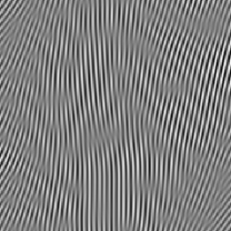
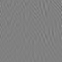
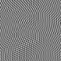
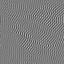
FIG. 1.: Simulations of Eqs. (22,24) (left) vs. experiment [23] (right) for normal (top) and oblique (bottom) rolls (see text).

REFERENCES

- [1] I. Rehberg, B. L. Winkler, and M. de la Torre, Adv. Solid State Physics 29, 35 (1989).
- [2] L. Kramer and W. Pesch, Annu. Rev. Fluid Mech. 27, 515 (1995).
- [3] P.G. de Gennes and J. Prost, The Physics of Liquid Crystals, Claredon Press, Oxford, 1993.
- [4] A. Hertrich, W. Decker, W. Pesch, and L. Kramer, J. Phys. France II 2, 1915 (1992).
- [5] H. Richter, A.Buka, and I.Rehberg, Phys.Rev. E 51, 5886 (1995); H. Richter, N. Klöpper, A. Hertrich, and A. Buka, Europhys. Lett. 30, 37 (1995).
- [6] K. Hayashi, Y. Hidaka and S. Kai, Proc. of the 1st Tohwa Univ. Stat. Phys. Meeting (1995); M. I. Tribelsky, K. Hayashi, Y. Hidaka, S. Kai, Proc. of the 1st Tohwa Univ. Stat. Phys. Meeting (1995).
- [7] A. J. Bernoff, Euro. J. Appl. Math. 5, 267 (1994).
- [8] E. D. Siggia and A. Zippelius, Phys.Rev.Lett. 47, 835 (1981).
- [9] W. Decker and W. Pesch, J.Phys.II France 4, 493 (1994).
- [10] S. Chandrasekhar, Liquid Crystals (University Press, Cambridge, 1992).
- [11] E. Bodenschatz, W. Zimmermann, and L. Kramer, J. Phys.(Paris) 49, 1875 (1988).
- [12] P. Manneville, Dissipative Structures and Weak Turbulence (Academic Press, New York, 1990).
- [13] H. Riecke, Phys. Rev. Lett. 68, 301 (1992).
- [14] H. Richter, Ph.D. thesis, Universität Bayreuth, 1995.
- [15] P. Toth, A. Buka, privat communication.
- [16] M. I. Tribelsky, and K. Tsuboi, Phys. Rev. Lett. 76, 1631 (1996); M. I. Tribelsky, Int. J. Bif. Chaos, in press.
- [17] G. Küppers and D. Lortz, J. Fluid Mech. 35, 609 (1969).
- [18] Y. Hu, R. E. Ecke, and G. Ahlers, Phys. Rev. Lett 74, 5040 (1995).
- [19] M. C. Cross, and P. C. Hohenberg, Rev. Mod. Phys. 65, 851 (1993).
- [20] M. Dennin, D. Cannell, and G. Ahlers, Mol. Cryst. Liq. Cryst. 261, 977/337 (1995); M. Dennin, M. Treiber, L. Kramer, G. Ahlers and D. Cannell, Phys.Rev.Lett. 76, 319 (1996).
- [21] P. Kolodner, S. Slimani, N. Aubry, and R. Lima, Physica D 85, 165 (1995).
- [22] M. Kaiser and W. Pesch, Phys. Rev. E 48, 4510 (1993); M. Kaiser, W. Pesch, and E. Bodenschatz, Physica D 59, 320 (1992).
- [23] H. Richter, A.Buka, and I.Rehberg (unpublished).