A Simple model for Faraday Waves

Abstract

We show that the linear-stability analysis of the birth of Faraday waves on the surface of a fluid is simplified considerably when the fluid container is driven by a triangle waveform rather than by a sine wave. The calculation is simple enough to use in an undergraduate course on fluid dynamics or nonlinear dynamics. It is also an attractive starting point for a nonlinear analysis.

I Introduction

Parametrically excited surface waves, or Faraday waves, are generated when a container of fluid is vertically vibrated. Above an acceleration threshold, waves appear on the fluid surface. The waves vibrate at half the driving frequency, a feature associated with the parametric resonance that is responsible for pumping energy into the surface-wave modes.

In most “Faraday experiments,” the container is driven sinusoidally. That is, its vertical position may be described by $x(t)=(x_{pp}/2)\cos\omega t$, and its acceleration by $a(t)=-\omega^{2}(x_{pp}/2)\cos\omega t$. In this paper, we explore the consequences of driving the container with a triangle-wave forcing. Although the difference between the two waveforms matters little physically, we shall show that it simplifies the analysis remarkably.

There are two broad motivations for our study. First, although the theory of hydrodynamic stability occupies an important conceptual place in current courses in hydrodynamics, standard examples such as thermal convection (Rayleigh-Bénard Convection, or RBC) and shear flow between rotating concentric cylinders (Taylor-Vortex Flow, or TVF) are too complicated to present in standard undergraduate courses. Textbooks for such courses (e.g., [1]) usually limit themselves to heuristic arguments. By contrast, our analysis is simple enough to present in a single class to third- or fourth-year students. (The calculation’s difficulty is equivalent to solving the Kronig-Penney model for energy bands in a one-dimensional solid. This example is commonly presented in undergraduate solid-state-physics courses.)

A second motivation comes from the increasingly prominent role that the Faraday experiment occupies as an example of a non-equilibrium pattern-forming system. Most of the work on pattern formation done to date has focused on convection (RBC) and shear flow (TVF) [2]. However, a recent series of papers has established a number of advantages for the Faraday experiment [3, 4, 5, 6, 7, 8, 9]. Very large cells ($>10^{2}$ wavelengths wide) may be created, and the basic (“fast”) time scale can be very short ($t_{0}\lesssim 10^{-2}$ sec.) The short time scale is particularly important because the dynamics of pattern-forming instabilities is often slow. Current work looks at features that occur on time scales of $10^{4}t_{0}$ to $10^{5}t_{0}$. Convection, by contrast, usually has $t_{0}\approx 1$ sec., or slower.

As we shall show below, our variant of the Faraday experiment clarifies our understanding of the instability itself. The analysis separates into two pieces: one is the derivation of the surface-wave dispersion relation (Section III); the other is the description of how parametric pumping injects energy into the fluid (Section II). By choosing triangle-wave forcing, we greatly simplify the latter piece. We hope that this will ultimately allow the nonlinear analysis (particularly of high-viscosity fluids) to be pursued further than it has been hitherto. For this reason, we make no restriction on the fluid viscosity; the only approximation made is in linearizing the Navier-Stokes equations.

The body of this paper is organized as follows: In Section II, we study the related problem of the Mathieu equation with delta-function forcing. Solving this problem turns out to be mathematically equivalent to solving for the acceleration thresholds of Faraday waves. In Section III, we apply this analysis to the Faraday experiment with triangle-wave forcing. In Section IV, we consider a simple extension, driving by an asymmetric triangle wave, which models the recent “two-frequency” experiments that have attracted much attention [6]. Section V contains a brief conclusion.

II The Mathieu Equation with Delta-Function Forcing

An infinitely extended continuous system such as a fluid can be thought of as containing a continuum number of modes. To linear order, the modes are independent and the system’s behavior can be determined from the study of each mode separately. Nonlinear effects imply mode coupling. In this section, we examine the effects of parametric forcing on a single mode. In Section III, we apply the results derived here to the continuum of modes present in the Faraday experiment.

There are two ways to pump energy into an oscillator. The first is by direct forcing, where the prototypical equation is

$$\ddot{x}+2\gamma\dot{x}+\omega_{0}^{2}x=f(t),$$ (1)

where $f(t)$ is the driving force and is often chosen to be $f\cos\omega t$. For small damping $\gamma$, a directly forced oscillator has a resonant response (of amplitude $\approx f/\omega_{0}\gamma$) at $\omega\approx\omega_{0}$.

The second way to pump energy into an oscillator is by parametric forcing, whose prototypical equation is the (damped) Mathieu equation:

$$\ddot{x}+2\gamma\dot{x}+\omega_{0}^{2}[1+f(t)]x=0.$$ (2)

When $f(t)$ is sinuosoidal, there is an infinite series of resonances centered on $\omega=2\omega_{0}$, $\omega_{0}$, $(2/3)\omega_{0}$, $\omega/2$, $...,(2/n)\omega_{0}$, for integer $n$. The strongest of these resonances is the first ($n=1$), and a response at half the driving frequency is good evidence that a system is being driven parametrically. Below, we shall find it convenient to rephrase the resonance conditions in terms of periods: $\Delta t=(n/2)T$, where $\omega=2\pi/\Delta t$ and $\omega_{0}=2\pi/T$.

Although $f(t)$ may be sinusoidal, the solutions $x(t)$ are not. Let $f(t)=f\cos 2\omega_{0}t$ and assume $x(t)=x_{0}\cos\omega_{0}t.$ The term $f(t)x(t)$ in Eq. (2) is proportional to $\cos\omega_{0}t\cos 2\omega_{0}t$ and can be rewritten as $(1/2)(\cos\omega_{0}t+\cos 3\omega_{0}t)$, implying that $x(t)$ has a $3\omega_{0}t$ component. Adding this to $x(t)$ generates a $5\omega_{0}t$ term, and so on. Eq. (2) must in general be solved numerically. For special choices of $f(t)$, however, Eq. (2) may be solved analytically. The simplest case is $f(t)$ equal to a sum of delta functions [10]. A slightly more complicated case, $f(t)$ equal to a square wave, was discussed in these pages some years ago [11]. In Section III, we show that analyzing a fluid container driven by a triangle wave is equivalent to studying the Mathieu equation driven by a series of equal-amplitude delta functions, with alternating signs. (See Fig. 1b.) Here, we review the analysis of [10] for the particular case of delta-function forcing with equal and then with alternating signs.

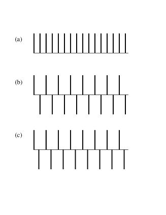
FIG. 1.: Driving function $f(t)$. (a) Periodic train of delta functions of equal signs. (b) Periodic train of delta functions of alternating signs, derived from a symmetric triangle wave. (c) Periodic train of delta functions of alternating sign, derived from an asymmetric triangle wave.

A Mathieu equation driven by a periodic series of delta functions

In units where time, damping rate, and forcing are all scaled by $\omega_{0}$, we wish to solve

$$\ddot{x}+2\gamma\dot{x}+[1+\varepsilon\sum_{n}\delta(t-n\Delta t)]x=0.$$ (3)

The forcing function is shown in Fig. 1a. In between delta-function “kicks,” the system is just a free, damped oscillator. Let $x_{n}(t)$ be the solution valid between the kicks at $n\Delta t$ and $(n+1)\Delta t$. One finds

$$x_{n}(t)=A_{n}e^{\psi(t-t_{n})}+\rm{c.c.}$$ (4)

with $\psi=-\gamma\pm i\omega_{0}^{\prime}$ and $\omega_{0}^{\prime}=\sqrt{1-\gamma^{2}}$. The kick imposes two conditions linking $x_{n}$ and $x_{n+1}$:

$\bullet$ $x$ is continuous.

$\bullet$ the velocity $\dot{x}$ jumps discontinuously. This condition can be derived by integrating Eq. (3) over a small interval of time centered on $t_{n+1}$.

The conditions may be expressed as:

$$x_{n+1}(t_{n+1}) = x_{n}(t_{n+1})$$ (6)

$$\dot{x}_{n+1}(t_{n+1}) - \dot{x}_{n}(t_{n+1})+\varepsilon x_{n}(t_{n+1})=0.$$ (7)

Imposing the continuity and velocity-jump conditions allows one to relate $A_{n+1}$ to $A_{n}$:

$$\left(\begin{array}[]{c}A_{n+1}^{r}\\ A_{n+1}^{i}\end{array}\right)=e^{-\gamma\Delta t}\left(\begin{array}[]{cc}C&-S\\ S+\alpha C&C-\alpha S\end{array}\right)\left(\begin{array}[]{c}A_{n}^{r}\\ A_{n}^{i}\end{array}\right),$$ (8)

where $A_{n}^{r}$ and $A_{n}^{i}$ are the real and imaginary parts of $A_{n}$, respectively, $C=\cos\omega_{0}^{\prime}\Delta t$, $S=\sin\omega_{0}^{\prime}\Delta t$, and $\alpha=\varepsilon/\omega_{0}^{\prime}$ is the scaled forcing amplitude.

Eqs. (4) and (8) constitute a solution to Eq. (3). Given initial conditions $A_{0}$, we can find $x(t)$ by first iterating the map $e^{-\gamma\Delta t}M$ to find the proper $A_{n}$. Here, $M$ is the $2\times 2$ matrix in Eq. (8). Then use Eq. (4) to find $x(t)$.

Eq. (8) can also be used to find the acceleration threshold for resonant response. Parametric resonance differs from ordinary resonance in that it is a true instability. If $\varepsilon$ is below a threshold $\varepsilon_{c}$, $x(t)\to 0$ at long times. For $\varepsilon>\varepsilon_{c}$, $x(t)$ grows without bounds. (Adding a nonlinear term in $x$ to Eq. (3) will limit the oscillator’s amplitude. In practice, nonlinearities are always present in the physical situation being modeled.) Our goal now is to find $\varepsilon_{c}({\Delta t})$.

The key observation is that the long-time amplitude of the motion $x(t)$ is controlled by the eigenvalues of the matrix $M$: if their magnitude is greater than $e^{\gamma\Delta t}$, the motion’s amplitude will grow each period. If the magnitude of both eigenvalues is less than $e^{\gamma\Delta t}$, damping will reduce the motion each cycle and the system will tend towards $x(t)=0$. Loosely speaking, $M$ accounts for the energy pumped into the system during each period $\Delta t$, while $e^{-\gamma\Delta t}$ represents the energy lost during $\Delta t$.

The matrix $M$ has unit determinant. If we write $M$ in the general form $\left(\begin{array}[]{cc}A&B\\ C&D\end{array}\right)$ the eigenvalues are given by $\lambda_{1,2}=x\pm\sqrt{x^{2}-1}$ where $x=(A+D)/2=(1/2)$Tr$M$. Instability arises when both eigenvalues are real and the magnitude of the largest exceeds $e^{\gamma\Delta t}$. Simple algebraic manipulations then give for the threshold condition

$$x=\pm\cosh\gamma\Delta t$$ (9)

In the present case, the matrix elements are $A=\cos\omega_{0}^{\prime}\Delta t$ and $D=\cos\omega_{0}^{\prime}\Delta t-{\varepsilon\over\omega_{0}^{\prime}}\sin{\omega_{0}^{\prime}\Delta t}$. Inserting these into the threshold condition Eq. (9), we find

$$\varepsilon_{c}({\Delta t})=2\omega_{0}^{\prime}\left({\cos\omega_{0}^{\prime}\Delta t\pm\cosh\gamma\Delta t\over{\sin\omega_{0}^{\prime}\Delta t}}\right)$$ (10)

This threshold condition is plotted in Fig. 2a for different choices of the damping $\gamma$. The curves generated by choosing the plus sign are centered on $\Delta t=(n/2)T,n=1,3,5,...$ and are known as subharmonic “tongues,” while the curves generated by choosing the minus sign are centered on $\Delta t=mT$, $m=1,2,3,...$ and are known as harmonic tongues. These curves are qualitatively similar to those of the Mathieu Eq. with sinusoidal forcing [12, 13].

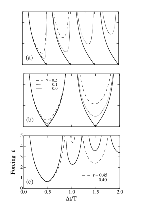
FIG. 2.: Resonance tongues for the Mathieu eq. driven by a periodic sequence of delta functions, for $\gamma$ = 0.0, 0.1, and 0.2. (a) Delta functions of equal sign. (b) Delta functions of alternating signs. (c) Delta functions derived from an asymmetric triangle wave, for $\gamma=0.2$ and different values of $r\equiv\Delta t_{2}/\Delta t$. For $r=0.5$, the tongues are the same as the dashed lines in (b). Note how the harmonic tongues are more prominent as the asymmetry is increased ($r\to 0$).

B Mathieu equation driven by a sequence of delta functions of alternating sign

In our version of the Faraday experiment, the container’s vertical position $x(t)$ is a triangle wave. Taking two time derivatives of $x(t)$, we see that the acceleration $a(t)$ is a periodic sequence of delta functions of equal magnitude but alternating sign. For this reason, we generalize the analysis of section II A to a driving term of the form

$$\varepsilon\left\{\sum_{n}\left[\delta(t-n\Delta t)-\delta[t-(n+1/2)\Delta t]\right]\right\}x(t)$$ (11)

Let $x_{n}(t)$ be the solution valid over $(n\Delta t)<t<[(n+1/2)\Delta t]$ and let $x_{n+1/2}(t)$ be the solution valid over $[(n+1/2)\Delta t]<t<[(n+1)\Delta t]$. Except for the kicks at $(n\Delta t)$ and $[(n+1/2)\Delta t]$, the oscillator is free and we have

$$x_{n}(t) = A_{n}e^{\psi(t-t_{n})}+{\rm c.c.}$$ (13)

$$x_{n+1/2}(t) = A_{n+1/2}e^{\psi(t-t_{n+1/2})}+{\rm c.c.}$$ (14)

Applying the continuity and jump conditions at $(n\Delta t)$ and $[(n+1/2)\Delta t]$, we find

$$\left(\begin{array}[]{c}A_{n+1}^{r}\\ A_{n+1}^{i}\end{array}\right) = e^{-\gamma\Delta t/2}\left(\begin{array}[]{cc}c&-s\\ s+\alpha c&c-\alpha s\end{array}\right)\left(\begin{array}[]{c}A_{n+1/2}^{r}\\ A_{n+1/2}^{i}\end{array}\right)$$ (22)

$$\vspace{0.25in}\left(\begin{array}[]{c}A_{n+1/2}^{r}\\ A_{n+1/2}^{i}\end{array}\right) = e^{-\gamma\Delta t/2}\left(\begin{array}[]{cc}c&-s\\ s-\alpha c&c+\alpha s\end{array}\right)\left(\begin{array}[]{c}A_{n}^{r}\\ A_{n}^{i}\end{array}\right),$$ (29)

where $c\equiv\cos{\omega_{0}^{\prime}\Delta t/2}$ and $s\equiv\sin{\omega_{0}^{\prime}\Delta t/2}$. Combining these, we can write $A_{n+1}=e^{-\gamma\Delta t}M_{2}M_{1}A_{n}\equiv e^{-\gamma\Delta t}MA_{n}$. Since det$M=$ (det $M_{1}$)(det $M_{2})=1$, we have the same threshold condition, $x=\pm\cosh\gamma\Delta t$, leading to

$$\varepsilon_{c}(\Delta t)=2\omega_{0}^{\prime}\sqrt{{\cos\omega_{0}^{\prime}\Delta t\pm\cosh\gamma\Delta t}\over 1-\cos\omega_{0}^{\prime}\Delta t}$$ (30)

The resonance tongues are shown in Fig. 2b. There are only subharmonic tongues, a feature that turns out to be special to the use of our particular driving function Eq. (11).

To understand more intuitively why there is resonance for the subharmonic case but not for the harmonic case, consider the two time series shown in Fig. 3. Fig 3a shows a time series for $(\Delta t=T/2$, $\omega=2\omega_{0}$), where $T=2\pi/\omega_{0}$ is the natural period of the oscillator. Fig. 3b shows the case $(\Delta t=T$, $\omega=\omega_{0})$. The delta-function impulses are indicated by up and down triangles on each curve while the force vector for each kick is indicated by an arrow above or below the triangle. Because the delta functions are multiplied by the coordinate $x$, the sign of the velocity increment depends on the position of the particle relative to the origin. In the subharmonic case, the impulse always increases the speed of the motion. In the harmonic case, the up triangles decrease the speed, while the down triangles add to it. Because the overall motion is damped, it is clear that the net effect of the kicks is to decrease the energy of the system. One can understand this better by considering the matrices $M_{1}$ and $M_{2}$ in the limit of zero damping (harmonic case). The cos$\omega_{0}^{\prime}\Delta t/2$ and sin$\omega_{0}^{\prime}\Delta t/2$ terms are then $-1$ and $0$, respectively, and the product $M_{2}M_{1}$ is just the identity matrix, independent of the value of the forcing $\alpha$. Thus, no energy is added to the system even as it is forced arbitrarily hard. (One kick adds energy while the next one removes it.) When damping is added, as in Fig. 3b, the system is always stable about $x=0$. The harmonic case differs from the harmonic case of sinusoidal driving, where there is still a resonance because the forcing is distributed over the whole period of the oscillator.

Note that when $\gamma>0$, higher order tongues have higher thresholds than the $\omega=2\omega_{0}$ tongue. The bottom of this first tongue defines an overall threshold that represents the global-minimum amplitude $\varepsilon^{*}$ required to excite oscillations. We can find $\varepsilon^{*}(\gamma,\omega_{0})$ by differentiating Eq. (30) for $\varepsilon(\Delta t)$. This yields $\cot\omega_{0}^{\prime}\Delta t/2={\gamma/\omega_{0}^{\prime}}\tanh\gamma\Delta t/2$ for $\Delta t^{*}(\gamma,\omega_{0})$. This transcendental equation can be solved numerically or perturbatively for small $\gamma/\omega_{0}$, which gives $\Delta t\approx\pi/\omega_{0}[1-(1/2)(\gamma/\omega_{0})^{2}]$ and $\omega=2\omega_{0}[1+(1/2)(\gamma/\omega_{0})^{2}]$. To lowest order in $\gamma/\omega_{0}$, the resonance conditions are just the zero-viscosity ones: $\Delta t=\pi/\omega_{0}$ and $\omega=2\omega_{0}$. At this order, the overall forcing threshold is given by $\varepsilon^{*}=\pi\gamma$.

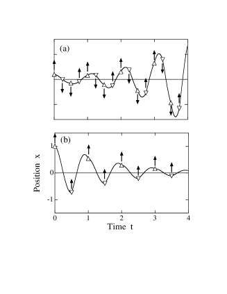
FIG. 3.: Time series $x(t)$ for the Mathieu eq. driven by a periodic sequence of delta functions of alternating signs. In both time series, the damping $\gamma=0.1$ and the forcing $\varepsilon=0.7$. The triangles show where the forcing is applied. They point up for positive delta functions and down for negative delta functions. The arrows above the triangles indicate the direction of the force vector for each kick. Because the delta function forcing term multiplies the coordinate $x$, the sign of the force vector opposes that of the delta function for $x<0$. Time is in units of the undamped-oscillator period ($2\pi$). (a) Subharmonic case (b) Harmonic case.

III Faraday Waves with Triangle-Wave Forcing

In this section, we shall apply the above results to the linear-stability analysis of the flat surface of a viscous fluid held in a laterally infinite container of fluid of infinite depth. (The finite-depth case is straightforward, but the algebra is longer [15].) Already in 1883, Rayleigh had suggested that the instability studied fifty years earlier by Faraday might be due to the phenomenon of parametric resonance, and he wrote down and explored the properties of Eq. (2) independently of Mathieu [14]. Seventy years later, Benjamin and Ursell [12] showed that the normal modes of the linearized, inviscid Navier Stokes equations each obeyed a Mathieu equation. In the Benjamin-Ursell calculation, the effects of damping must be added perturbatively (using $\gamma=2\nu k^{2}/\omega\ll 1$ as the bulk dissipation coefficient, where $\nu=\eta/\rho$ is the kinematic viscosity and $k$ the magnitude of the wavenumber of the disturbance). Recently (1994) Kumar and Tuckerman performed a complete linear analysis that is valid for all viscosities [13]. Since the analysis for arbitrary viscosity is only slightly more complicated than that for small viscosity, we present the more general result.

We begin by deriving the equations of motion, following Kumar and Tuckerman. The Navier-Stokes equations of motion for the fluid layer are

$$[\partial_{t}+\vec{U}\cdot\vec{\nabla}]\vec{U} = -{1\over\rho}\vec{\nabla}P+\nu\nabla^{2}\vec{U}-g(t)\hat{z}$$ (32)

$$\vec{\nabla}\cdot\vec{U} = 0.$$ (33)

Here, $\vec{U}(x,y,z,t)$ is the fluid velocity field in the lab frame of reference and $P(x,y,z,t)$ is the pressure field. There is a simple solution, corresponding to a fluid at rest in its own frame of reference: $\vec{U}=0$ and $P(t)=-\rho g(t)z$.

Linearizing about the at-rest solution, we find for the perturbing fields $\vec{u}$ and $p$

$$\partial_{t}\vec{u} = -{1\over\rho}\vec{\nabla}p+\nu\nabla^{2}\vec{u}$$ (35)

$$\vec{\nabla}\cdot\vec{u} = 0.$$ (36)

(In the new frame of reference, gravity does not appear in the bulk equations of motion. It will resurface in the boundary conditions.) Applying the operator ($\hat{z}\cdot\vec{\nabla}\times\vec{\nabla}\times$) and using the incompressibility condition $\vec{\nabla}\cdot\vec{u}=0$, we eliminate the pressure and obtain

$$(\partial_{t}-\nu\nabla^{2})\nabla^{2}u=0,$$ (37)

where $u\equiv u_{z}(x,y,z,t)$ is the $z$-component of the velocity field.

At the bottom of the cell, no-slip boundary conditions imply that $\vec{u}=0$. Using the incompressibility condition, we rewrite this as

$$u=\partial_{z}u=0.$$ (38)

At the air-fluid interface, there are three conditions. The first is a kinematic one that relates the fluid velocity to the position of the interface:

$$[\partial_{t}+\vec{u}\cdot\vec{\nabla}]\zeta=u|_{z=\zeta},$$ (39)

where $\zeta(x,y,t)$ is the location of the interface. To linearize, we drop the $\vec{u}\cdot\vec{\nabla}$ term and evaluate the right-hand side at $z=0$, giving $\partial_{t}\zeta=u|_{z=0}$.

The second condition asserts that there are no tangential stresses at the interface. Since the interface normal is just $\hat{z}$ to first order, one has that $\pi_{xz}=\pi_{yz}=0$ at $z=0$, where the stress tensor $\pi$ is defined as

$$\pi_{ij}=-P\,\delta_{ij}+\eta\,(\partial_{i}u_{j}+\partial_{j}u_{i})=\left[-p+\rho g(t)z\right]\,\delta_{ij}+\eta\,(\partial_{i}u_{j}+\partial_{j}u_{i}),$$ (40)

with $i$ and $j$ ranging over $x$, $y$, and $z$, and where $\eta$ is the ordinary fluid viscosity. Taking the horizontal divergence of Eq. (40), we have

$$\nabla^{2}_{H}u+\partial_{z}(\vec{\nabla}_{H}\cdot\vec{u_{H}})=(\nabla^{2}_{H}-\partial_{zz})u=0,$$ (41)

where ${\vec{u}_{H}}$ is the horizontal velocity field at $z=0$ and the incompressibility condition was used to write the last identity.

The third condition relates the normal stress to the Laplace pressure caused by surface tension acting on a curved interface:

$$\pi_{zz}=\gamma\kappa\approx-\gamma\nabla_{H}^{2}\zeta,$$ (42)

where $\kappa$ is the mean curvature of the interface and the second term comes from writing the curvature to first-order in $\zeta$. We have, at $z=0$,

$$p(\zeta)=2\eta\left(\partial_{z}u\right)+\rho g(t)\zeta+\gamma\nabla_{H}^{2}\zeta.$$ (43)

Taking the horizontal divergence of the Navier–Stokes equation, one can obtain a second relation involving the pressure field and use this to rewrite Eq. (43) in terms of $u$ and $\zeta$ alone:

$$(\partial_{t}-\nu\nabla^{2})(\partial_{z}u)=2\nu\nabla_{H}^{2}(\partial_{z}u)+g(t)\nabla_{H}^{2}\zeta-{\gamma\over\rho}\nabla_{H}^{4}\zeta.$$ (44)

Because the horizontal eigenfunctions of a laterally infinite container are $e^{\pm i\vec{k}\cdot\vec{r}}$, we can replace $\nabla_{H}^{2}$ by $-k^{2}$, and $\nabla^{2}$ by $(\partial_{zz}-k^{2})$. We then have the following linearized equations of motion for $u$:

 

$$\left[\partial_{t}-\nu(\partial_{zz}-k^{2})\right](\partial_{zz}-k^{2})u = 0$$ (46)

$$u = \partial_{z}u=0\hskip 72.26999ptz=-\infty$$ (47)

$$(\partial_{zz}+k^{2})u\left|{}_{z=0}\right. = 0\hskip 108.405ptz=0$$ (48)

$$\left[\partial_{t}-\nu(\partial_{zz}-k^{2})+2\nu k^{2}\right](\partial_{z}u)|_{z=0} = -\left[g[1-f(t)]-{\gamma\over\rho}k^{3}\right]k^{2}\zeta$$ (49)

$$\partial_{t}\zeta = u|_{z=0}$$ (50)

As with the Mathieu eq., one can easily solve the unforced equations between kicks, where surface waves propagate and are damped by viscosity. Let $u_{n}(z,t)$ be the $z$-component of the velocity valid for $(n\Delta t)<t<(n+(1/2)\Delta t)$. Let $\zeta_{n}(t)$ be the amplitude of surface displacement over the same time period. From Eqs. (III), we find

$$u_{n}(z,t) = e^{\psi(t-t_{n})}u_{n}(z)+{\rm c.c.}\hskip 72.26999ptu_{n}(z)=a_{n}e^{\kappa z}+b_{n}e^{kz}$$ (52)

$$\zeta_{n}(t) = \zeta_{n}e^{\psi(t-t_{n})}+{\rm c.c.}\hskip 90.3375pt\kappa^{2}=k^{2}+\psi/\nu$$ (53)

Eqs. (III) give $a_{n}=-2\nu k^{2}\zeta_{n}$ and $b_{n}=(2\nu k^{2}+\psi)\zeta_{n}$. The normal-stress condition (Eq. 49) gives the dispersion relation $\psi(k)$ for the surface waves:

$$\psi=-2\nu k^{2}\pm i\omega_{0}\sqrt{1-{4\nu^{2}k^{3}\kappa\over{\omega_{0}^{2}}}},$$ (54)

where $\omega_{0}^{2}\equiv gk+(\gamma/\rho)k^{3}$. Note that this expression for $\psi$ resembles the one found for the Mathieu equation. (See Eq. 4 and the line following.) The laterally infinite container supports a continuum of modes indexed by the 2D wavenumber $\vec{k}=(k_{x},k_{y})$. A mode of wavenumber $k$ has a damping coefficient $\gamma\approx 2\nu k^{2}$. Damping gives a (second-order) decrease in the frequency, so that $\omega_{0}^{\prime}=\omega_{0}\sqrt{1-{4\nu^{2}k^{3}\kappa\over\omega_{0}^{2}}}.$ One complication, relevant only for higher viscosities, is that Eq. (54) is an implicit equation for $\psi$, since $\kappa=\kappa(\psi)$. One can write (and solve) an explicit, fourth-order equation for $\psi(k)$, but not much insight is gained. The important point is that $\psi(k)$ is the dispersion relation for free surface waves propagating on a deep, viscous fluid. Such dispersion relations have been catalogued for a variety of physical situations (small or large depth, small or large viscosity, viscoelastic effects, surfactant layers on the surface, etc.). One can look up or calculate the appropriate $\psi(k)$ for each physical situation one wishes to study. The dispersion relation is completely independent of the way the waves are excited (parametric or direct forcing). For now, we leave $\psi(k)$ as arbitrary.

The next step is to derive the matrices relating the complex amplitudes $\zeta_{n+1}$ to $\zeta_{n+1/2}$ to $\zeta_{n}$. At $(n+1/2)\Delta t$, continuity of $\zeta$ yields Re$(\zeta_{n+1/2})=$ Re$(\zeta_{n}e^{\psi\Delta t/2})$. The velocity-jump condition is derived by integrating the normal-stress condition Eq. (49) over a small interval of time centered on $(n+1/2)\Delta t$. We find

 

$$(\partial_{z}u_{n+1/2}|_{z=0})(t_{n+1/2})-(\partial_{z}u_{n}|_{z=0})(t_{n+1/2})={4x_{pp}k^{2}\over{\Delta t}}(-1)\left[\zeta_{n}e^{\psi\Delta t/2}+{\rm c.c.}\right]$$ (55)

where

$$\left(\partial_{z}u_{n+1/2}\right)(t_{n+1/2})=\kappa a_{n+1/2}+kb_{n+1/2}+\rm{c.c.}=[2\nu k^{2}(k-\kappa)+\psi k]\zeta_{n+1/2}+\rm{c.c.}$$ (56)

Inserting this into Eq. (55), we find

$${\rm Im}\zeta_{n+1/2}={\rm Im}\zeta_{n}e^{\psi\Delta t/2}+{4x_{pp}k\over{\Delta t}}{1\over{({\rm Im}\psi-2\nu k{\rm Im}\kappa})}{\rm Re}\zeta_{n}e^{\psi\Delta t/2}$$ (57)

 

Define now $\psi\equiv-\gamma+i\omega_{0}^{\prime}$ and $\kappa=\kappa_{r}+i\kappa_{i}$. Then $\zeta_{n+1}=e^{-\gamma\Delta t/2}M_{2}\zeta_{n+1/2}$ and $\zeta_{n+1/2}=e^{-\gamma\Delta t/2}M_{1}\zeta_{n}$. Here, the matrices $M_{1}$ and $M_{2}$ have exactly the same form as before, except that now $\alpha=4x_{pp}k/[(\Delta t)(\omega_{0}^{\prime}-2\nu k\kappa_{i})]$. The tongues then are given by $2\alpha({\Delta t})=\sqrt{{\cos\omega_{0}^{\prime}\Delta t\pm\cosh\gamma\Delta t}\over 1-\cos\omega_{0}^{\prime}\Delta t}$. One difference is that in a laterally infinite container, all modes $\vec{k}$ are available. Thus, whatever the driving frequency $\omega$ (or whatever the $\Delta t$), the response of all modes must be considered. This implies that the overall threshold $\varepsilon^{*}$ discussed above is the relevant concept. Since the $\omega=2\omega_{0}$ tongue is in general the easiest to excite, one expects waves at just half the driving frequency.

For small damping $(\sigma\equiv 4\nu k^{2}/\omega\ll 1)$, one has $\gamma\approx 2\nu k^{2}$, $\kappa=k$, $\omega_{0}^{\prime}\approx\omega\approx 2\omega_{0}$, giving a threshold of

$$a_{pp}=\left({\pi^{2}\over 2}\right)\nu k\omega,$$ (58)

which is slightly higher than the corresponding condition for sine-wave forcing [5], $a_{pp}=4\nu k^{2}\omega.$

IV Driving by an Asymmetric Triangle Wave

Recently, Edwards and Fauve [6] have explored the effects of exciting Faraday waves with a driving signal that is the sum of two sine waves of rationally related frequency. They showed that for fixed frequency ratio (5:4 in their original work), the relative amplitude and phase of the two sine waves could be considered as independent control parameters. Varying these new parameters dramatically affects the pattern-formation selection. For example, they produced hexagons and quasi-periodic patterns (“quasi-patterns”) under conditions where single-frequency forcing would lead to a stripe pattern.

Here, we look at a simple model of two-frequency forcing, an asymmetric triangle-wave forcing (Fig. 1c). This waveform has the crucial feature that it is asymmetric under time reversal, $f(t)\neq f(\Delta t-t)$, in contrast with the “single-frequency” driving waveform (Fig. 1b). As Edwards and Fauve have argued, time-reversal invariance of $f(t)$ implies that the nonlinear amplitude equations for the parametrically excited waves must be invariant under $A\to-A$; however, this symmetry is removed for asymmetric $f(t)$.

In the delta-function model, asymmetric triangle-wave forcing is easily solved by replacing the $\Delta t/2$ in the matrices $M_{1}$ and $M_{2}$ (Cf. Eqs. 11) with $\Delta t_{1}$ and $\Delta t_{2}$, where $\Delta t_{1}+\Delta t_{2}=\Delta t$. The tongue boundaries for the Mathieu Eq. are then given by

$$\varepsilon_{c}({\Delta t})=\sqrt{2}\omega_{0}^{\prime}\sqrt{{\cos\omega_{0}^{\prime}\Delta t\pm\cosh\gamma\Delta t}\over{\sin\omega_{0}^{\prime}\Delta t_{1}\sin\omega_{0}^{\prime}\Delta t_{2}}}.$$ (59)

The tongues are plotted for several choices of $\Delta t_{1}$ and $\Delta t_{2}$ in Fig. 2c. Note the reappearance of the harmonic tongues for $\Delta t_{1}\neq\Delta t_{2}$. In this simple model, there is no analog of the “bicritical point” discussed by Edwards and Fauve, where two different wavenumbers go unstable simultaneously. Nonetheless, the symmetry argument given above suggests that asymmetric-triangle-wave forcing will alter the nonlinear pattern selection in much the same way as two frequencies do.

V Conclusion

In this paper, we have shown how the linear-stability analysis of Faraday waves is greatly simplified for triangle-wave forcing. Our analysis is simple enough to include in an undergraduate hydrodynamics course. One could also combine the analysis with a simple experiment to make a good senior thesis project. References [6] and [15] give careful discussions of the required experimental apparatus [18].

Our calculation may also serve as the starting point for a more extensive nonlinear analysis. To date, nonlinear amplitude equations for Faraday waves have been derived only in the limit of small damping $\sigma\ll 1$ [16, 17]; however, many interesting phenomena are seen when $\sigma\approx 0.4$ to $0.7$ [9]. With delta-function driving, the effects of the parametric pumping are straightforward, even in the nonlinear regime. The hard part of the calculation becomes the determination of nonlinear terms in the dispersion relation for surface waves. However, this is a problem that has received much attention over the years, and a number of results are available [19].

REFERENCES

- [1] D. J. Tritton, Physical Fluid Dynamics, 2nd. ed. (Oxford Univ. Press, Oxford, 1988), Cf. Ch. 17.
- [2] M. C. Cross and P. C. Hohenberg, “Pattern formation outside of equilibrium,” Rev. Mod. Phys. 65 851-1112 (1993).
- [3] A. B. Ezersky, M. I. Rabinovich, V. P. Reutov, and I. M. Starobinets, “Spatiotemporal chaos in the parametric excitation of a capillary ripple,” Sov. Phys. JETP 64 1228-1236 (1986).
- [4] B. Christiansen, P. Alstrøm, and M. T. Levinsen, “Ordered capillary-wave states: quasicrystals, hexagons, and radial waves, Phys. Rev. Lett. 68 2157-2160 (1992).
- [5] S. Fauve, K. Kumar, C. Laroche, D. Beysens, and Y. Garrabos, “Parametric instability of a liquid-vapor interface close to the critical point Phys. Rev. Lett. 68 3160-3163 (1992).
- [6] W. S. Edwards and S. Fauve, “Patterns and quasi-patterns in the Faraday experiment,” J. Fluid Mech. 278 123-148 (1994).
- [7] E. Bosch and W. van de Water, “Spatiotemporal intermittency in the Faraday experiment,” Phys. Rev. Lett. 70 3420-3423 (1993).
- [8] B. J. Gluckman, C. B. Arnold, and J. P. Gollub, “Statistical studies of chaotic wave patterns,” Phys. Rev. E 51 1128-1147 (1995).
- [9] L. Daudet, V. Ego, S. Manneville, and J. Bechhoefer, “Secondary instabilities of surface waves on viscous fluids in the Faraday instability,” Europhys. Lett. 32 313-318 (1995).
- [10] C. S. Hsu, “Impulsive parametric excitation: theory,” J. Appl. Mech. 39, 551-558 (1972).
- [11] E. D. Yorke, “Square-wave model for a pendulum with oscillating suspension,” Am. J. Phys. 46, 285-288 (1978).
- [12] T. B. Benjamin and F. Ursell, “The stability of the plane free surface of a liquid in vertical periodic motion,” Proc. R. Soc. Lond. A 225 505-515 (1954).
- [13] K. Kumar K. L. S. Tuckerman, “Parametric instability of the interface between two fluids,” J. Fluid Mech. 279 49-68 (1994); Cf. J. Beyer and R. Friedrich, “Faraday instability: linear analysis for viscous fluids,” Phys. Rev. E 51, 1162-1168 (1995).
- [14] Lord Rayleigh, “On maintained vibrations,” Phil. Mag. 15 229-235 (1883). “On the crispations of fluid resting upon a vibrating support,” Phil. Mag. 16 50-58 (1883). Reprinted in Scientific Papers by Lord Rayleigh, Vol. II, pp. 188-193 and pp. 212-219. Dover, 1964.
- [15] J. Bechhoefer, V. Ego, S. Manneville, and B. Johnson, “An experimental study of the onset of parametrically pumped surface waves in viscous fluids,” J. Fluid Mech. 288 325-350 (1995).
- [16] S. T. Milner, “Square patterns and secondary instabilities in driven capillary waves,” J. Fluid Mech. 225 81-100 (1991).
- [17] W. Zhang, “Pattern formation in weakly damped parametric surface waves,” Ph. D. Thesis, Florida State Univ., (1994).
- [18] The electromagnetic shaker tables that are usually used to generate Faraday waves will not give an accurate output if a function generator is used to create the triangle wave. Because of the inductance of the vibration coils, the different frequency components of the input waveform will have different phase shifts and the result will be far from a triangle wave. A straightforward work-around is to use the feedback system of [6], which requires a modest amount of programming. Alternatively, one could design a vibrator specifically for triangle waveforms.
- [19] L. Debnath, Nonlinear Water Waves, (Academic Press, San Diego, 1994), pp. 62-66.