Non-Monotonic Dispersion of Surface Waves in Magnetic Fluids

Abstract

The dispersion relation of surface waves of a magnetic fluid in a magnetic field is studied experimentally. We verify the theoretically predicted existence of a non-monotonic dispersion relation. In particular, we demonstrate the existence of two different wave numbers occuring at the same frequency in an annular geometry.

I Introduction

The science of magnetic fluids is a multidisciplinary field, which encompasses physics, chemistry, mathematics, engineering and medical sciences [1]. One of its interesting features is the spontaneous formation of patterns under the influence of an external magnetic field [2]. If a static magnetic field is applied normal to the surface, the so called normal field- or Rosensweig-instability will occur at a critical value of the magnetisation leading to a deformation of the surface. Due to theoretical considerations [2], the advent of this pattern forming instability is accompanied by a non-monotonic dispersion relation. This interesting behaviour is not a unique feature of magnetic fluids, however. Similar behaviour is expected for polarizable fluids under the influence of a normal electric field [3]. Both theories apply for an inviscous fluid in an infinite layer. Although experimental studies of externally induced surface waves have been published [4, 5], an experimental verification of the non-monotonic dispersion of surface waves is missing so far. We thus present an experimental attempt to verify the existence of a non-monotonic dispersion relation for surface waves in a magnetic fluid.

II Experimental Setup and Procedure

The experimental setup is shown in Fig. 1. We use the commercially available magnetic fluid EMG 909 (Ferrofluidics) with the following properties: density $\rho=1020$ kgm^-3, surface tension $\sigma=2.65\cdot 10^{-2}$ kgs^-2, initial magnetic permeability $\mu=1.8$, magnetic saturation $M_{S}=1.6\cdot 10^{4}$ Am^-1, viscosity $\eta=6\cdot 10^{-3}$ Nsm^-2.

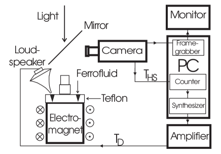
FIG. 1.: Experimental setup.

The fluid is filled into a V-shaped [6] cylindrical teflon channel of 6 cm diameter as indicated in Fig. 2. The channel has a depth of 6 mm and upper width of 5 mm. The motivation for using the V-shape is to minimize field-inhomogeneities at the boundaries of the channel. The upper part of the channel has a slope of $15^{\circ}$, which is close to the measured contact angle between EMG 909 and teflon, in order to enforce a flat surface of the fluid.

The channel is placed on the top of an electromagnet, with an iron core of 9 cm diameter and 15 cm height. The coil consists of 250 windings of copper wire with a diameter of 2 mm. A current of 4 A is then sufficient to produce the magnetic field used in these experiments. The two additional iron cylinders indicated in Fig. 1 on top of the teflon piece have a diameter 3.5 cm and height 3 cm, and diameter 3 cm and height 3 cm, respectively. They serve to increase the homogeneity of the magnetic field near the surface of the fluid. The field is monitored by means of a hall probe (Koshava 3 Teslameter) located near the surface of the channel.

In order to excite surface waves without mechanical contact with the magnetic fluid, we use an air jet created by a loudspeaker of diameter 10 cm, which is directed towards the surface of the fluid with the help of a nozzle as indicated in Fig. 1. The loudspeaker is driven by a sinusoidal current with computer-controlled amplitude and frequency.

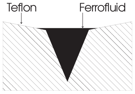
FIG. 2.: Cross-section of the V-shaped teflon channel.

The shadowgraph method [7] is used for detecting the surface waves. The light from a tungsten bulb, placed 50 cm above the center of the channel, is reflected at the surface of the fluid and directed towards the CCD-camera with a glass plate acting as a semitransparent mirror as indicated in Fig. 1. In order to avoid strong nonlinearities of the optical response, the lens of the camera focuses on a plane only a few millimeters above the surface of the fluid. A more precise determination of the focal plane is not necessary because no attempt is made to measure the amplitude of the surface deformation, as this is not considered as an important parameter for these experiments.

The analysis of the images and the control of the experiment is done with a 66 MHz 80486-PC, equipped with a $512\times 512$ 8 bit frame grabber (Data Translation DT2853), a programmable counter (8253) located on a multifunction I/O-board (Meilhaus ME-30), and a synthesizer-board (STAC ASP-ADW1).

The CCD-camera (Phillips LDH 0600/00) works in the interlaced mode at 50 Hz using an exposure time of 40 ms. The time between two horizontal synchronization pulses is $T_{HS}=64$ $\mu$s. The corresponding frequency of $1/T_{HS}=15625$ Hz is divided by the programmable counter. The reduced frequency at the output of the counter acts as a pacer for the synthesizer-board, driving the loudspeaker via an amplifier (Euro Test LAB/S 115).

The camera takes images at a fixed frequency of 25 Hz, while the driving frequency for the surface waves of interest reaches up to 30 Hz. The ensuing problem in resolving the dynamics is overcome by a software-realized stroboscopic image acquisition, which is based on the computer-controlled synchronization between driving and sample frequency.

The stroboscopic image acquisition works in the following way: The period $T_{D}$ of the driving oscillation can only be an integer multiple of the time $T_{HS}$ between horizontal synchronization pulses according to

$\displaystyle T_{D}=N_{SB}M_{C}T_{HS},$

where $M_{C}$ is the multiplier value loaded in the counter, and $N_{SB}$ is the number of data points used by the synthesizer-board to represent the sine wave. The images can only be sampled with a time interval $T_{S}=625$ $T_{HS}=40$ ms, which is the time between two full frames. Consecutive images are taken at times $t_{j}=jT_{S}$, where $j$ represents the number of the image. If one assumes the response of the surface to be periodic with the driving period $T_{D}$, then the surface at time $t_{j}$ is in the same state as at time $t^{\prime}_{j}<T_{D}$, according to:

$$t^{\prime}_{j}(t_{j}) = t_{j}{\rm mod}T_{D}=(jT_{S}){\rm mod}T_{D}$$

$$= ((625j){\rm mod}(N_{SB}M_{C}))T_{HS}.$$

This equation describes the projection of the images taken at the times $t_{j}$ into the time interval $[0,T_{D}[$. The ordering of these images according to increasing $t^{\prime}_{j}(t_{j})$ yields to the reconstruction of one period of the surface motion. The total measurement time $T_{M}$ is the least common multiple of the two periods $T_{D}$ and $T_{S}$. The number of different values of $t^{\prime}_{j}$ is $N_{I}=T_{M}/T_{S}$. The driving frequencies are chosen as a compromise between the desired frequency and sufficient temporary resolution corresponding to $N_{I}\approx 100$.

In order to measure the light intensity along the annulus by means of the frame camera, we divide the circle into 128 segments as schematically indicated in Fig. 3. The mean value of the intensities of those pixels which are located within one segment of the ring is calculated, thus yielding to 128 intensity measurements along the annulus. We consider only odd-numbered lines, which correspond to one half-frame of the camera working in the interlaced mode. The calculations can be performed with the video frequency of 25 frames per second by using a look-up-table technique for the addressing of the pixels of a segment.

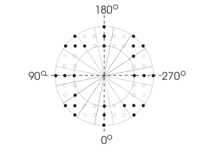
FIG. 3.: The rectangular pixels of the frame camera are assigned to segments along an annulus. Only 16 segments are shown here for clarity; for the measurements we used 128 segments. Note that the number of pixels per segment is not constant.

III Experimental Results

FIG. 4.: Space-time-plot for $B=0$, and $T_{D}=768$ $T_{HS}=49.152$ ms.

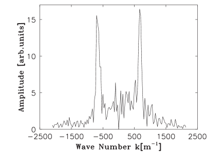
FIG. 5.: Spectrum obtained from Fig. 4. Only wave numbers corresponding to a frequency of $T_{D}^{-1}=20.345$ Hz are shown.

Fig. 4 demonstrates the behavior of a surface wave which is driven at an excitation period $T_{D}=49.152$ ms in the absence of a magnetic field. The horizontal axis represents the 128 intensity values measured along the annulus. The driving occurs at $0^{\circ}$ and $360^{\circ}$, respectively. In this case the stroboscopic algorithm yields 256 measurements per period. These 256 lines are plotted on top of each other according to the sorting algorithm described above. The image displays two waves emanating from the source, travelling clockwise and counterclockwise along the channel. The small amplitude at the position of $180^{\circ}$ results mainly from the attenuation and presumably partly from the interference of the two waves. In order to extract the wave numbers we perform a two-dimensional FFT [8] of this image. In this case this method is artifact-free because we have periodic boundary conditions both in space and in time. The FFT leads to a two dimensional complex field $H(k,\omega)$. The frequency of interest is $\omega_{1}=2\pi/T_{D}$. In Fig. 5 we have plotted $|H(k,\omega_{1})|$ as a function of the 128 available wave numbers. Negative wave numbers represent the wave travelling in clockwise direction, while positive wave numbers correspond to the ones travelling counterclockwise. The spectrum clearly shows two peaks indicating the two dominant waves. The finite size of the peaks is due to the attenuation of the waves. The wave number $k_{P}$ is interpolated between the peak value $|H(k_{max1},\omega_{1})|$ and its largest neighbour $|H(k_{max2},\omega_{1})|$ according to

$\displaystyle k_{P}=\frac{k_{max1}|H(k_{max1},\omega_{1})|+k_{max2}|H(k_{max2},\omega_{1})|}{|H(k_{max1},\omega_{1})|+|H(k_{max2},\omega_{1})|}.$

Measuring $k_{P}$ for different values of the driving period $T_{D}$ then yields to the dispersion relation (see Figs. 9 and 10 below). In principal this experimental procedure would also allow to determine the attenuation of surface waves, provided that our optical setup responds in a linear manner.

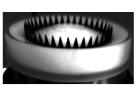
FIG. 6.: Fully developed peaks of a magnetic fluid obtained at $B>B_{c}$ in the annular channel.

If a sufficiently high magnetic field perpendicular to the surface of the magnetic fluid is applied, the normal field instability occurs, leading to characteristic peaks shown in Fig. 6. Because of problems with the aging of the magnetic fluid, the critical magnetic field $B_{c}$ for the onset of this instability drifts in a few weeks from $B_{c}=0.009$ T to $0.011$ T. We thus present all values of the magnetic field in units of the corresponding critical magnetic field.

On the basis of theoretical considerations for the onset of the Rosensweig-Instability [2] one can show that non-monotonic dispersion relations are expected for values of the magnetic field ranging between $0.93$ $B_{c}$ and $B_{c}$. This range is independent of the parameters of the fluid. An example for a non-trivial behavior of the surface waves in this regime is shown in Fig. 7 for a value of the magnetic field of $0.93$ $B_{c}$. This space-time plot displays a clearly more complicated behavior than Fig. 4. It seems to indicate that more than one wave number is excited by the driving period $T_{D}=196.608$ ms. The corresponding spectrum is shown in Fig. 8. The extraction of the dominant wave number is easily obtained, while peaks corresponding to higher wave numbers are much less pronounced and cannot be obtained from this spectrum with reasonable accuracy. We have thus decided to extract only one wave number from the spectra. The results for counter-clockwise travelling waves are summarized in Fig. 9, and for the clockwise waves in Fig. 10. The ordinate of the plot corresponds to the driving frequency, while the abscissa indicates the wave number obtained from the spectra. The results for zero magnetic fields are shown as crosses.

FIG. 7.: Space-time-plot for $B=0.93$ $B_{c}$, and $T_{D}=3072$ $T_{HS}=196.608$ ms.

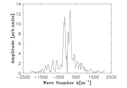
FIG. 8.: Spectrum obtained from Fig. 7. Only wave numbers corresponding to a frequency of $T_{D}^{-1}=5.09$ Hz are shown.

The solid lines in Figs. 9 and 10 are fits of the function $\omega^{2}=ak-bk^{2}+ck^{3}$, where $a$, $b$ and $c$ are fit parameters. The choice of this mathematical form for the fitting function is inspired by the dispersion relation obtained for an inviscid fluid and an infinite layer [2]. There the parameter $a$ would have the value of $g=9.81$ m/s². The mean value of our fit parameter $a$ is $9.96$ m/s². The same theory predicts $b$ to be given by the term $\mu_{0}\mu\frac{(\mu-1)^{2}}{\mu+1}\frac{1}{\rho}H^{2}$. The mean value of $b/H^{2}$ is $2.9\cdot 10^{-10}$ $\frac{\rm m^{4}}{\rm s^{2}A^{2}}$. When using the permeability $\mu=1.8$ provided by the manufacturer of the ferrofluid, one expects $5.1\cdot 10^{-10}$ $\frac{\rm m^{4}}{\rm s^{2}A^{2}}$. The parameter $c$ is theoretically predicted to be $\sigma/\rho=2.6\cdot 10^{-5}$ m³/s² when using the values of the surface tension and the density given above. The measured mean value of $c$ is $2.0\cdot 10^{-5}$ m³/s². In spite of this fairly reasonable agreement it must be stressed that our finite channel is not designed to measure material parameters. There is a visible disagreement between the data and the fitted curves, which are based on an idealized theory. The solid lines are thus basically intended to guide the eye.

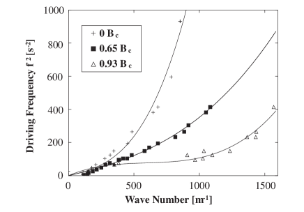
FIG. 9.: Dispersion relation for the waves travelling counter-clockwise.

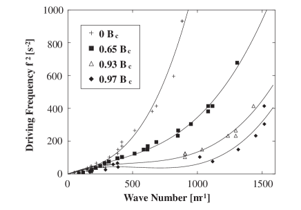
FIG. 10.: Dispersion relation for the waves travelling clockwise.

In increasing the magnetic field the slope of the dispersion relation is reduced. Because of the experimental difficulties described above, we have not attempted to obtain different wave numbers for one given driving frequency, but have rather plotted only the wave number $k_{P}$ of the largest peak. The prediction of a non-monotonic dispersion relation is thus not directly verified by the data points presented in the plot. The fit for $B=0.97$ $B_{c}$ in Fig. 10 shows a local minimum and makes the interpretation of the data points in terms of a non-monotonic dispersion relation very likely. Due to the inhomogeneous magnetic field the corresponding measurement of the waves travelling counter-clockwise was not possible for this value of the magnetic field.

FIG. 11.: Space-time-plot for $B=0.96$ $B_{c}$, and $T_{D}=2240$ $T_{HS}=143.36$ ms.

In order to demonstrate that more than one wave number is indeed present in the parameter range of interest, we finally present in Fig. 11 a measurement for $B=0.96$ $B_{c}$ and a driving period of $T_{D}=143.36$ ms. It clearly shows more than one wave number. In this case the relatively strong attenuation is caused by the longer driving period (compared to Fig. 4). The asymmetry between the left and the right hand side is believed to be caused by the inhomogeneity of the magnetic field, which becomes more dominant close to the critical value $B_{c}$. The corresponding spectrum is shown in Fig. 12. The spectrum might indicate that we reach the limits of our measurement procedure here. It is fairly complex, presumably partly due to the effects of a nonlinear optical response, and effects of field inhomogeneities. In any case at least two peaks are clearly visible for the wave which travels clockwise.

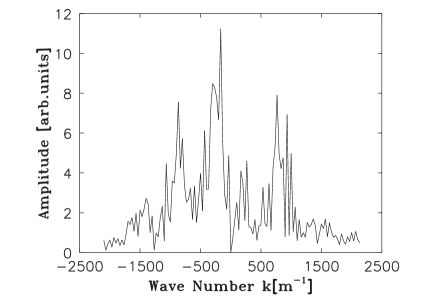
FIG. 12.: Spectrum obtained from Fig. 11. Only wave numbers corresponding to a frequency of $T_{D}^{-1}=6.98$ Hz are shown.

IV Summary and Conclusion

By using a computer-controlled stroboscope algorithm we have measured non-monotonic dispersion relations for a magnetic fluid below the onset of a static pattern forming instability. Due to the finite geometry of our annular channel a quantitative comparison of the experimental results with a theoretical calculation is not possible. Our experiments clearly demonstrate a qualitative similarity with the theory obtained for a inviscous fluid in an infinite layer. Thus, the intriguing possibility arises to parametrically excite [9, 10] three different wave numbers with one single driving frequency, and to study the nonlinear interaction of the ensuing surface waves.

V Acknowledgment

A. G. acknowledges support of MINERVA. The experiments are supported by Deutsche Forschungsgemeinschaft. It is a pleasure to thank H. R. Brand, W. Pesch, H. Riecke and J. Weilepp for stimulating discussions.

REFERENCES

- [1] Proceedings of the Seventh International Conference on Magnetic Fluids, Eds. R. V. Mehta, S. W. Charles, and R. E. Rosensweig, JMMM 149 (1995).
- [2] R. E. Rosensweig, Ferrohydrodynamics (Cambridge University Press, Cambridge 1993).
- [3] G. I. Taylor and A. D. McEwan, J. Fluid Mech. 22 (1965) 1.
- [4] R. E. Zelazo and J. R. Melcher, J. Fluid Mech. 39 (1969) 1.
- [5] V. G. Bashtovoi and R. E. Rosensweig, JMMM 122 (1993).
- [6] J. -C. Bacri, U. d’Ortona, and D. Salin, Phys. Rev. Lett. 67 (1991) 50.
- [7] S. Rasenat, G. Hartung, B. L. Winkler, and I. Rehberg, Experiments in Fluids 7 (1989) 412.
- [8] W. H. Press, B. P. Flannery, S. A. Teukolsky, and W. T. Vetterling, Numerical Recipes in C (Cambridge University Press, Cambridge 1992).
- [9] See M. Cross, and P. C. Hohenberg, Rev. Mod. Phys. 65 (1993) 851, Sec. IX.D for a review. Two more recent examples are e. g. W. S. Edwards, and S. Fauve, J. Fluid Mech. 278 (1994) 123; B. J. Gluckman, C. B. Arnold, and J. P. Gollub, Phys. Rev. E 51 (1995) 1128.
- [10] J. -C. Bacri, A. Cebers, J. -C. Dabadie, and R. Perzynski, Phys. Rev. E 50 (1994) 2712.