Wave-unlocking transition in resonantly coupled complex Ginzburg-Landau equations

Abstract

We study the effect of spatial frequency-forcing on standing-wave solutions of coupled complex Ginzburg-Landau equations. The model considered describes several situations of nonlinear counterpropagating waves and also of the dynamics of polarized light waves. We show that forcing introduces spatial modulations on standing waves which remain frequency locked with a forcing-independent frequency. For forcing above a threshold the modulated standing waves unlock, bifurcating into a temporally periodic state. Below the threshold the system presents a kind of excitability.

Different physico-chemical systems driven out of equilibrium may undergo Hopf bifurcations leading to rich spatio-temporal behavior. When these bifurcations occur with broken spatial symmetries, they induce the formation of wave patterns described by order parameters of the form :

$$\Psi=Ae^{ik_{c}x+i\omega_{c}t}+Be^{-ik_{c}x+i\omega_{c}t}+c.c.$$ (1)

where the slow dynamics of the wave amplitudes $A$ and $B$ obey complex Ginzburg-Landau equations. This is the case, for example, for Rayleigh-Bénard convection in binary fluids, Taylor-Couette instabilities between corotating cylinders, electro-convection in nematic liquid crystals [2], or for the transverse field of high Fresnel number lasers [3]. Symmetry breaking transitions are usually very sensitive to small perturbations or external fields. For example, it has been shown that a spatial modulation of the static electro-hydrodynamic instability of nematic liquid crystals modifies the selection and stability of the resulting roll patterns. In particular, the constraint imposed by a periodic modulation of the instability point may lead to a commensurate-incommensurate phase transition [4]. In the case of Hopf bifurcations, external fields inducing spatial or temporal modulations strongly affect the selection and stability of the resulting spatio-temporal patterns. For example, standing waves may be stabilized by purely temporal modulations at twice the critical frequency [5, 6], or by purely spatial modulations at twice the critical wavenumber [7], in regimes where they are otherwise unstable, including domains where the bifurcation parameter is below the critical one.

External forcings that break space or time translational invariance, but not the space inversion symmetry of the waves amplitudes, induce linear resonant couplings between the complex Ginzburg-Landau equations (CGLE) which describe the dynamics of the amplitudes of left and right travelling waves. In the case of forcings that break the space translation invariance, the coupling coefficient $\epsilon$ is in general complex, and the corresponding coupled CGLE may be written, in one-dimensional geometries, as :

$$\dot{A}+v_{g}\partial_{x}A = \mu A+(1+i\alpha)\partial_{x}^{2}A$$ (2)

$$- (1+i\beta)\left(|A|^{2}+\gamma|B|^{2}\right)A+\epsilon B\>,$$ (3)

$$\dot{B}-v_{g}\partial_{x}B = \mu B+(1+i\alpha)\partial_{x}^{2}B$$ (4)

$$- (1+i\beta)\left(|B|^{2}+\gamma|A|^{2}\right)B+\epsilon A$$ (5)

Due to the resonant coupling with coefficient $\epsilon$, pure travelling waves are not solutions any more of these equations, and generic arguments of bifurcation theory allows a characterization of the possible uniform amplitude solutions depending on the various dynamical parameters of the system [7]. Here also, standing waves may be stabilized as the result of phase locking between the waves $A$ and $B$. Predictions based on (5) in the $x-$independent case have been successfully tested for azimuthal waves in an annulus laser with imperfect O(2) symmetry [8]. However, the combined effect of the complex coupling coefficient $\epsilon$ and the spatial degrees of freedom has not been explored.

In this Letter, we study equations (2) with the following parameter restrictions: imaginary linear coupling coefficient ($\epsilon=i\gamma_{P}$), negligible group velocity $v_{g}$, and weak and real nonlinear cross-coupling term ($\gamma<1$). We will however maintain the spatial derivative in the r.h.s. of (5), and this will be crucial for the results below. We will show that the spatial forcing introduces spatial modulations of the standing waves solutions while $A$ and $B$ remain frequency locked with a forcing-independent frequency. By increasing the forcing, these stable modulated waves merge with unstable ones in saddle-node bifurcations with nontrivial global structure. This wave-unlocking transition results in a mixed state with limit cycle temporal behavior. The threshold value of the forcing and the limit cycle frequency are calculated analytically. Modulated standing waves can also be induced by strong enough temporal forcing [9].

The parameter regime explored here would be appropriate in physical situations where a spatial forcing modulates the frequency of the Hopf instability and induces a purely imaginary resonant forcing (a purely real $\epsilon$ would appear due to a spatial modulation of the distance to the instability point). Possible systems should have negligible group velocities, as in some circumstances in binary fluid convection [10] or liquid crystals [11]; and weak coupling such as in viscoelastic convection [12]. Up to now, the parameter range considered here best applies to several situations in laser physics. A first one corresponds to taking into account transverse effects in inhomogeneously broadened ($\gamma<1$) bidirectional ring lasers [13]. The purely imaginary resonant coupling is a consequence of conservative (off-phase) backscattering [14], or alternatively, a spatial modulation of the refraction index of the laser medium. In fact, a spatially periodic refractive index is the mechanism used for single frequency selection in index coupled Distributed Feedback lasers (DFB). A second situation is that of the transverse vector field in a laser near threshold [15]. The parameter $\gamma_{P}$ corresponds to a detuning splitting between light linearly polarized in different orthogonal directions, produced for example by small cavity anisotropies. In this case, $A$ and $B$ are not the amplitudes of left or right travelling waves, but the amplitudes of the two independent circulary polarized components of light, that is $A=(A_{x}+iA_{y})/\sqrt{2}$ and $B=(A_{x}-iA_{y})/\sqrt{2}$, where $A_{x}$ and $A_{y}$ are the linearly polarized complex amplitudes of the vector electric field with a spatially transverse dependence. Weak coupling ($\gamma<1$) favors linear polarization ($|A|=|B|$). We will often use the light-polarization terminology, because it gives a clear physical insight into the states found for the general set of Eqs. (5) of broad applicability within the parameter restrictions above.

Two families of solutions of the coupled CGLE (5) can be distinguished. The first family corresponds to travelling waves for $A$ and $B$ with the same amplitude, frequency, and wavenumber:

$$A = Q_{0}e^{-ikx+i\omega t+i(\theta_{0}+\psi_{0})}\>,$$ (6)

$$B = Q_{0}e^{-ikx+i\omega t+i(\theta_{0}-\psi_{0})}\>.$$ (7)

Without forcing ($\gamma_{P}=0$), the constant global and relative phases, $\theta_{0}$ and $\psi_{0}$, are arbitrary, the amplitude is $Q_{0}^{2}=(\mu-k^{2})/(1+\gamma)$, and the frequency $\omega$ is $\omega_{0}=-\alpha k^{2}-\beta(1+\gamma)Q_{0}^{2}$. With forcing, the global phase and the amplitude remain unchanged, but the relative phase is fixed by $\sin 2\psi_{0}=0$; the two allowed values of $\psi_{0}$ give two solutions with frequencies $\omega=\omega_{0}\pm\gamma_{P}$. The phase instabilities of these solutions were discussed in [15].

The second family of solutions can be searched in the form of two waves

$$A=e^{i\omega_{0}t}\sum_{n}a_{n}e^{inkx}\ \>,\>\ \ \ B=e^{i\omega_{0}t}\sum_{n}b_{n}e^{inkx}\>,$$ (8)

frequency-locked to a frequency $\omega_{0}$ independent of forcing. For $\gamma_{P}=0$, the exact solutions of (5) in this form only have two terms: $|a_{1}|=|b_{-1}|=Q_{0}$. The effect of a small forcing in this solution is to generate higher harmonics, while keeping $\omega_{0}$ fixed and the relative phase between $a_{1}$ and $b_{-1}$ arbitrary. Now, the remaining coefficients $a_{n}$ and $b_{n}$ are not zero and can be calculated perturbatively in $\gamma_{P}$. Close enough to the threshold for a mode $k$ ($\mu-k^{2}\approx 0$), the amplitude of higher order harmonics is negligible and, to lowest order in $\mu-k^{2}$, an approximate solution takes the form

$$A = e^{i(\theta_{0}+\omega_{0}t)}(Qe^{i(kx+i\psi_{0})}+Re^{-i(kx+\psi_{0}-\phi)})\>,$$ (9)

$$B = e^{i(\theta_{0}+\omega_{0}t)}(Qe^{-i(kx+\psi_{0})}+Re^{i(kx+\psi_{0}+\phi)})\>,$$ (10)

with $\theta_{0}$ and $\psi_{0}$ arbitrary, and $\phi$ fixed by the forcing. $Q$ and $R$ are real numbers (positive or negative) and, for small $\gamma_{P}$, $|R|\ll|Q|$ (an equivalent solution is found interchanging $Q$ and $R$).

A visualization of these solutions can be given within the polarization interpretation of (5). Defining $C_{\pm}e^{i\zeta_{\pm}}\equiv Q\pm e^{i\phi}R$, the change of variables to the amplitudes of the $x-$ and $y-$linearly polarized components gives

$$A_{x}=\sqrt{2}C_{+}\cos(kx+\psi_{0})e^{i(\omega_{0}t+\theta_{0}+\zeta_{+})}\>,$$ (11)

$$A_{y}=\sqrt{2}C_{-}\sin(kx+\psi_{0})e^{i(\omega_{0}t+\theta_{0}+\zeta_{-})}\>,$$ (12)

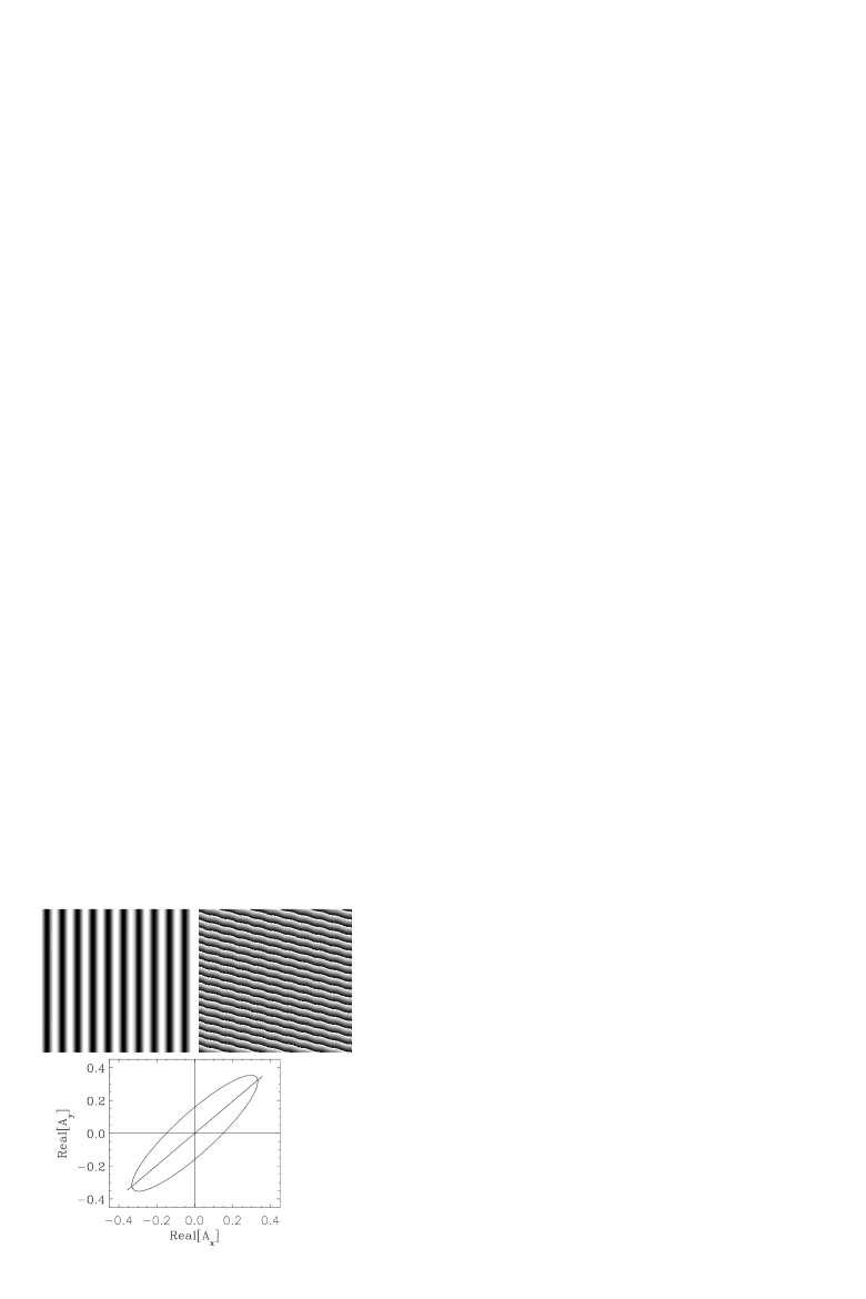
FIG. 1.: Top: Modulus (left) and phase (right) of $A$ for $\gamma_{P}=0.012<\gamma_{Pc}$. The horizontal axis is space (256 units), and the vertical is time (1000 units). Gray levels range from black (0) to white (the maximum of the modulus or $2\pi$ for the phase). This numerical solution has been obtained from (2) with $\beta=0.2$, $\gamma=0.5$, $\mu=0.2$, $\alpha=2.6$. The initial condition is a standing wave with $\omega=\omega_{0}$ and $k=0.123$. Bottom: Polarization representation of the solution at a given point $x$. For $\gamma_{P}=0$ one has linear polarization (indicated by the straight line) which becomes elliptical for $\gamma_{P}\not=0$. An equivalent solution has the major axis of the ellipse along the second and fourth quadrants.

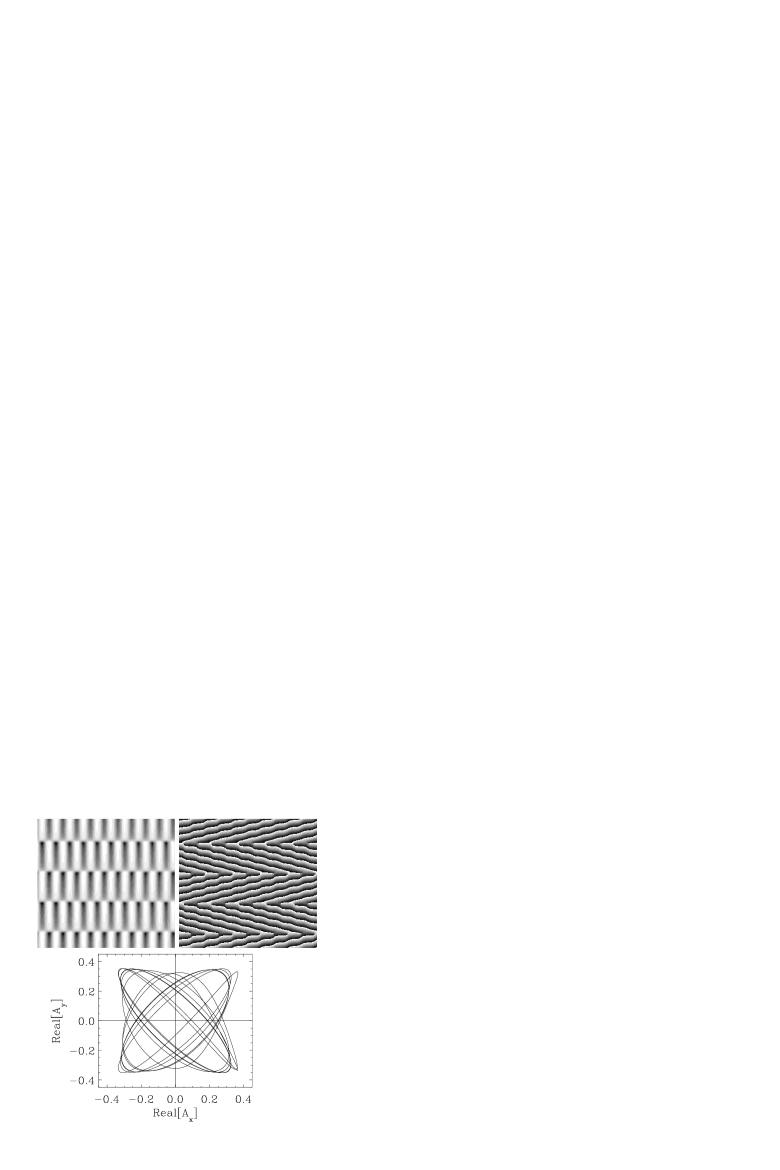
FIG. 2.: Same as Fig. 1 but using $\gamma_{P}=0.0145>\gamma_{Pc}$.

These equations describe at each point $x$ the superposition of two dephased harmonic motions with different amplitudes and a frequency $\omega_{0}$ independent of forcing. This identifies the solution (10) with an elliptically polarized standing wave pattern in which the orientation of the ellipse and its ellipticity vary periodically in the spatial coordinate $x$. In the limit of no forcing, $R=0$, the ellipse degenerates in a linearly polarized standing wave with an angle of polarization $\psi=kx+\psi_{0}$. In this interpretation, the first family of solutions, (7), would correspond to linearly polarized traveling waves with frequency $\omega$ and an angle of polarization $\psi_{0}$. In such a case, the forcing fixes the direction of polarization so that only $x$- or $y$-linearly polarized waves remain. On the contrary, forcing in (10) grows an ellipse from a linearly polarized standing wave keeping the frequency unchanged.

Elliptically polarized standing wave patterns are obtained from a direct numerical integration of the coupled CGLE as shown in Fig. 1. Increasing the forcing, these solutions become unstable through a bifurcation in which $Q$ and $R$ become time dependent. As shown in Fig. 2, the solution beyond this instability oscillates between the two equivalent elliptically polarized standing wave patterns found for small $\gamma_{P}$. In addition, from the numerical simulations, one finds that the period $T$ of these oscillations decreases beyond the critical value $\gamma_{Pc}$. One has $T^{-2}\propto(\gamma_{P}-\gamma_{Pc})$ (see Figs. 3 and 4).

A quantitative description of the instability, including the determination of the critical forcing $\gamma_{Pc}$ and the period of the oscillations, can be performed by an amplitude analysis. Close to the threshold for the $k$ modes, the equations for the slow time evolution of $Q$ and $R$ can be found by substitution of (10) into (5) and neglecting contributions from higher order harmonics. Defining $Xe^{i\Phi}\equiv Q+iR$ we find

$$\dot{X} = (\mu-k^{2})X-(1+\gamma)X^{3}-(1+\gamma\cos 2\phi){X^{3}\over 2}\sin^{2}2\Phi\>,$$ (13)

$$\dot{\Phi} = -(1+\gamma\cos 2\phi){X^{2}\over 2}\sin 2\Phi\cos 2\Phi$$ (14)

$$+ \beta\gamma\sin 2\phi{X^{2}\over 2}\sin 2\Phi-\gamma_{P}\sin\phi\>,$$ (15)

$$\dot{\phi} = \beta(1+\gamma\cos 2\phi)X^{2}\cos 2\Phi+\gamma X^{2}\sin 2\phi$$ (16)

$$- 2\gamma_{P}\cos\phi\cot 2\Phi\>.$$ (17)

The fixed points of (17) represent the polarized standing waves solutions (10). These points can be determined exactly in the limiting case of $\beta=0$. The interesting solutions have two allowed values of $\phi$: $\phi_{0}=(2n+1)\pi/2$, $n=0$, $1$; and for each value of $\phi$, there are eight fixed points: Four are stable ($+$) and the other four are saddle points ($-$). The corresponding values of $X$ and $\Phi$ are:

$$X_{0}(\pm)^{2} = {\mu-k^{2}\over 2(3+\gamma)(1+\gamma)}$$ (18)

$$\!\!\!\!\!\!\!\!\!\!\left[5+3\gamma\pm\sqrt{(1-\gamma)^{2}-{8(1+\gamma)(3+\gamma)\gamma_{P}^{2}\over(\mu-k^{2})^{2}}}\right]\>,$$ (19)

$$\Phi_{0}(+)=\xi(+)+m\frac{\pi}{2},\ \Phi_{0}(-)=\frac{\pi}{4}-\xi(-)+m\frac{\pi}{2}\ ,$$ (20)

where $m=0,1,2,3$, and

$$\xi(\pm)={(-1)^{n+1}\over 4}\arcsin{4\gamma_{P}\over(1-\gamma)X_{0}(\pm)^{2}}\>.$$ (21)

Heteroclinic orbits connect the saddles and the stable nodes with the same $\phi$. When $\gamma_{P}$ grows, saddles and nodes approach by pairs and at the critical value

$$\gamma_{Pc}={(\mu-k^{2})(1-\gamma)\over\sqrt{8(1+\gamma)(3+\gamma)}}\>,$$ (22)

they merge and disappear via inverse saddle node bifurcations. The interesting point is the global structure of the bifurcation: the presence of the heteroclinic connections gives rise to the birth of limit cycles (one for each value of $\phi$). This is similar to the Andronov-van-der-Pol bifurcation [16] that appears in several types of excitable systems [17]. The difference is that, due to symmetries, here we have several pairs of fixed points merging, instead of just one pair. The periodic behaviour is illustrated in Fig. 2 by the periodic alternation of the trajectory between the “ghosts” of the disappeared elliptically polarized states corresponding to the fixed points. Below the bifurcation, small perturbations around the stable solutions decay, whereas perturbations above a threshold push the system along the heteroclinic trajectory towards another stable fixed point. Since the size of the perturbation required for such switches decreases by increasing $\gamma_{P}$, and vanishes at $\gamma_{Pc}$, the multistability of this system can be seen as a kind of excitability [18]. A different consequence of the multiplicity of stable states is their possible coexistence in space, leading to the formation of domains with different polarizations along the $x$ axis.

FIG. 3.: Period of the oscillations ($T$) of $Q$ and $R$ obtained from the numerical solution of the coupled CGLE using the parameters given in Fig. 1. The dashed line is a least squares fitting from which $\gamma_{Pc}=0.0138$.

FIG. 4.: The amplitudes of $Q$ and $R$ of the solution shown in Fig. 2 exhibit the periodic oscillations given by Eq. (13). The time has been scaled using the value of $\gamma_{Pc}$ obtained from Fig. 3. The dotted line corresponds to $\gamma_{p}=0.0155$, the dashed line to $\gamma_{p}=0.0140$, and the lines in between to the other points of Fig. 3.

Close to the instability at $\gamma_{Pc}$, the time dependent behavior of the solution can be obtained reducing the problem to a phase dynamics by elimination of the variable $X$. We have (in the limit $\beta=0$),

$$\dot{\Phi} = -{(\mu-k^{2})(1-\gamma)\sin 4\Phi\over 5+3\gamma-(1-\gamma)\cos 4\Phi}+\gamma_{P}\>,$$ (23)

which for $\gamma_{P}\geq\gamma_{Pc}$ yields the following time behavior:

$$\tan(2\Phi) = \tan(2\Phi_{c})\left(1+\sqrt{2(\gamma_{P}-\gamma_{Pc})/\gamma_{Pc}}\right.$$ (25)

$$\left.\tan\left((5+3\gamma)\sqrt{\gamma_{Pc}}\sqrt{\frac{\gamma_{P}-\gamma_{Pc}}{(1+\gamma)(3+\gamma)}}\>t\right)\right)\>.$$

where, $\Phi_{c}=\Phi_{o}$, Eq. (20), for $\gamma_{P}=\gamma_{Pc}$.

An approximative analysis of Eqs. (17) for $\beta\neq 0$ indicates that this parameter appears squared in the expressions for $\gamma_{Pc}$, $X$ and $\Phi_{c}$. Therefore, for small $\beta$, the previous analysis is still meaningful as explicitly seen in the numerical results of Figs. 3 and 4.

In summary, in the absence of forcing, and for the parameter regime considered here, there are solutions for the amplitudes $A$ and $B$, of the coupled CGLE which correspond to linearly polarized standing waves. We have shown that an imaginary coupling between them transforms these solutions into standing waves with spatially periodic elliptic polarization. Increasing the forcing, an instability of these solutions, via the unlocking of the underlying wave amplitudes, appears and the solutions acquire a time-periodic behavior. Locally, this bifurcation is of the saddle-node type, but the presence of heteroclinic connections between the fixed points gives rise to the appearance of a limit cycle when stable and unstable points merge.

Financial support from DGICYT Projects PB94-1167 and PB94-1172 is acknowledged.

REFERENCES

- [1] Director of Research at the Belgian National Fund for Scientific Research. Center for Nonlinear Phenomena and Complex Systems, Université Libre de Bruxelles, Campus Plaine, Blv. du Triomphe B.P 231, 1050 Bruxelles.
- [2] M.C. Cross and P.C. Hohenberg, Rev. Mod. Phys. 65 , 854 (1993).
- [3] A.C. Newell and J.V. Moloney, Nonlinear Optics (Addison-Wesley, Redwood City, 1992 ).
- [4] M. Lowe and J.P. Gollub, Phys. Rev., A31, 3893 (1985).
- [5] D. Walgraef, Europhys.Lett., 7, 485 (1988).
- [6] H.Riecke, J.D.Crawford and E.Knobloch, Phys. Rev. Lett. , 61, 1942 (1988).
- [7] G. Dangelmayr and E. Knobloch, Nonlinearity 4, 399 (1991).
- [8] E.J. D’Angelo, E. Izaguirre, G.B. Mindlin, G. Huyet, L. Gil, and J.R. Tredicce, Phys. Rev. Lett. 68, 3702 (1992).
- [9] S. Douady, S. Fauve and O. Thual, Europhysics Letters, 10, 309 (1989).
- [10] P. Kolodner, Phys. Rev. A 44, 6448 (1991); Phys. Rev. Lett. 66, 1165 (1991).
- [11] S. Kai ed., Physics of Pattern Formation in Complex Dissipative Systems, World Scientific, Singapour (1992).
- [12] J. Martínez-Mardones, R. Tiemann, W. Zeller, and C. Pérez-García, Int. J. Bifurc. Chaos 4, 5 (1994).
- [13] S. Singh, Phys. Rep. 108, 217 (1984).
- [14] C. Etrich, P. Mandel, R. Neelen, R.J.C. Spreeuw, J.P. Woerdman, Phys. Rev. A 46, 525 (1992).
- [15] M. San Miguel, Phys. Rev. Lett. 75, 425 (1995).
- [16] A.A. Andronov, A.A. Vitt and S.E. Khaikin, Theory of oscillators, Pergamon Press, Oxford (1966).
- [17] S.C. Mueller, P. Coullet and D. Walgraef, chaos 4, 3, 439 (1994).
- [18] E. Meron, Phys. Rep. 218, 1 (1992).