Coarse-grained description of thermo-capillary flow

Abstract

A mesoscopic or coarse-grained approach is presented to study thermo-capillary induced flows. An order parameter representation of a two-phase binary fluid is used in which the interfacial region separating the phases naturally occupies a transition zone of small width. The order parameter satisfies the Cahn-Hilliard equation with advective transport. A modified Navier-Stokes equation that incorporates an explicit coupling to the order parameter field governs fluid flow. It reduces, in the limit of an infinitely thin interface, to the Navier-Stokes equation within the bulk phases and to two interfacial forces: a normal capillary force proportional to the surface tension and the mean curvature of the surface, and a tangential force proportional to the tangential derivative of the surface tension. The method is illustrated in two cases: thermo-capillary migration of drops and phase separation via spinodal decomposition, both in an externally imposed temperature gradient.

I Introduction

The study of multi-phase flows leads to a classical moving boundary problem in which the equations governing fluid motion are solved in each phase, subject to boundary conditions specified on the moving boundaries. In the classical case, the boundary of separation is assumed to be an idealized boundary without any structure. For viscous flows, the velocity field is continuous across the boundary, whereas the normal component of the stress tensor is discontinuous if capillary forces are allowed for. Implicit in this formulation are, of course, assumptions that local thermodynamic equilibrium obtains and that the typical length scales of spatial structures and flow are much larger than the scale of the physical boundary separating the phases. In most cases of interest to fluid mechanics the scale of the flow is set externally by macroscopic stresses on the system, whereas the length scale of the interface is of microscopic size and set by the range of the intermolecular forces in the fluid. Under these conditions, the transition region between the two phases can be approximated for all practical purposes by an ideal, mathematical surface of discontinuity.

A notable exception to this rule concerns flow in a fluid near or at its critical point. There the surface of separation between both phases becomes arbitrarily diffuse, and the flow within the boundary itself needs to be explicitly modeled and resolved. The so-called Model H (following the nomenclature of Hohenberg and Halperin [1]) was introduced to study order parameter and momentum density fluctuations near the critical point, as well as their interaction, at a coarse-grained or mesoscopic scale [2]. Additional (reversible or Hamiltonian) terms were added on phenomenological grounds to the Navier-Stokes equation and to the equation governing the relaxation of fluctuations in the order parameter appropriate for the phase transition under consideration. Later studies based on the same model have addressed critical fluctuations of simple fluids [3, 4] and polymers [5, 6] under external shear, and more recently (and more closely related to our study) hydrodynamic effects on spinodal decomposition in a binary fluid [7, 8]. In spinodal decomposition, a binary system is quenched from a homogeneous disordered state to a region of the phase diagram in which the homogeneous state is linearly unstable to fluctuations in a wide band of length scales. (For a review, see, e.g., [9].) Some further details on the general principles behind a mesoscopic description of equilibrium properties of bulk phases and of interfacial structures can be found in readily available texts and monographs (see, e.g., Refs [10, 11, 12, 13, 14].) Implications of such a level of description on the equations governing fluid flow are discussed in the appendix, where the modifications of the non-dissipative part of the stress tensor embodied in Model H are obtained. This “Hamiltonian” or reactive part of the stress tensor does not contribute to the entropy increase. Additional treatments based on irreversible thermodynamics and continuum mechanics can be found in Refs. [15, 16].

The usefulness of a coarse-grained approach away from a critical point is less well established. Previous work along these lines includes Ginzburg-Landau models used in the study of the kinetics of phase separation (e.g., the Cahn-Hilliard equation) [9], or phase field models of solidification [17, 18, 19]. In both cases, a mathematical surface of separation between the two phases becomes a transition region of small but finite width, across which all magnitudes change continuously. The essential ingredient in both cases is the assumption that the relevant thermodynamic potential density (entropy in closed systems, Helmholtz free energy if the system is held at constant temperature) is a function not only of the usual thermodynamic variables and of the order parameter, but also of the spatial gradient of the latter. In the case of a binary fluid, for example, the entropy density is assumed to depend on both the mass density of solute and its spatial derivative. As a consequence, the chemical potential of the solute is no longer given by the derivative of the local entropy with respect to solute density.

From a theoretical point of view, it is plausible to assume that modes describing the motion of boundaries separating bulk phases, even away from a critical point, are the long-lived modes of the dynamics of the system, and hence gradients of the order parameter can be considered as additional arguments upon which the thermodynamic potential depends, at least on the time scale over which the motion of the boundaries is observable macroscopically. Furthermore, one would also like to satisfy the consistency requirement that the coarse-grained model reduces to the classical macroscopic description in the limit of a small transition region (compared to the scale of relevant structures). This requires, in general, relating macroscopically measurable quantities (e.g., the surface tension of the boundary) to phenomenological parameters that enter the mesoscopic model [20].

One of the chief advantages of a mesoscopic approach is that it allows the study of fluid phenomena that lie outside the classical continuum formulation, for example, the break up and coalescence of fluid domains. More generally, by incorporating explicitly into the model dissipation at short length scales (on the order of the interfacial thickness or order parameter correlation length), the model allows the study of other physical situations that may be influenced by phenomena at that scale. Other examples that may fall in this class include motion of contact lines, flow near solid walls and slip at a microscopic or mesoscopic scale.

From a purely computational point of view the model used can be viewed as an extension of a class of numerical methods often used to study the classical moving boundary problem, namely, those that phenomenologically introduce additional dissipation at short length scales. At least in principle, however, the method that we describe in this paper differs from those approaches (e.g., methods based on the introduction of ad-hoc “artificial dissipation” or “artificial viscosity”), since, in the present case, short length scale dissipation is intrinsically part of the model, and is related to the order parameter variable that describes the phases. Also from a computational point of view, the approach that we follow is similar to the so-called immersed boundary or diffuse interface methods introduced for the study of multi-phase flows [21, 22, 23, 24, 25]. The order parameter which we define below plays a role analogous to the “color function.” However, it is not an auxiliary field introduced for computational convenience, but rather a thermodynamic variable in its own right, controlled by a local free energy density. As a consequence, for example, the surface tension of this model cannot be fixed independently, but is completely determined by the choice of thermodynamic potential and the parameters contained therein. This will reveal some interesting features to be expected at high thermal gradients.

In Section II we introduce the coarse-grained model used in our study. We concentrate in this work on thermo-capillary flows and hence explicitly discuss how to couple the equation governing fluid motion and relaxation of the order parameter. In this paper we will consider the case of a constant, externally imposed temperature gradient, although it is straightforward to extend our calculations to incorporate a fluctuating temperature field. We also discuss in this section the limit of a thin interface and the boundary conditions that result from our model in that limit. As illustrations, we apply the numerical approach to two problems of interest. In Section III thermo-capillary motion of small drops under large thermal gradients is considered, while in Section IV we study phase separation via spinodal decomposition in the presence of a uniform temperature gradient. Section V is reserved for concluding remarks. An appendix provides additional details on the derivation of modifications to the Navier-Stokes equation introduced through the coarse-grained level of description.

II Coarse-grained model

A Formulation

Consider an incompressible and Newtonian binary fluid at a temperature below its phase separation critical point. Let $\varphi$ be the order parameter density appropriate for the un-mixing transition, chosen to be $\varphi=0$ in the disordered phase above the transition point, and symmetric and equal to $\pm\varphi_{eq}$ below. [$\varphi$ can be thought of as $c-c_{c}$, where $c$ is the mass fraction of one of the species and $c_{c}$ its value at the phase separation critical point.] One further makes the reasonable assumptions for binary liquid systems that the shear viscosities of both phases are equal, and that the dependence of the mass density on the order parameter is weak and can be neglected. In effect, we consider here a “symmetric” model in which all bulk properties of both phases are equal. These restrictions, which conveniently dramatize interfacial phenomena in the cases which we study here, can be easily removed.

If $\vec{v}$ is the velocity of an element of fluid, conservation of mass and momentum lead to,

$$\nabla\cdot\vec{v}=0,$$ (1)

$$\rho\frac{d\vec{v}}{dt}=-\nabla p+\eta\nabla^{2}\vec{v}+\mu\nabla\varphi,$$ (2)

where $\mu=\delta{\cal F}/\delta\varphi$ is the chemical potential conjugate to the order parameter $\varphi$ ($\delta/\delta\varphi$ stands for functional or variational differentiation), $\rho$ and $\eta$ are the density and shear viscosity of the fluid respectively, and $p$ is the pressure field. The last term in Eq. (2) is non-standard in macroscopic approaches and incorporates capillary effects as discussed further below and in the appendix. As a reference, we note that the Navier-Stokes equation is also modified in Immersed Boundary Methods by adding a term of the form,

$$\left(\sigma\kappa\hat{n}+\frac{\partial\sigma}{\partial s}\hat{s}\right)\delta\left(\vec{x}-\vec{x}_{S}\right),$$ (3)

where $\vec{x}_{S}$ is the instantaneous location of the boundary. Here $\sigma$ is the interfacial tension (independently prescribed), $\hat{n}$ and $\hat{s}$ are the unit vectors along the normal and tangential directions respectively, and $\kappa$ is the mean curvature of the interface. As we further discuss in Section II B, the term $\mu\nabla\varphi$ in Eq. (2) in the limit of a thin interface reduces to the term used in Immersed Boundary Methods, but with $\sigma$ now determined by the coarse-grained free energy functional ${\cal F}$ (see, e.g., Refs [10, 11, 12, 13, 14]) that, for simplicity, is chosen to be of the form,

$${\cal F}\left[\varphi\right]=\int dV\left\{\frac{K}{2}|\nabla\varphi|^{2}+f(\varphi)\right\},$$ (4)

with,

$$f(\varphi)=-\frac{r}{2}\varphi^{2}+\frac{\lambda}{4}\varphi^{4}.$$ (5)

The integration extends over the entire system (both bulk phases and interfacial regions), and $K,r,$ and $\lambda$ are three phenomenological coefficients as yet unspecified, other than requiring $K,\lambda>0$. For the model defined by Eqs. (4) and (5) the chemical potential is given by $\mu=-K\nabla^{2}\varphi-r\varphi+\lambda\varphi^{3}$. As is well known, this free energy qualitatively describes a single homogeneous phase over a range of parameters ($r<0$) yielding to two-phase coexistence in another region ($r>0$). The parameter $r$ is therefore a measure of distance below the phase separation critical temperature and is taken to be proportional to that temperature difference, while the parameter $\lambda$, at this level of approximation can be related to the inter-particle potentials (or to a virial coefficient). As noted below, the parameters $\lambda$ and $K$ can be determined from equilibrium measurements. The order parameter is further assumed to satisfy a modified Cahn-Hilliard equation,

$$\frac{\partial\varphi}{\partial t}+\nabla\cdot\left(\varphi\vec{v}\right)=M\nabla^{2}\mu$$ (6)

to allow for advective transport of $\varphi$. $M$ is a phenomenological mobility coefficient of microscopic origin, which, in a real system, could be inferred from mutual diffusion and order-parameter susceptibility measurements away from the critical region.

Equations (1)-(2) and (4)-(6) completely specify the model. We have imposed the following boundary conditions at the edges of the fluid domain: $\vec{v}=0$, $\varphi=\varphi_{eq}(T)$, and $\partial\varphi/\partial n=\partial\varphi_{eq}(T)/\partial n$, i.e., the value of the order parameter near the boundary is determined by the imposed temperature field there. Note that with this choice of boundary conditions, $\int dV\varphi$ is not a strictly conserved quantity. The boundary conditions required to enforce strict conservation of order parameter are $\partial\varphi/\partial n=0$ and $\partial\nabla^{2}\varphi/\partial n=0$. In this case small boundary layers of $\varphi$ (of thickness of the order of the correlation length $\xi$) would develop because $\varphi$ in the bulk (and away from interfaces) is approximately equal to $\varphi_{eq}(T)$, and therefore would not satisfy this latter set of boundary conditions. Our choice of boundary conditions is motivated by computational simplicity so that we do not have to resolve additional boundary layers at the edges of the domains. In any event, the spatial integral of $\varphi$ changes very little during the course of the numerical solution, and hence this choice has little effect on the dynamics in the bulk phases.

From Eq. (5) one finds $\varphi_{eq}=\sqrt{r/\lambda}$ with $\pm\varphi_{eq}$ as the two coexisting solutions. Equation (6) also admits a nonuniform, “kink” stationary solution for $\vec{v}=0$ and constant $r>0$,

$$\varphi_{0}(u)=\varphi_{eq}\tanh\frac{u}{\sqrt{2}\xi},$$ (7)

with boundary conditions $\varphi\rightarrow\pm\varphi_{eq}$ as $u\rightarrow\pm\infty$. The coordinate $u$ is along an arbitrary direction and $\xi$ is the mean field correlation length, $\xi=\sqrt{K/r}$. This stationary solution represents the coexistence of two equilibrium phases with $\varphi=\pm\varphi_{eq}$, across a transition region located at $u=0$ and of width $\xi$. In what follows, we will refer to the regions $|u/\xi|\gg 1$ as the bulk phases, and $|u/\xi|\sim 1$ as the interfacial or transition region. In the region of parameters of Eqs. (4) and (5) that we explore, the surface area occupied by the bulk phases is much larger than that of the interfaces.

The excess free energy density associated with Eq. (7) compared to the free energy of either uniform phase is given by [14],

$$\sigma=K\int_{-\infty}^{\infty}du\left(\frac{d\varphi_{0}}{du}\right)^{2}=\frac{2K\varphi_{eq}^{2}}{3\xi}.$$ (8)

We introduce dimensionless variables by choosing $\xi$ as the scale of length, $K/Mr^{2}$ as the scale of time, and $\varphi_{eq}$ as the order parameter scale. In dimensionless units, the model equations reduce to,

$$\nabla\cdot\vec{v}=0,$$ (9)

$${\rm Re}\frac{d\vec{v}}{dt}=-\nabla p+\nabla^{2}\vec{v}+{\rm C}\left(-\nabla^{2}\varphi-\varphi+\varphi^{3}\right)\nabla\varphi,$$ (10)

and,

$$\frac{\partial\varphi}{\partial t}+\nabla\cdot(\varphi\vec{v})=\nabla^{2}\left(-\nabla^{2}\varphi-\varphi+\varphi^{3}\right).$$ (11)

Two dimensionless groups remain; one of them, Re$=Mr/\nu$ ($\nu=\eta/\rho$ is the kinematic viscosity) gives the ratio between order parameter diffusion and momentum diffusion due to viscosity. In the calculations that we describe in this paper, the system is in the overdamped limit of Re$\simeq 0$. The other, C$=3\sigma\xi/2\eta Mr$, plays the role of a capillary number. Flows in our study are entirely driven by surface tension. In the overdamped limit the velocity scale of such flows is $v\sim\sigma/\eta$ where we have assumed that the scale of the flow is the same as the scale of the typical domains of the two phases. Therefore, the characteristic time for an element of fluid to be advected a distance equal to the interfacial thickness is $\tau_{\sigma}=\xi\eta/\sigma$. The diffusive time scale given above is $\tau_{\varphi}=\xi^{2}/Mr$; hence C $\propto\tau_{\varphi}/\tau_{\sigma}$.

In order to couple the previous equations to a slowly varying temperature field, we make, as noted above, the traditional identification of the parameter $r$ in Eq. (4) as being a linear function of temperature $r(\vec{x})\propto T_{0}-T(\vec{x})$, where $T_{0}$ is a constant playing the role of the consolute or critical temperature. In the case that we study, the temperature field is fixed and remains constant throughout the calculation. If one wishes to incorporate a fluctuating temperature field, the model equations have to be supplemented with the equation of energy conservation [26]. In dimensionless units, we consider,

$$\frac{\delta{\cal F}}{\delta\varphi}=-\nabla^{2}\varphi-\tau(y)\varphi+\varphi^{3},$$ (12)

where the dimensionless local temperature variable $\tau(y)=\tau_{0}+\alpha y$, with $\alpha$ the dimensionless temperature gradient. We identify the $y-$direction as the direction in which the imposed temperature varies. For our coarse grained analysis to make sense we require that temperature variations are small over small distances (of the order of the interfacial thickness), namely, in dimensionless form, $|\alpha|\ll 1$, but perhaps large over distances of the order of the system size, and possibly even over a domain of one of the phases.

B Sharp interface limit

We next present a heuristic analysis to illustrate that the coarse-grained model introduced reduces to the classical continuum description in the limit in which the width of the interfacial region is much smaller that the size of the bulk domains. We introduce a local orthogonal system $(s,u)$ such that a given point in space is given by $\vec{r}=\vec{R}(s)+u\hat{n}$, where $\vec{R}(s)$ describes the location of the level set $\varphi(\vec{r})=0$ ($s$ is the arclength along it), $\hat{n}$ is the local normal pointing towards the (+) phase, and $u$ is the distance along the normal direction.

In the bulk regions ($|u/\xi|\gg 1$) $\mu\nabla\varphi$ is of order higher than linear in the gradients and therefore negligible. One then recovers the standard Navier-Stokes equation. The Cahn-Hilliard equation can be likewise linearized around $\varphi_{eq}$ in the bulk regions, yielding the standard diffusion equation with advective transport.

In the interfacial regions ($|u/\xi|\sim 1$), the term $\mu\nabla\varphi$ does become large. In the limit of gently curved interfaces, $|\kappa\xi|\ll 1$, where $\kappa$ is the mean curvature of the interfacial region, and for small temperature gradients, $|\alpha|\ll 1$, the field $\varphi$ relaxes on a fast time scale to essentially the stationary solution $\varphi_{0}(u)$ as in Eq. (7)  [29]. One can develop a multiscale expansion of the field $\varphi=\varphi(S,u,U)$ with $S,U$ the slowly varying coordinates in the tangential and normal direction as set by the slow variation of the temperature field, and $u$ the fast variation in the normal direction as determined by the free energy functional. We further assume – and this remains to be proven more rigorously – that $\varphi$ relaxes quickly to its local equilibrium profile given by the local value of the temperature, but there remain slow gradients of $\varphi$, since this approximate solution is no longer a solution of $\delta{\cal F}/\delta\varphi=~{}\mbox{constant},$ throughout the system. The surface tension in Eq. (8) can then be written as,

$$\sigma=\int_{-\infty}^{+\infty}du\Delta F(u,U,S),$$ (13)

where $F=\frac{1}{2}K|\nabla\varphi|^{2}+f(\varphi)$ and $\Delta F$ is the free energy (density) difference between the mean field value of $F$ at the local value of $\varphi$ in a configuration with a two-phase interface and the free energy of the bulk phases $\varphi_{eq}$, at the local temperature. Under the assumptions stated above, this expression can be used to define a slowly varying surface tension $\sigma(S)$ along the interface, since the magnitude of the order parameter $\varphi$ will be the local equilibrium value at the local temperature. Then,

$$\frac{\partial\sigma}{\partial S}=\int_{-\infty}^{\infty}du\left(\frac{\partial F_{int}}{\partial\varphi}\right)\frac{\partial\varphi}{\partial S}=\int_{-\infty}^{\infty}du\mu\frac{\partial\varphi}{\partial S}\,\,,$$ (14)

where we have used the fact that the metric tensor element $g_{22}=\frac{d\vec{r}}{ds}\cdot\frac{d\vec{r}}{ds}=(1+u\kappa)^{2}\approx 1$ in the limit of gently curved interfaces considered. (Note that $\kappa<0$ for a sphere). The chemical potential appearing is appropriate for an interfacial configuration and is non-vanishing for a gently curved (or indeed a flat) interface in a temperature gradient. Hence the tangential component of $\mu\nabla\varphi$ gives rise to a tangential surface force which equals the tangential derivative of the surface tension.

We can likewise study the normal component by recalling that,

$$\int_{-\infty}^{\infty}du\mu\frac{\partial\varphi}{\partial u} = \int_{-\infty}^{\infty}du\left[-\nabla^{2}\varphi+f^{\prime}\right]\frac{\partial\varphi}{\partial u}$$ (15)

$$\simeq \int_{-\infty}^{\infty}du\left[-\frac{\partial^{2}\varphi}{\partial u^{2}}-\kappa(S)\frac{\partial\varphi}{\partial u}-\frac{\partial^{2}\varphi}{\partial S^{2}}+f^{\prime}\right]\frac{\partial\varphi}{\partial u}$$ (16)

$$\simeq \kappa(S)\int_{-\infty}^{\infty}du\left(\frac{\partial\varphi}{\partial u}\right)^{2}-\int_{-\infty}^{\infty}du\frac{\partial^{2}\varphi}{\partial S^{2}}\frac{\partial\varphi}{\partial u}.$$ (17)

The first term gives again the surface tension $\sigma$, and the second term would remain in the sharp interface limit due to the slow variation of $\varphi$ with temperature.

Therefore in the case of a thin interfacial region, the additional term in the Navier-Stokes equation is equivalent – under the stated assumptions of a slowly varying temperature field and gently curved interfaces – to a tangential surface force proportional to the tangential derivative of the surface tension, and to a normal force proportional to the mean curvature of the interface.

C Numerical method

We next discuss the numerical algorithm used in the actual computations. We restrict our attention in this paper to two dimensional flows. Since the velocity field is solenoidal, it is convenient to introduce the stream function,

$$\vec{v}=\nabla\times(\psi\hat{k})=\frac{\partial\psi}{\partial y}\hat{i}-\frac{\partial\psi}{\partial x}\hat{j},$$ (18)

where the velocity field is defined in the $(x,y)$ plane, and $\hat{k}$ is the unit normal perpendicular to that plane. By taking the curl of Eq. (10) with Re = 0 we find,

$$\nabla^{4}\psi+{\rm C}\left[\nabla\left(\nabla^{2}\varphi\right)\times\nabla\varphi\right]\cdot\hat{k}=0.$$ (19)

The flow field can be found by solving a biharmonic equation for the stream function, subject to the boundary conditions that both the stream function $\psi$ and its normal derivative $\partial\psi/\partial n$ vanish on the external boundaries of the system.

Concerning the equation for the order parameter, Eq. (11), we follow Ref. [30] and use a backward implicit method which is first order in time,

$$\frac{\varphi(t+\Delta t)-\varphi(t)}{\Delta t}+\nabla\cdot(\vec{v}(t)\varphi(t+\Delta t))=-{\cal L}\varphi(t+\Delta t)+\nabla^{2}\varphi^{3}(t+\Delta t),$$ (20)

with ${\cal L}=\nabla^{4}+\nabla^{2}$. The convective term has been kept in conservative form, and the velocity field retained in the discretization is at time $t$. The boundary conditions that we use for the order parameter are $\varphi=\varphi_{eq}(T)$ and $\partial\varphi/\partial n=\partial\varphi_{eq}(T)/\partial n$ on the external boundaries. A Gauss-Seidel iteration is used to solve Eq. (20). First, one considers an “outer” iteration,

$$\varphi(t+\Delta t)\simeq\varphi_{k+1}=\varphi_{k}+\delta_{k}\quad{\rm with}\quad\varphi_{0}=\varphi(t).$$ (21)

Substituting $\varphi(t+\Delta t)$ in Eq. (20) and linearizing in the outer correction field $\delta_{k}(x,y)$ yields an equation for the outer correction with a residual that is a function of $\varphi_{k}$. Successive iterates converge to a solution when both the residual and $\|\delta_{k}\|$ go to zero simultaneously. The outer iteration is performed simultaneously on Eq. (19) and (20). In practice, an “inner” iteration is set up to solve for $\delta_{k}$, by assuming,

$$\delta_{k}\simeq\delta_{k,m+1}=\delta_{k,m}+\eta_{m},$$ (22)

where $\eta_{m}$ is the inner correction. The variable coefficient biharmonic operator acting on $\eta_{m}$ is then approximated by a constant coefficient biharmonic operator,

$$\left[\nabla^{4}+a\nabla^{2}+b\right]\eta_{m}=R_{inner,m}^{\varphi},$$ (23)

where $a=1-3<\varphi_{k}^{2}>$ and $b=1/\Delta t-6<\varphi_{k}\nabla^{2}\varphi_{k}>$, and $<{\bf\cdot}>$ stands for spatial averages over the entire system. Then both Eq. (19) and (23) are solved with a fast biharmonic solver (see ref. [30] or [31] for additional details).

III Thermo-capillary motion of drops

In this section we briefly summarize application of the computational method introduced in Section II to the thermo-capillary flow of a drop of one phase in the background of its coexisting partner. As we have noted above, the main strengths of the coarse grained technique are that (i) it allows natural tracking of the interface separating the two phases, (ii) it naturally encompasses topology changes, such as the merging of two droplets, and (iii) it can include phenomena from the scale of the thermal correlation length up to macroscopic while providing a qualitatively correct picture of behavior near criticality. Accordingly, to separate effects from those which are normally treated at the macroscopic level, we turn to relatively small drops and relatively large temperature gradients.

To illustrate the method we consider the thermo-capillary flow of a single drop. Initially the radius of the small drop is fixed at $R\sim 10\xi,$ where $\xi$ is the thermal correlation length at our reference temperature $\tau_{0}=1$, which is typically the value of the temperature parameter at the cold end. This size drop is about as small as we can go within the coarse grained description and retain some expectation that the qualitative results will translate to the macroscopic scale. However on a macroscopic scale, we consider temperature gradients which are large, so that the dimensionless number is $R|\nabla T|/T\sim 0.01$. Hence, over a correlation length, the temperature change is typically 0.1%, allowing us to retain the coarse grained approach, but over a drop, the change is on the order of 1%. By macroscopic standards this is large. Consider, for example, a nucleating $1\mu m$ drop in a binary liquid system in a temperature gradient of 1 C/mm at roughly room temperature. The dimensionless ratio is three orders of magnitude smaller.

Our first diagnostic is the drift velocity of such a droplet as a function of the temperature gradient. In all figures to follow, the high temperature side is at the bottom. First a sample plot of the droplet “center of order parameter” (defined by analogy with the center of mass) as a function of time is shown in Fig. 1, indicating motion with constant velocity. We have repeated the calculation for a number of values of the temperature gradient $\alpha$, and the results are shown in Fig. 2. At low values of the gradient, we observe linearity [32, 33] of velocity, but at our higher values there is a reproducible reduction as seen in the figure. [34] Furthermore, at the higher values of the gradient the velocity of the drop is dependent on the temperature itself, as well as the gradient. These features are associated with the fact that this model, which can (qualitatively) apply near the phase separation critical point as well, has an equilibrium order parameter depending on the dimensionless temperature parameter as $\tau^{1/2}\sim(T_{0}-T)^{1/2}$, as well as a nonlinear dependence of the interfacial tension, $\sigma\sim\tau^{3/2}\sim(T_{0}-T)^{3/2}$. These effects, for fixed gradient, become relatively more apparent near the high temperature side.

Despite the fact that the drop velocity for high gradients reflects nonlinearities inherent in the model, we have found that, for small enough temperature gradient, the velocity scales quite linearly with drop radius over a limited range (a factor of three) accessible in these preliminary studies. For larger gradients, the explicit dependence of both order parameter and surface tension on temperature eventually affects the proportionality as seen in Fig. 3

Even at the relatively high gradients (by macroscopic standards) used we observe little distortion of the droplets. Discussion of this issue, further details on the flow fields and analytic analysis of the droplet migration analysis based on the coarse grained equations is beyond the present scope.

We have finally done a qualitative study of drop coalescence in a temperature gradient. A sequence of configurations illustrating the motion of two drops is shown in Fig. 4. Coalescence involves a topology change, which is naturally handled within the coarse-grained approach. An analysis of the kinetics of droplet coalescence, and droplet detachment and attachment to boundaries, is a potentially rich area but also beyond the present scope.

IV Spinodal decomposition in a temperature gradient

In order to study whether the method can describe more complex flows, we have studied spinodal decomposition of a binary fluid, in two spatial dimensions, and under an imposed constant temperature gradient. In dimensionless units, the size of the rectangular fluid domain studied is $a=800$ and $b=200$ (in the gradient ($y$) direction). We have used an evenly spaced grid with $m=1024$ nodes along the $x$ direction, and $n=256$ along the $y$ direction. The results presented involve a dimensionless temperature gradient $\alpha=-0.004$ along the $y$ direction, and include up to $t=100$. The initial condition for the order parameter at each point is a set of uniformly distributed random numbers in $[-0.01,0.01]$. The time step used in the numerical integration is $dt=0.25$.

Figure 5 shows an example of evolution of the system for three different instants of time: $t=6.35,50$ and 100. The order parameter (between -1 and 1 in the dimensionless units we are using) is shown in grey scale. The characteristic spinodal pattern emerges, with an intensity and domain size that is a function of the local temperature of the system. The temperature parameter $r$ as introduced in Eq. (4) is known to couple extremely weakly to the phase separation process. It is not expected to change the algebraic form of the growth law for the domains (i.e., the power-law growth in time of the characteristic domain size), but rather it may change the amplitude. Two questions naturally arise for a slowly varying temperature, namely, whether the temperature gradient introduces any anisotropy in the characteristic length scale of the pattern, and whether an effective growth law amplitude exists that slowly changes in space, as the temperature of the system changes. Roughly speaking, the question is whether in the presence of a slowly varying temperature, phase separation proceeds temperature “slice” by “slice” as in ordinary spinodal decomposition at that final temperature. Directional anisotropy appears to arise in the purely diffusive Model B (conserved order parameter without hydrodynamic coupling, [1]) at early to intermediate times (in the form of a lag in the growth parallel to the gradient), and it carries over into the late stage growth stage. [35] Preliminary results over a small ensemble of independent initial conditions (five) indicate that, contrary to the situation in Model B, there is no appreciable anisotropy in the characteristic length scale of the domains. It is interesting to note that even if thermo-migration effects themselves are small for dimensionless times $t\leq 100$, the hydrodynamic coupling and complex flows appear to wash out any prominent anisotropy.

V Conclusions

We have implemented a numerical algorithm to solve the coupled Cahn-Hilliard and extended Navier-Stokes equations (Model H) in a temperature gradient. The backward implicit method is unconditionally stable, and with moderate computing effort has allowed us to study reasonably large system sizes for a reasonable amount of time. Two particular examples of thermo-capillary induced flow in two dimensions have been studied: the motion of droplets of one phase in the background of its coexisting partner in a temperature gradient, and phase separation via spinodal decomposition, also in a temperature gradient. In two dimensions a stream function representation has been used so that an efficient biharmonic solver handles both the order parameter and flow equations together. In the first case, the results given by this method agree with classical macroscopic calculations in that the migration velocity of the drop is proportional to both the imposed temperature gradient and the radius. For large gradients, the velocity depends nonlinearly on the temperature gradient, as it is to be expected given the dependence of the miscibility gap and surface tension on temperature in the modeling of the coarse grained free energy.

The chief advantage of the method is that it allows the study of the flow on length scales which are not accessible to classical macroscopic methods. One such case involves the coalescence of drops and the concomitant topology change of the interfaces. We have presented qualitative results involving the coalescence of two drops induced by thermo-capillary migration. Of course, the mesoscopic or coarse-grained model introduced specifies a dependence of the fluid variables at such length scales, and this requires the introduction of a phenomenological free energy at that coarse-grained scale. This coarse-grained free energy is a function of a few phenomenological parameters (imagined to depend smoothly on the temperature and other experimentally accessible variables) and couples through the associated chemical potential to the velocity field. The requirement that the model equations lead to the classical, macroscopic description in the limit of a small interfacial region allows one, in principle, to determine some of the phenomenological parameters (at least within a mean field context).

We have also argued that the model introduced reduces to the classical boundary conditions at the two-phase interface: namely, a normal force given by the surface tension of the interface and its mean curvature, and a tangential force equal to the tangential derivative of the surface tension. These boundary conditions follow in the limit in which the imposed temperature field does not change appreciably over the scale of the interface. For these arguments we have used the plausible assumption (consistent with observations from simulations) that the order parameter within the two phases and in the interfacial region relaxes quickly to its local equilibrium value determined by the local curvature of the interface and the local temperature. A more systematic analysis to elucidate this point is clearly needed. This analysis can also lead to a systematic cataloging of corrections to the macroscopic boundary conditions.

An additional advantage of the method is that it allows the study (at least qualitatively) of very small drops and large gradients. In fact, this method is not likely to be competitive with classical methods in situations in which gradients are weak and drops are large, as compared to the scale of the interface. We remark, however, that classical methods cannot handle topology changes that are controlled by physical processes on short or intermediate length scales, such as the order-parameter correlation length. Finally, there are several classes of problems in which the behavior at short lengths scales needs to be resolved since it eventually determines the flow at macroscopic scales. Examples include the motion of contact lines, discontinuous velocity fields at boundaries, and slip and thermal fluctuations at the mesoscopic scale.

A Coarse-grained fluid mechanics

In this Appendix, a derivation is presented of the modifications of the Navier-Stokes equation that are introduced if the description of the system goes beyond local thermodynamics. In other words, if the density or order parameter varies on short length scales so that a square gradient or similar description is appropriate (see, e.g., Refs [10, 11, 12, 13, 14]), the Navier-Stokes equation contains new terms in the dissipationless (reactive or Hamiltonian) part of the stress tensor. To find these terms we can consider an ideal fluid. For this derivation we use a Hamiltonian (canonical) formalism since, we believe, it is simplest. A more detailed discussion of the Hamiltonian formalism is contained in the book by Zakharov et al. [36], which we draw on; a discussion of variational principles for an Euler fluid is contained in the monograph by Serrin. [37]

Following Zakharov et al. we consider an inviscid fluid with

$$\partial_{t}\rho+\nabla\cdot(\rho\vec{v}) = 0$$ (A1)

$$\partial_{t}\chi_{i}+\vec{v}\cdot\nabla\chi_{i} = 0$$ (A2)

where $\vec{v}(\vec{r},t)$ is the Eulerian velocity field, $\rho(\vec{r},t)$ is the mass density and the scalar functions $\chi_{i},\,\,\,i=1,2,\dots$, represent any advected quantities carried with the flow and satisfying $d\chi/dt=0$. The entropy per unit mass satisfies $ds/dt=0$ in isentropic flow so that we may treat $s=$ constant. This allows the pressure to be expressed as $p=p(\rho)$ and the local part of the energy per unit volume may be taken as $\epsilon(\rho,s)\rightarrow\epsilon(\rho)$. For a single component fluid the function $\chi$ represents an advected velocity circulation. Later when we consider a binary fluid, in the absence of diffusion, the order parameter $\varphi$, representing the mass fraction of one species, will be such a quantity. As usual the local part of the enthalpy per unit mass is $h=\partial\epsilon/\partial\rho$. The energy of the fluid is taken to be

$${\cal H}=\int[\frac{1}{2}\rho v^{2}+\epsilon(\rho)]d\vec{r}.$$ (A3)

Following Ref. [36] we show that standard methods reproduce the Euler equation. Then we modify Eq. (A3) to go beyond local thermodynamics to find the new contributions to the stress tensor.

A Lagrangian is defined in a standard fashion introducing Lagrange (undetermined) multipliers for the conservation of $\rho$ and $\chi$,

$${\cal L} = \int\left\{\frac{1}{2}\rho v^{2}-\epsilon(\rho)+\Phi\left[\partial_{t}\rho+\nabla\cdot(\rho\vec{v})\right]\right.$$ (A5)

$$\left.-\lambda\left[\partial_{t}\chi+(\vec{v}\cdot\nabla\chi)\right]\right\}d\vec{r}$$

The total action ${\cal S}=\int{\cal L}dt$ is presumed to be an extremum with respect to flows $\vec{v}$ which yields

$$\vec{v}=\nabla\Phi+\frac{\lambda}{\rho}\nabla\chi$$ (A6)

Variation with respect to the multipliers $\Phi$ and $\lambda$ recovers the conservation conditions in Eqs. (A2). Substitution of the velocity back into the Lagrangian yields the hamiltonian (canonical) description

$${\cal L}=\int\left[\Phi\partial_{t}\rho-\lambda\partial_{t}\chi\right]d\vec{r}-{\cal H}$$ (A7)

where ${\cal H}$ is expressed in terms of the conjugate pairs $\rho,\Phi$ and $\lambda,\chi$. The Hamiltonian equations of motion are

$$\partial_{t}\rho = \delta{\cal H}/\delta\Phi$$ (A8)

$$\partial_{t}\Phi = -\delta{\cal H}/\delta\rho$$ (A9)

$$\partial_{t}\lambda = \delta{\cal H}/\delta\chi$$ (A10)

$$\partial_{t}\chi = -\delta{\cal H}/\delta\lambda$$ (A11)

It is straightforward to show that the second and third equations yield

$$\partial_{t}\Phi+\vec{v}\cdot\nabla\Phi-\frac{1}{2}v^{2}+h=0$$ (A12)

$$\partial_{t}\lambda+\nabla\cdot(\lambda\vec{v})=0$$ (A13)

Applying $\nabla$ to the first yields the familiar Euler equation for the velocity change

$$\partial_{t}\vec{v}+\vec{v}\cdot\nabla\vec{v}=-\rho^{-1}\nabla p$$ (A14)

using the local thermodynamics $\partial h/\partial p=\rho^{-1}$. This is easily generalized to include external potentials yielding additional body forces.

Now if the physics dictate that one must go beyond local thermodynamics with, for example, a square gradient, the Hamiltonian (A3) is modified to read

$${\cal H}=\int\left[\frac{1}{2}\rho v^{2}+\epsilon(\rho)+\frac{1}{2}K(\rho)(\nabla\rho)^{2}\right]d\vec{r}.$$ (A15)

Following all the same steps yields the modified Euler equation

$$\partial_{t}\vec{v}+\vec{v}\cdot\nabla\vec{v}=\rho^{-1}\left[-\nabla p+\rho\nabla(\nabla\cdot K\nabla\rho)-\frac{\rho}{2}K^{\prime}(\rho)(\nabla\rho)^{2}\right]$$ (A16)

Terms other than $\nabla p$ can be thought of as additional body forces owing to short length scale variations of the density. The dissipationless part of the stress tensor is appropriately modified. In the most general case, any functional $g(\rho,\nabla\rho)$ can be added to the local energy in Eq. (A15), and the stress tensor is modified accordingly. The modification of the stress tensor for a single-component fluid at the square-gradient level was derived by Felderhof [38] using a Lagrangian (particle) description of the mechanical equations.

Further discussion of the generality of variational formulations of inviscid hydrodynamics are contained in the Refs. [36, 37]. The addition of one additional advected quantity, representing the “conservation of the identity of fluid particles” will allow every flow to be represented as an extremal for the (Herivel-Lin) variational principle. [37]

Now we turn to the more interesting case of a two-component fluid. Background is contained in the text of Landau and Lifschitz [39]. The total momentum flux is $\rho\vec{v}$, where $\rho$ is the total mass density. The density of one of the species is $\rho c$ where $c$ is the (dimensionless) mass fraction, which plays the role of the order parameter (denoted $\varphi$ in the body). Now the local energy per unit volume becomes $\epsilon(\rho,c,s)$, and for isentropic flow of an ideal fluid we may neglect the specific entropy. In the absence of diffusion we have $\partial_{t}c+\vec{v}\cdot\nabla c=0$ so that we may consider $c$ as an advected quantity, denoted generally by $\chi$ above. For simplicity (and realistically for typical binary liquid systems) we consider modifications of local thermodynamics due to short length-scale concentration variations only. In other words, for the present purposes we assume, as is normally the case, that any density variations are on scales large compared to the order-parameter correlation length, $\sim\xi,$ so that a square-gradient contribution for the total density is not required. This assumption may be generalized in special circumstances.

Hence, the total energy of the system is taken to be

$${\cal H}=\int\left[\frac{1}{2}\rho v^{2}+\epsilon(\rho,c)+\frac{1}{2}K(c)(\nabla c)^{2}\right]d\vec{r}.$$ (A17)

In Hamilton’s equations (A7) the mass fraction $c$ now plays the role of the advected $\chi$ as noted. Now $\delta{\cal H}/\delta c$ contains new terms, and the $\lambda$ equation thus becomes

$$\partial_{t}(-\lambda)=\nabla\cdot(\lambda\vec{v})+\nabla\cdot K\nabla c-\frac{1}{2}K^{\prime}(c)(\nabla c)^{2}-\partial\epsilon/\partial c\ .$$ (A18)

Note that $\partial{\cal H}/\partial\rho$ remains the same since we have not included $\nabla\rho$ as noted above. From Eq. (A6) one evaluates the acceleration as

$$\partial_{t}\vec{v}=\nabla\partial_{t}\Phi+(\lambda/\rho)\nabla\partial_{t}c+\left(\partial_{t}(\lambda/\rho)\right)\nabla c$$ (A19)

which yields, using Eqs. (A12) and (A18),

$$\partial_{t}\vec{v}+(\vec{v}\cdot\nabla)\vec{v}=-\rho^{-1}\nabla p+\rho^{-1}\left[\partial\epsilon/\partial c-(\nabla\cdot K\nabla c)+\frac{1}{2}K^{\prime}(c)(\nabla c)^{2}\right]\nabla c.$$ (A20)

We have also used now the local specific enthalpy $h=h(p,c)$ and with $\partial h/\partial p=1/\rho.$ Eq. (A20) means that if it is necessary to go beyond local thermodynamics, the non-dissipative (i.e., Hamiltonian or reactive) part of the stress tensor is modified according to

$$-\nabla p\rightarrow-\nabla p+\left(\frac{\partial\epsilon}{\partial c}-(\nabla\cdot K\nabla c)+\frac{1}{2}K^{\prime}(c)(\nabla c)^{2}\right)\nabla c.$$ (A21)

This can be written in a more intuitive form. The internal energy has the form

$${\cal E}=\int\left[\epsilon(\rho,c)+g(\nabla c,c)\right]d\vec{r}$$ (A22)

where the function $g$ contains derivatives of $c$. Our example above had $g(x,y)=K(y)x^{2}/2.$ Now we define a generalized chemical potential,

$$\mu_{c}\equiv\delta{\cal E}/\delta c.$$ (A23)

In terms of this chemical potential the body force is of the form

$$-\nabla p+\mu_{c}\nabla c.$$

This is the general form of the additional part of the non-dissipative part of the stress tensor used in the body of the paper. In the critical dynamics literature this is known as “Model H” in the Hohenberg-Halperin [1] lexicon. Note that for an incompressible fluid one can rewrite this as

$$-\nabla p^{\prime}-c\nabla\mu_{c}$$

where $p^{\prime}$ is an effective pressure chosen to guarantee $\nabla\cdot\vec{v}=0$. Intuitively gradients of the chemical potential generate body forces which need to be included in the non-dissipative part of the stress tensor.

The equations presented here (when viscous dissipation is included) generalize the usual Navier-Stokes equation to situations which go beyond linear irreversible thermodynamics assumptions, but remain within the realm of classical fluid mechanics.

FIG. 1.: Displacement of the drop’s center of order parameter as a function of time for $C=1,R=12,\tau_{0}=1$ and $\alpha=-0.004$ in a square cell of side $a=200$. Values for two system sizes are shown: $\circ,~{}a=400$; $\Box,~{}a=200$. The straight lines are linear fits to the data with slopes (dimensionless velocities) 0.0319 ($a=400$) and 0.0316 ($a=200$) respectively.

FIG. 2.: Velocity of the center of order parameter versus temperature gradient for $C=1,R=12$ and $\tau_{0}=1$ in a square cell of side $a=200$.

FIG. 3.: Velocity of the center of order parameter as a function of the drop radius for $C=1,\tau_{0}=0.5$ in a square cell of side $a=200$: $\circ,~{}\alpha=-0.001$; $\Box,~{}\alpha=-0.004$. Note that $v_{CM}$ is proportional to $R$ for small values of $R$. Interestingly, linearity is lost at lower values of $R$ at larger temperature gradients.

                   

FIG. 4.: Sequence of configurations showing the coalescence of two drops of radius $R=12$ in a cavity with $a=b=200$. In this case $C=1,\alpha=-0.004$ and $\tau_{0}=1$. The dimensionless times shown (from left to right and top to bottom) are $t=1305,1555,1605$ and 2055.

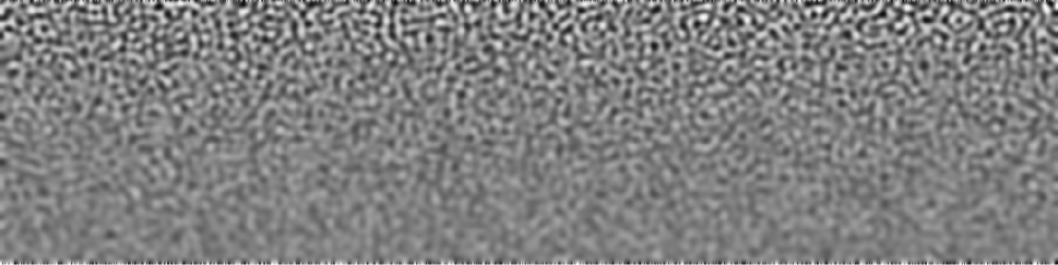
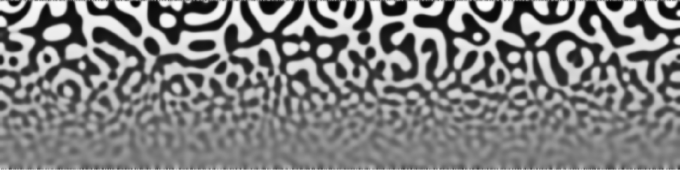
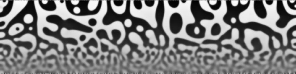
FIG. 5.: Spinodal decomposition of a binary fluid in a rectangular cell of dimensions $a=800$ and $b=200$ (vertical direction in the figures, corresponding to the $y$-direction in the fluid). The parameters used are $C=1,\tau_{0}=1$ and $\alpha=-0.004$. Note that the hotter end is at the bottom of each figure. Shown is the value of the order parameter in grey scale at three instants of time (from top to bottom): $t=6.25,50$ and 100.

REFERENCES

- [1] P. C. Hohenberg and B. I. Halperin, “Theory of dynamic critical phenomena”, Rev. Mod. Phys. 49, 435 (1977).
- [2] E. D. Siggia, B. I. Halperin, and P. C. Hohenberg, “Renormalization-group treatment of the critical dynamics of the binary-fluid and gas-liquid transitions”, Phys. Rev. B 13, 2110 (1976).
- [3] A. Onuki and K. Kawasaki, “Nonequilibrium Steady State of Critical Fluids under Shear Flow: A Renormalization Group Approach”, Ann. Phys. 121, 456 (1979).
- [4] A. Onuki, K. Yamazaki, and K. Kawasaki, “Light scattering by critical fluids under shear flow”, Ann. Phys. 131, 217 (1981).
- [5] E. Helfand and G. H. Fredrickson, “Large fluctuations in polymer solutions under shear”, Phys. Rev. Lett. 62, 2468 (1989).
- [6] M. Doi, in Lecture Notes in Physics, edited by A. Onuki and K. Kawasaki (Springer Verlag, Berlin, 1990), Vol. 52, p. 100.
- [7] K. Kawasaki and T. Ohta, “Kinetics of fluctuations for systems undergoing phase transitions - interfacial approach”, Physica A 118, 175 (1983).
- [8] T. Koga and K. Kawasaki, “Spinodal decomposition in binary fluids: Effects of hydrodynamic interactions”, Phys. Rev. A 44, R817 (1991).
- [9] J. D. Gunton, M. San Miguel, and P. S. Sahni, in Kinetics of first order phase transitions, Vol. 8 of Phase Transitions and Critical Phenomena, edited by C. Domb and J. Lebowitz (Academic, London, 1983).
- [10] L. Landau and E. Lifshitz, Statistical Mechanics, Part 1 (Pergamon, New York, 1980).
- [11] H. Stanley, Introduction to Phase Transitions and Critical Phenomena (Oxford University Press, New York, 1971).
- [12] D. Jasnow, “Critical phenomena at inerfaces”, Rep. Prog. in Physics 47, 1059 (1984).
- [13] D. Jasnow, in Renormalization Group Theory of Interfaces, Vol. 10 of Phase Transitions and Critical Phenomena, edited by C. Domb and J. Lebowitz (Academic, London, 1986).
- [14] J. Rowlinson and B. Widom, Molecular Theory of Capillarity (Clarendon Press, Oxford, 1982).
- [15] M. E. Gurtin, D. Polignone, and J. Viñals, “Two-phase binary fluids and immiscible fluids described by an order parameter”, Math. Models and Methods in Appl. Sci. 6, (1996).
- [16] L. K. Antanovskii, “A phase field model of capillarity”, Phys. Fluids 7, 747 (1995).
- [17] J. Langer, in Chance and Matter, Les Houches Summer School, edited by J. V. J. Souletie and R. Stora (North Holland, Amsterdam, 1986).
- [18] G. Caginalp, in Applications of Field Theory to Statistical Mechanics, Vol. 216 of Lecture Notes in Physics, edited by L. Garrido (Springer-Verlag, Berlin, 1985), p. 216.
- [19] G. Caginalp and P. C. Fife, Phys. Rev. B 33, 7792 (1986).
- [20] We ignore for the time being thermal fluctuations and possible renormalizations due to them.
- [21] C. Peskin, “Numerical analysis of blood flow in the heart”, J. Comp. Phys. 25, 220 (1977).
- [22] J. Hyman, “Numerical methods for tracking interfaces”, Physica D 12, 396 (1984).
- [23] C. W. Hirt and B. D. Nichols, “Volume of fluid (vof) method for the dynamics of free boundaries”, J. Comp. Phys. 39, 201 (1981).
- [24] S. O. Unverdi and G. Trygvasson, “A front-tracking method for viscous, incompressible, multi-fluid flows”, J. Comp. Phys. 100, 25 (1992).
- [25] Q. Shi and H. Haj-Hariri, in Proceedings of the 32nd Aerospace Sciences Meeting (AIAA, Washington, 1994), paper AIAA 94-0834.
- [26] In this case one may introduce an entropy functional instead of a free energy functional along the lines described in [27] and [28].
- [27] S.-L. Wang et al., “Thermodynamically-consistent phase-field models for solidification”, Physica D 69, 189, (1993).
- [28] H.W. Alt and I. Pawlow, Physica D 59, 389 (1992).
- [29] D. Boyanovsky, D. Jasnow, J. Llambías, and S. Takakura, “Statics and dynamics of an interface in a temperature gradient”, Phys. Rev. E 51, 5453 (1995).
- [30] P. Bjorstad et al., Elliptic Problem Solvers II (Academic Press, New York, 1984).
- [31] R. Chella and J. Viñals, “Mixing of a two-phase fluid by cavity flow”, Phys. Rev. E, in press.
- [32] N. Young, J. Goldstein, and J. Block, “The motion of bubbles in a vertical temperature gradient”, J. Fluid Mech. 6, 350 (1959).
- [33] R. S. Subramanian, in Transport Processes in Bubbles, Drops and Particles, edited by R. P. Chhabraand and D. DeKee (Hemisphere Pub. Corp., Washington, D.C., 1990), pp. 1–42.
- [34] Note that one can show for Model H, by using similar arguments as in deriving the tangential and normal surface forces in Section II above, that for weak temperature gradients the velocity is proportional to both the gradient and the radius, independent of the spatial dimensionality.
- [35] J. Llambías, A. Shinozaki, and D. Jasnow, in Proceedings of the Second Microgravity Fluid Physics Conference (NASA, Cleveland, 1994), pp. 207–212, NASA Conference Publication 3276.
- [36] V. Zakharov, V. L’vov, and G. Falkovich, Kolmogorov Spectra of Turbulence I (Springer Verlag, New York, 1992), Chap. 1.
- [37] J. Serrin, in Mathematical Principles of Classical Fluid Mechanics, Vol. VIII/1 of Encyclopedia of Physics, edited by S. Flügge (Springer Verlag, Berlin, 1959), pp. 125–263, section 14-15.
- [38] B. Felderhof, “Dynamics near the diffuse gas-liquid interface near the critical point”, Physica 48, 541 (1970).
- [39] L. Landau and E. Lifshitz, Fluid Mechanics (Pergamon, New York, 1959).