[

Controlling domain patterns far from equilibrium

Abstract

A high degree of control over the structure and dynamics of domain patterns in nonequilibrium systems can be achieved by applying nonuniform external fields near parity breaking front bifurcations. An external field with a linear spatial profile stabilizes a propagating front at a fixed position or induces oscillations with frequency that scales like the square root of the field gradient. Nonmonotonic profiles produce a variety of patterns with controllable wavelengths, domain sizes, and frequencies and phases of oscillations.

]

Technological applications of pattern forming systems are largely unexplored. The few applications that have been pursued, however, have had enormous technological impacts. Magnetic domain patterns in memory devices provide an excellent example [1]. Intensive research effort has been devoted recently to dissipative systems held far from thermal equilibrium [2]. Unlike magnetic materials, such systems are nongradient in general and their asymptotic behaviors need not be stationary; a variety of dynamical behaviors can be realized, including planar and circular traveling waves, rotating spiral waves, breathing structures and spatiotemporal chaos. This wealth of behaviors opens up new opportunities for potential technological applications. Their realizations, however, depend on the ability to control spatiotemporal patterns by weak external forces. Most studies in this direction have focused on drifting localized structures [3].

In this paper we present a novel way to control domain patterns far from equilibrium. We consider dissipative systems exhibiting parity breaking front bifurcations (also referred to as nonequilibrium Ising-Bloch or NIB transitions [4,5]), in which stationary fronts lose stability to pairs of counterpropagating fronts. Examples of systems exhibiting NIB bifurcations include liquid crystals [6] and anisotropic ferromagnets [7] subjected to rotating magnetic fields, chains of coupled electrical oscillators [8], the catalytic CO oxidation on a platinum surface [9,10], the ferrocyanide-iodate-sulphite (FIS) reaction [11], and semiconductor etalons [12]. A prominent feature of these systems is that transitions between the parity broken states, the left and right propagating fronts, become feasible as the front bifurcation is approached. Indeed, intrinsic disturbances, like front curvature and front interactions, are sufficient to induce spontaneous transitions and can lead to complex pattern formation phenomena such as breathing labyrinths, spot replication [11,13] and spiral turbulence [14]. It is this dynamical flexibility near NIB bifurcations that we wish to exploit. By forcing transitions between the left and right propagating fronts, using spatially dependent external fields, we propose to obtain a high degree of control on pattern behavior.

We demonstrate this idea using a forced activator-inhibitor system of the form

$$u_{t} = \epsilon^{-1}(u-u^{3}-v)+u_{xx},$$ (1)

$$v_{t} = u-a_{1}v+\delta v_{xx}+h+Jv_{x},$$ ()

where $u$, the activator, and $v$, the inhibitor, are scalar real fields, and $h$ and $J$ are external fields. With appropriate choice of $a_{1}>0$, the system (1) has two linearly stable stationary uniform solutions, an ”up” state $(u_{+},v_{+})$ and a ”down” state $(u_{-},v_{-})$, and front solutions connecting these states. The domain patterns to be considered here consist of one dimensional arrays of up state regions separated by down state regions. In the absence of the external fields, a stationary front solution, stable for $\epsilon>\epsilon_{c}(\delta)$, loses stability in a pitchfork bifurcation to a pair of fronts propagating in opposite directions at constant speed. For $\epsilon/\delta\ll 1$ the bifurcation point is given by $\epsilon_{c}={9\over 8q^{6}\delta}$ where $q^{2}=a_{1}+1/2$ [14]. Activator inhibitor models have been used to describe some of the systems mentioned above [8,9,10,12]. In these systems $h$ is usually a parameter that introduces an asymmetry between the up and down states. In the context of chemical reactions involving ionic species $J$ may stand for an electric field [15].

FIG. 1.: Front velocity vs. external field, $J$, near the nonequilibrium Ising- Bloch bifurcation. Parameters: $a_{1}=3.0,~{}\epsilon=0.01,~{}\delta=2.0,~{}h=0$.

Consider first the effect of a constant external field on the front velocity. Away from a front bifurcation the effect of a weak field is captured well by a linear approximation and therefore the effect of the field is small. This is not the case close to a front bifurcation; the velocity - external field relation becomes multivalued (or hysteretic) even for a weak field as illustrated in Fig. 1 [8,10,13,16]. This form is a generic unfolding of a pitchfork bifurcation and holds for various unfolding forces and parameters including intrinsic disturbances like curvature [13]. We emphasize that the termination points, $J_{1}$ and $J_{2}$, of the upper and lower branches lie close to $J=0$. The significance is that weak external fields can induce transitions between the two branches, or reverse the direction of front propagation.

The effect of a nonuniform external field [17] can be understood intuitively in the following way. Consider a constant $h$ and a linear profile for $J$: $J=-\alpha x$, where $0<\alpha\ll 1$. This choice divides space into three regions according to the type and number of existing front solutions: (i) $x>x_{1}=-J_{1}/\alpha$, where $J<J_{1}$ and only a single front corresponding to a down state invading an up state exists, (ii) $x<x_{2}=-J_{2}/\alpha$, where $J>J_{2}$ and only a single front corresponding to an up state invading a down state exists, and (iii) $x_{2}<x<x_{1}$, where $J_{1}<J<J_{2}$ and both fronts coexist. This profile of $J$ results in an oscillating front, with oscillations roughly spanning the interval $x_{2}<x<x_{1}$. The front propagation direction is reversed during transitions from the upper to the lower velocity branch at $J\approx J_{1}$ and from the lower to the upper branch at $J\approx J_{2}$. Obviously, a variety of pattern behaviors can be induced using a nonmonotonic $J$ profile. For example, a single hump profile can induce a breathing domain.

We now turn to a quantitative study of front dynamics and relate pattern characteristics (e.g. breathing frequency) to control parameters. We assume $\epsilon\ll 1$ and distinguish between an inner region, the narrow front region, $x\approx x_{f}$, where $u$ varies sharply over a distance of ${\cal O}(\sqrt{\epsilon})$, and outer regions, $x<x_{f}$ and $x>x_{f}$, where $u$ varies on the same scale as $v$.

Consider first the inner region. Expressing (1) in a frame moving with the front, $x\to r=x-x_{f}(t)$, stretching the spatial coordinate according to $z=r/\sqrt{\epsilon}$, and expanding $u=u_{0}+\sqrt{\epsilon}u_{1}+\epsilon u_{2}+...$, $~{}~{}v=v_{0}+\sqrt{\epsilon}v_{1}+\epsilon v_{2}+...$, we find at order unity the stationary front solution, $u_{0}=-\tanh(z/\sqrt{2}),~{}~{}~{}v_{0}=0$. At order $\sqrt{\epsilon}$ we find

$${\cal L}u_{1}=v_{1}-\dot{x}_{f}u_{0z},\qquad{\cal L}=\partial_{z}^{2}+1-3u_{0}^{2}.$$

Solvability of (2) gives

$$\dot{y}_{f}=-{3\over\eta\sqrt{2}}v_{f}(t),$$

up to corrections of ${\cal O}(\epsilon)$, where $y_{f}=x_{f}/\sqrt{\delta}$, $\eta^{2}=\epsilon\delta$, and $v_{f}(t)=v(0,t)$ is the yet undetermined value of the inhibitor at the front position $r=0$.

A dynamical equation for $v_{f}$ follows from an analysis of the outer regions. First we go back to the unstretched coordinate system and rescale the spatial coordinate according to $y=r/\sqrt{\delta}$. At order unity we find

$$v_{t}-\dot{y}_{f}v_{y}=u_{+}(v)-a_{1}v+v_{yy}-\alpha(y+y_{f})v_{y}+h\qquad y\leq 0,$$

and a similar equation for $y\geq 0$ with $u_{+}(v)$ replaced by $u_{-}(v)$. Here $u_{\pm}(v)$ are the outer solution branches of the cubic equation $u-u^{3}-v=0$. In ($4$) we assumed the field $h$ is constant and took a linear profile $J=-\alpha x$. For $a_{1}$ sufficiently large we may linearize the branches $u_{\pm}(v)$ around $v=0$, $u_{\pm}(v)\approx\pm 1-v/2$. Inserting (3) in (4) and using the approximate forms for $u_{\pm}(v)$ we find the free boundary problem

$${\cal M}v = +1-\alpha(y+y_{f})v_{y}+h-{3\over\eta\sqrt{2}}v(0,t)v_{y}\qquad y\leq 0$$ (2)

$${\cal M}v = -1-\alpha(y+y_{f})v_{y}+h-{3\over\eta\sqrt{2}}v(0,t)v_{y}\qquad y\geq 0,$$ (3)

$$v(\pm\infty,t)=v_{\mp}=\mp q^{-2}\qquad\bigl{[}v\bigr{]}_{y=0}=\bigl{[}v_{y}\bigr{]}_{y=0}=0,$$

where ${\cal M}=\partial_{t}+q^{2}-\partial_{x}^{2}$, the square brackets denote jumps across the free boundary at $y=0$, and $v(0,t)$ and $y_{f}(t)$ satisfy (3).

To solve the free boundary problem (5) we assume the system is close to the front bifurcation so that the speed, $c$, of the propagating solutions in the absence of the external fields is small. We also take the external fields to be of order $c^{3}$: $\alpha=\alpha_{0}c^{3}$, $h=h_{0}c^{3}$. We now expand the propagating solutions as a power series in $c$:

$$v(y,t,T)=v^{(0)}(y)+\sum_{n=1}^{\infty}c^{n}v^{(n)}(y,t,T),$$

where $v^{(0)}(y)$, the stationary front solution, is an odd function given by $v^{(0)}(y)=q^{-2}(e^{-qy}-1)$ for $y\geq 0$, and $T=c^{2}t$ is a slow time scale characterizing the nonsteady front motion near the bifurcation. Expanding $\eta$ as well, $\eta=\eta_{c}-c^{2}\eta_{1}+c^{4}\eta_{2}+...,~{}$ and inserting these expansions in (5) we find

$$v^{(n)}_{t}+q^{2}v^{(n)}-v^{(n)}_{yy}=-\rho^{(n)}\qquad n=1,2,3,$$

where

$$\rho^{(1)} = {3\over\sqrt{2}\eta_{c}}v^{(1)}_{|y=0}v^{(0)}_{y},$$ (4)

$$\rho^{(2)} = {3\over\sqrt{2}\eta_{c}}\left[v^{(1)}_{|y=0}v^{(1)}_{y}+v^{(2)}_{|y=0}v^{(0)}_{y}\right],$$ (5)

$$\rho^{(3)} = v^{(1)}_{T}+{3\eta_{1}\over\sqrt{2}\eta_{c}^{2}}v^{(1)}_{|y=0}v^{(0)}_{y}$$ ()

$$+{3\over\sqrt{2}\eta_{c}}\left[v^{(1)}_{|y=0}v^{(2)}_{y}+v^{(2)}_{|y=0}v^{(1)}_{y}+v^{(3)}_{|y=0}v^{(0)}_{y}\right]$$

$$+\alpha_{0}(y+y_{f})v^{(0)}_{y}-h_{0}.$$

The solution of (7) with a zero initial condition (only relevant as long as the long fast time asymptotics is concerned) satisfies the integral equation

$$v^{(n)}(y,t,T) = -\int_{0}^{t}d\tau~{}{e^{-q^{2}(t-\tau)}\over 2[\pi(t-\tau)]^{1/2}}$$ (8)

$$\times\int_{-\infty}^{\infty}d\xi~{}exp\left(-{(y-\xi)^{2}\over 4(t-\tau)}\right)\rho^{(n)}(\xi,\tau,T).$$

Recall that $\rho^{(n)}$ contains the unknown $v^{(n)}$ evaluated at $y=0$. Since the origin of the slow time scale is the nonsteady front motion we expect $v^{(n)}_{|y=0}$ to become independent of the fast time scale $t$ as $t\to\infty$. Substituting $\lim_{t\to\infty}v^{(n)}(0,t,T)=v^{(n)}(0,T)$ in (9) and setting $y=0$ we find a sequence of compatibility conditions. The first, for $n=1$, is $\eta_{c}={3\over 2\sqrt{2}q^{3}}$. The critical value $\eta_{c}=\eta(c=0)$ determines the front bifurcation point. The compatibility condition for $n=3$ is

$$v^{(1)}_{T}(0,T) = {\sqrt{2}\eta_{1}\over q\eta_{c}^{2}}v^{(1)}(0,T)-{3\over 4\eta_{c}^{2}}{v^{(1)}}(0,T)^{3}$$ ()

$$+{2\over 3q}\alpha_{0}y_{f}+{4\over 3}h_{0},$$

where $\eta_{1}={q\eta_{c}^{2}\over 6\sqrt{2}\delta}$. Expressing (10) in terms of $v_{f}=v(0,T)\approx cv^{(1)}(0,T)$ and using $c^{2}\eta_{1}\approx\eta_{c}-\eta$ we find

$$\dot{v}_{f}={\sqrt{2}\over q\eta_{c}^{2}}(\eta_{c}-\eta)v_{f}-{3\over 4\eta_{c}^{2}}v_{f}^{3}+{2\over 3q}\alpha y_{f}+{4\over 3}h,$$ (10)

where $\dot{v}_{f}=c^{2}{v_{f}}_{T}$.

Equations (3) and (11) describe the dynamics of fronts near a NIB bifurcation, subjected to a constant field $h$ and a linearly space dependent $J$ field. In addition to the translational degree of freedom, $y_{f}$, the dynamics involve a second degree of freedom, the value of the inhibitor at the front position, $v_{f}$, which is responsible for transitions between the left and right propagating fronts. Without the field $J$ the system (3) and (11) is decoupled and reproduces the front bifurcation. The introduction of a space dependent field couples the two degrees of freedom and affects the front behavior in two significant ways: for $\eta>\eta_{c}$ (and $h\neq 0$) it stabilizes a propagating front at a fixed position, $y_{f}=-{2qh\over\alpha}$, and for $\eta<\eta_{c}$ it induces oscillations between the counterpropagating fronts. The frequency of oscillations close to the Hopf bifurcation at $\eta=\eta_{c}$ is

$$\omega={2\over\sqrt{3}}q\sqrt{\alpha}.$$

FIG. 2.: (a) Front position, $x_{f}$, vs. time for an oscillating front. The thin line represents the solution to equations (3) and (11) and the diamonds are from the numerical solution of equations (1). (b) A log-log plot of the oscillation frequency, $\omega$, vs. the external field gradient, $\alpha$. The solid line is the relation of equation (12) and the diamonds represent numerical solutions of equations (1). Parameters: $a_{1}=3.0,~{}\epsilon=0.01,~{}\delta=2.77,~{}h=0$ and $\alpha=0.005$ in (a).

To test the validity of equations (3) and (11) we numerically integrated the original system (1) and compared oscillating front solutions of (1) with those of (3) and (11). The agreement as Fig. 2$a$ shows is very good. In Fig. 2$b$ we plotted the frequency of front oscillations vs. the field gradient according to (12) and as obtained from (1). Again, the agreement is excellent, and remains good even for $c$ of order unity.

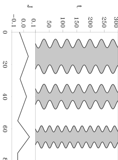
FIG. 3.: The oscillating domain on the left has the same frequency as middle domain but the wider separation between the $J=0$ points produces a larger domain size. The domain on the right has the same average width as the middle domain but the larger external field gradient produces higher frequency. Parameters: $a_{1}=3.0,~{}\epsilon=0.01,~{}\delta=2.77,~{}h=0$.

These results suggest various ways to control domain patterns.

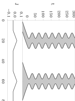
FIG. 4.: The phase of oscillation is determined by the $v_{f}$ values of the fronts that bound a domain. Opposite signs of $v_{f}$ give rise to a traveling domain that oscillates back and forth (left domain). Equal signs of $v_{f}$ yield a breathing domain (right domain). Parameters: $a_{1}=3.0,~{}\epsilon=0.01,~{}\delta=2.77,~{}h=0$.

Choosing a periodic $J(x)$ profile, for example, allows the creation of a periodic pattern of stationary ($\eta>\eta_{c}$) or oscillating ($\eta<\eta_{c}$) domains. The period of the pattern, the average width of the domains, and the frequency and relative phase of oscillations are easily controllable. Figs. 3 and 4 show the effect of a nonuniform triangular profile of $J$ for $\eta<\eta_{c}$. In the absence of $J$ the system supports traveling domain patterns. Switching on $J(x)$ gives rise to patterns of oscillating domains. Regions of $J(x)$ where the gradient $\alpha(x)=|J^{\prime}(x)|$ is steeper yield higher oscillation frequencies in accord with (12), while wider $J$ triangles yield wider domains (Fig. 3). The relative phase of oscillation is controlled by the values of $v_{f}$ for the two fronts that bound a domain. Choosing the same sign for $v_{f}$ gives rise to breathing dynamics whereas opposite signs yield back and forth oscillations (Fig. 4). For $\eta>\eta_{c}$ arbitrary stationary domain patterns can be formed with appropriate $J(x)$ profiles; the only restriction is the requirement of a minimum domain size to guarantee the dominance of $J$ over front interactions. Similar results are obtained with a nonuniform $h$ field and constant $J$. We expect the main ideas presented here to apply to other models exhibiting NIB bifurcations, such as the forced complex Ginzburg-Landau equation [4].

REFERENCES

- [1] E.D. Dahlberg and J.-G. Zhu, Physics Today 48(4), 34 (1995).
- [2] M.C. Cross and P.C. Hohenberg, Rev. Mod. Phys. 65, 2 (1993).
- [3] V.S. Zykov, O. Steinbock, and S.C. Müller, Chaos 4, 509 (1994), and references therein.
- [4] P. Coullet, J. Lega, B. Houchmanzadeh, and J. Lajzerowicz, Phys. Rev. Lett. 65, 1352 (1990).
- [5] A. Hagberg and E. Meron, Nonlinearity 7, 805 (1994).
- [6] T. Frisch, S. Rica, P. Coullet, and J.M. Gilli, Phys. Rev. Lett. 72, 1471 (1994); K.B. Migler and R.B. Meyer, Physica D 71, 412 (1994); S. Nasuno, N. Yoshimo, and S. Kai, Phys. Rev. E 51, 1598 (1995).
- [7] P. Coullet, J. Lega, and Y. Pomeau, Europhys. Lett. 15, 221 (1991).
- [8] M. Bode, A. Reuter, R. Schmeling, and H.-G. Purwins, Phys. Lett. A 185, 70 (1994).
- [9] M. Bär, S. Nettesheim, H.H. Rotermund, M. Eiswirth, and G. Ertl, Phys. Rev. Lett. 74, 1246 (1995).
- [10] G. Haas, M. Bär, I.G. Kevrekidis, P.B. Rasmussen, H.-H. Rotermund and G. Ertl, Phys. Rev. Lett. 75, 3560 (1995).
- [11] K.J. Lee, W.D. McCormick, H.L. Swinney, and J.E. Pearson, Nature 369, 215 (1994); K.J. Lee and H.L. Swinney, Phys. Rev. E 51, 1899 (1995).
- [12] Y.A. Rzhanov, H. Richardson, A.A. Hagberg and J. Moloney, Phys. Rev. A 47, 1480 (1993).
- [13] C. Elphick, A. Hagberg, and E. Meron, Phys. Rev. E 51 (1995) 3052.
- [14] A. Hagberg and E. Meron, Phys. Rev. Lett. 72, 2494 (1994); A. Hagberg and E. Meron, Chaos 4 (1994) 477.
- [15] O. Steinbock, J. Schütze, and S.C. Müller, Phys. Rev. Lett. 68, 248 (1992); J.J. Taboada, A.P. Muñuzuri, V. Pérez-Muñuzuri, M. Gómez-Gesteira, and V. Pérez-Villar, Chaos 4, 519 (1994).
- [16] P. Ortoleva, Physica 26D, 67 (1987).
- [17] P. Schütz, M. Bode, and Hans-Georg Purwins, Physica D 82 (1995) 382.