Front Stability in Mean Field Models of Diffusion Limited Growth

Abstract

We present calculations of the stability of planar fronts in two mean field models of diffusion limited growth. The steady state solution for the front can exist for a continuous family of velocities, we show that the selected velocity is given by marginal stability theory. We find that naive mean field theory has no instability to transverse perturbations, while a threshold mean field theory has such a Mullins-Sekerka instability. These results place on firm theoretical ground the observed lack of the dendritic morphology in naive mean field theory and its presence in threshold models. The existence of a Mullins-Sekerka instability is related to the behavior of the mean field theories in the zero-undercooling limit.

I Introduction

Some of the most appealing and difficult patterns found in nature are formed by diffusion limited growth. A canonical example is solidification patterns [1, 2], which, in addition to generating the delicate beauty of snowflakes, are important metallurgically as the source of alloy microstructure. Diffusion limited growth drives pattern formation in a wide variety of systems: examples include fingering patterns in the displacement of a viscous fluid [1], electrodeposition patterns [3, 4], microbial aggregation [5, 6], dielectric breakdown, flow in oil reservoirs, and possibly the wiring of neuronal dendritic arbors [7].

In recent years, much progress has been made on the problem of constructing a theory of pattern formation in dissipative systems [8]. This theory explains the universal patterns seen in systems where a linear instability of a uniform ground state saturates at some finite amplitude. In this context, diffusion limited growth patterns form an interesting example of a pattern forming system whose instability never saturates.

The instability which drives pattern formation in diffusion limited growth is the Mullins-Sekerka instability. The physical nature of this instability can be seen by considering a solid seed particle immersed in a supercooled liquid bath. As the liquid solidifies around the seed, the latent heat released by the first order phase transition must diffuse away. An outward perturbation on the boundary of the growing solid can cool more easily, and so grows faster than neighboring regions, leading to an instability of the solid-liquid interface. Competition between the Mullins-Sekerka instability and other effects, such as surface tension, sets a basic length scale for pattern formation. As boundary features formed by the Mullins-Sekerka instability eventually grow to a size where they too are unstable, new structures grow on them, and highly complex fractal patterns are formed.

Diffusion limited growth occurs in at least two broad morphologies: tip splitting growth, as seen for example in Hele-Shaw flow in a radial geometry, and dendritic growth, as observed in solidification. In a radial geometry, tip splitting growth forms branching fingers whose ensemble averaged envelope is circular, while dendritic growth forms a concave envelope lead by cusp-like tips propagating at some fixed velocity. The mechanism acting at the tips to select the actual behavior is understood: anisotropy in the surface tension (or phase transformation kinetics) acts as a singular perturbation at the tip to stabilize the dendrite, with the unique velocity being selected by a microscopic solvability condition [1]. If anisotropy is absent, no propagating dendrite can be formed, and tip splitting growth is observed.

More recent work is on global aspects of these pattern forming systems. There is numerical evidence [9, 10, 11] for a morphology transition between the concave asymptotic profiles of the dendritic growth morphology and the convex asymptotic profiles of the densely branched morphology (DBM). The work of Shochet et al. suggests that there is a discontinuity in the slope of the velocity vs. control parameter curve at the convex to concave transition, implying that the different morphologies are akin to thermodynamically different states. This kinetic phase transition hypothesis is bolstered by their suggestion that there may be coexistence between the branching and dendritic morphologies [12].

One step towards theoretical understanding of this morphology transition and of diffusion growth patterns in general is to formulate an envelope model which displays the convex/concave transition of the underlying microscopic models. Such a model, based on the classic mean field models of Witten and Sander [13], has been proposed [14, 15, 16, 17]. Since a model for the envelope cannot allow concavity (or the dendritic morphology) if it forms stable planar fronts (by the kinetic Wulff construction discussed in Section III), it is necessary to look for a Mullins-Sekerka instability in the models discussed in [17], and to understand the nature of that instability.

In the remainder of this paper we will discuss several microscopic solidification models in general and review the behaviors of the mean field models (Section II). We will present some background on the geometrical construction of asymptotic shapes (Section III), the relationship between morphology transitions and the Mullins-Sekerka instability, and the velocity selection of planar fronts (Section III A). Our calculation of the stability of planar fronts in mean field models will be presented in Section IV A. The zero undercooling limit will be discussed in Section V, and our conclusions appear in Section VI.

II Models and Mean Field Theory

Modelling efforts for diffusion limited growth have taken a variety of forms. The direct continuum approach for a sharp interface is in terms of a moving boundary value problem [1]. The field controlling growth ($u$, which is proportional to the undercooling $T_{m}-T$) satisfies the diffusion equation

$$\partial_{t}u=D\nabla^{2}u\mbox{ .}$$ (1)

The boundary conditions are undercooling at infinity and a melting point on the boundary set by a surface tension $\gamma$ (due to the Gibbs-Thompson condition) and phase transformation kinetics

$$\begin{array}[]{rcl}u|_{+\infty}&=&\Delta\\ u|_{\mbox{interface}}&=&-\gamma\kappa-\beta v_{n}\mbox{ .}\end{array}$$ (2)

The boundary motion is determined by the local gradient of the diffusing field

$$v_{n}=\nabla u|_{\mbox{interface}}\cdot\hat{n}$$ (3)

where $\hat{n}$ is the normal unit vector of the interface. The displacement of a more viscous fluid by a less viscous fluid (the Saffman-Taylor problem) or flow in porous media satisfies similar equations, with the field $u$ representing pressure in the fluid[1].

More flexibility is offered by phase field models, which specify a continuous transition from the solid to liquid phase [18, 19, 20], allowing arbitrary topology of the interface and more control over the boundary layer and the phase transformation at the expense of an additional field.

Another approach is the diffusion limited aggregation (DLA) class of models [13, 21], which have generated a great deal of interest. This approach models diffusion limited growth by the discrete aggregation of random walkers, with the probability density of a random walk capturing diffusive behavior in a computationally efficient scheme. The random fractal nature of these aggregates motivate questions about the effects of noise. A phase field model with stochastic properties is studied in [22]. Other models include the cell dynamical scheme [23] and the diffusion transition scheme [10], both of which couple numerical solution of the diffusive field with some model for the phase transition in cells on a lattice. Noise is an inherent part of these models as well.

The various different growth morphologies may all be observed within any particular model, depending on such parameters as boundary conditions, undercooling, surface tension, kinetic effect, anisotropy, etc. The dendritic morphology occurs at finite anisotropy, finite undercooling; while single walker DLA corresponds to zero undercooling, zero surface tension and kinetic effect. Tip splitting growth as seen in radial Hele-Shaw flow and Saffman-Taylor fingers in a channel geometry occurs at zero anisotropy.

A Mean field theory

Mean field models attempt to capture global morphology of diffusion limited growth. Naive mean field theory in open radial geometries at zero undercooling has a spherically symmetric solution which captures the mass scaling behavior of single walker DLA, giving a mean field exponent of $d_{f}=d-1$, a number believed to become exact as $d\rightarrow\infty$. However, this spherically symmetric solution is always unstable, leading to difficulties of interpretation. In addition, the naive mean field theory fails in one dimension or in a channel geometry, where fronts accelerate to infinite velocity in finite time [14]. A phenomenological modification of the naive MFT has been proposed which fixes these problems and successfully explains several important morphological observations. One is that the envelope of ensemble averages of DLA in a channel geometry takes the shape of a Saffman-Taylor finger [14], and another is that anisotropic growth in a radial geometry can form the global dendritic morphology [17]. There are now indications that the necessary threshold suggested phenomenologically in [14] can be generated by including the essential effects of noise in underlying model [24].

We begin our discussion of mean field theory by considering the Witten-Sander aggregation model with finite walker density. In this model, the diffusion field controlling growth is modelled by random walkers. When a walker becomes adjacent to the solid, it transforms into solid and advances the solid to that position. This sticking rule implies that the walker density $u$ on the boundary is zero, giving a walker density adjacent to the boundary of $a\nabla u$. This gives a growth velocity proportional to $\nabla u$. Comparison with (2) and (3) shows that DLA is a stochastic model for diffusion limited interface growth with no surface tension or interface kinetics. The random walker density will satisfy the diffusion equation, minus the walkers lost to the growing aggregate density $\rho$

$$\dot{u}=D\nabla^{2}u-\dot{\rho}\mbox{ .}$$ (4)

The transition probability of an unoccupied site ${\bf x}$ is proportional to

$$u{\bf(x},t)P({\bf x},t)$$ (5)

where $P({\bf x})$ represent the probability of the neighboring sites to be occupied by the aggregate. We can write $P({\bf x})$ in the form

$$P({\bf x})=\sum_{i}\rho({\bf x}+{\bf e}_{i})$$ (6)

where ${\bf e}_{i}$ are lattice vectors to adjacent sites and $i$ runs over the number of nearest neighbors. This formulation allows multiple walkers to occupy a single site, a feature not expected to affect the universality class.

We derive a continuum mean field model by allowing $u$ and $\rho$ to take on any continuum values and identifying the sum of nearest neighbor terms in $P$ as a lattice Laplacian. This results in the Witten-Sander mean field model for finite walker density DLA:

$$\dot{u} = D\nabla^{2}u-\dot{\rho}$$ (7)

$$\dot{\rho} = Ku(\rho+a^{2}\nabla^{2}\rho)\mbox{ .}$$ (8)

where the constant parameters $D$, $K$ and $a$ can be removed by setting $x\rightarrow{ax}$, $t\rightarrow ta^{2}/D$, and $\{\rho,u\}\rightarrow\{\rho,u\}D/a^{2}K$. In these units the equations become

$$\dot{u} = \nabla^{2}u-\dot{\rho}$$ (9)

$$\dot{\rho} = u(\rho+\nabla^{2}\rho)$$ (10)

with a boundary condition on the undercooling, or walker density at infinity $u|_{+\infty}=\Delta$. The total number of particles (aggregated and walking) $\rho+u$ is conserved by the local dynamics.

This mean field theory has no threshold for aggregate growth, so a small perturbation in the $\rho$ field, in the presence of $u$, will grow exponentially. However, lattice simulations with discrete phase states, including the DLA model discussed above as well as others [23, 13, 10], have an implicit threshold for growth: growth at a site is disallowed unless a nearest neighbor site is fully occupied. Phase field models also have a threshold, in this case explicit in the structure of the form of the free energy, which specifies that the phases are at least metastable [22, 18]. This lack of a threshold in naive MFT leads to problems in channel or planar geometries, namely the infinite propagation mentioned earlier. Inserting a threshold by hand, we have the phenomenological model introduced by Brener et al.  [14]:

$$\begin{array}[]{rcl}\dot{u}&=&\nabla^{2}u-\dot{\rho}\\ \dot{\rho}&=&u(\rho^{\gamma}+\nabla^{2}\rho)\mbox{ .}\end{array}$$ (11)

Any function $F(\rho)$ which vanishes faster than linearly as $\rho\rightarrow 0$ could be used in the place of $\rho^{\gamma}$, for example $F(\rho)=\rho\Theta(\rho-A)$.

The success of the $\gamma$ model motivates the question of how to obtain such a growth threshold in a more fundamental way. One possibility is to invoke the generic effects of noise [24]. In microscopic theory, thermal noise at the tip drives sidebranching [1]. In the Witten-Sander particle aggregation model, shot noise of particle diffusion and aggregation are a source of noise. Noise is known to shift the bifurcation point of nonlinear systems [25, 26].

To sketch how noise may affect the form of the macroscopic mean field equations, recall the derivation of the naive mean field theory (7, 8) from the Witten-Sander rules. The transitions of particles on a nearest neighbor site from walker to aggregate are random and independent, and therefore governed by Poissonian shot noise. Including these fluctuations by a Langevin noise source $\eta$ multiplicatively coupled with the field, we have

$$\dot{\rho}=Ku(\rho+a^{2}\nabla^{2}\rho)+\sqrt{Ku(\rho+a^{2}\nabla^{2}\rho)}\ \eta$$ (12)

Multiplicatively coupled noise can lead to stabilization of an unstable system, analogous in some ways to a parametrically driven pendulum [26]. This stabilization is exactly what is required, as it establishes a lower threshold in $\rho$ below which growth does not occur. A more complete discussion appears in [24].

III Theory of kinetic morphology

In this section, we review some material concerning the growth of envelopes. A system with a transition layer that does not spread will in the long time limit be described by a sharp interface model. We parameterize the interface between the two phases by a curve $\vec{x}(\sigma,t)$ and write the evolution of this curve in the form

$${d\vec{x}\over dt}=\vec{v}(\sigma,t,[\vec{x}])$$ (13)

where $\vec{v}$ can in general be a complicated functional depending nonlocally on the entire curve $\vec{x}$. We are interested in envelopes which form a well defined shape in the asymptotic time limit, that is assume a scaling form

$$\vec{x}(\sigma,t)=R(t)\vec{r}(\sigma)\mbox{ .}$$ (14)

Since velocity parallel to the interface corresponds merely to a redefinition of the parameterization $\sigma$, we take $\vec{v}=v_{n}\hat{n}$. From (13) and (14) we get

$${d\vec{x}\over dt}=\dot{R}(t)\vec{r}(\sigma)=v_{n}(\sigma,t)\hat{n}$$ (15)

If the envelope scales, the time dependence will factor out of $v_{n}$, leaving us with

$$v_{n}(\sigma)=\vec{r}(\sigma)\cdot\hat{n}\mbox{ .}$$ (16)

One may imagine several possibilities for the nature of $v_{n}$. For example, in a sharp interface model for diffusion limited growth, $v_{n}$ will depend on the whole structure and history of the envelope in some nonlocal way. Alternatively, it may be that $v$ depends only on purely local properties of the interface, such as the normal direction, curvature and so on. In the asymptotic limit, the envelope locally appears to be flat, leaving the normal direction as the only remaining variable that $v$ can depend on. In this case, one can solve for the envelope shape explicitly given $v_{n}(\hat{n})$ for all angles of flat front propagation. This is done by the kinetic Wulff construction to be discussed next.

The equilibrium shape of a crystal has a solution in the form of the Wulff construction which dates back to the turn of the century [27, 28]. Given the anisotropic form of the surface energy $\gamma(\theta)$ for each crystal direction $\theta$, minimizing the total surface energy (at fixed area) leads to the following construction: for every normal direction, draw a line perpendicular to the normal at a distance from the origin proportional to surface energy of that direction. The inner convex hull of these lines is the equilibrium crystal shape. The resulting crystal may be faceted, smooth (if it is above the roughening transition) or may have both facets and smoothly curved surfaces.

If a crystal is grown under such conditions that the normal velocity depends only on the direction of the surface normal (for example, in a reaction limited regime), then the steady state shape is again given by the Wulff construction, with normal velocity substituted in for surface energy. It is clear that such a steady state cannot be concave [29, 30]. Because the envelope of the dendritic morphology is concave [11], a geometrical model cannot capture the dendritic morphology.

Although the kinetic Wulff construction is not applicable to the nonlocal diffusion limited regime, it is important to understand its consequences for general modelling of the morphology transition. A model which forms stable planar fronts at any angle in two dimensions cannot capture the dendritic morphology. In the asymptotic limit, a scaling form will arise, composed of approximately planar fronts. The velocities of these planar fronts as a function of angle can be found by marginal stability. The asymptotic shape will therefore be given by the kinetic Wulff construction, and will be convex. So a mean field theory which always has a stable planar front cannot model the dendritic (concave) morphology, and cannot describe the morphology transition. In fact, in the convex regime, the planar front has to have an instability analogous to Mullins-Sekerka instabilty. It is for this reason that we have tested for the presence of a Mullins-Sekerka instability in mean field models.

In our calculations we have not included a term such as

$$\epsilon\left[\frac{\partial^{4}\rho}{\partial x^{4}}+\frac{\partial^{4}\rho}{\partial y^{4}}\right]$$ (17)

to explicitly include anisotropy. Although such an anisotropy term is of course a necessary ingredient for dendritic growth, we have neglected it for simplicity. Its effect will be small; its function at the level of our linear stability analysis would merely be to pick out a preferred direction for the instability to grow. This point of view is verified in 2d simulations, which show explicitly the existence of dendritic growth in exactly those systems with a Mullins-Sekerka instability in isotropic planar fronts[17].

A Marginal stability

To find the front velocity $v(\theta)$ used above, it is necessary to find the velocities of planar fronts in the desired model. The mean field diffusion growth equations derived earlier have the generic property (shared with other nonlinear diffusion equations) that there exist steady state solutions of any velocity. This property is connected with the unstable nature of the invaded state, so it does not apply to models with a strict cutoff, although it does apply to the $\gamma$ model with its power law cutoff. The first task is therefore the solution of a velocity selection problem. Marginal stability theory states that, for typical initial conditions, the selected velocity is the lowest velocity for which localized perturbations are stable in the moving reference frame[31, 8]. Here, “localized” means perturbations whose asymptotic tails decay no slower than the front itself, and are therefore smaller than the front everywhere. Marginal stability is on a firm foundation for nonlinear diffusion problems with one variable. Marginal stability falls into two classes: linear marginal stability, where computing the stability of the asymptotic tail is sufficient, and nonlinear marginal stability, where the (linear) stability of the entire front needs to be considered. In one variable velocity selection problems, such as the Fisher equation $\dot{u}=u(1-u)+\nabla^{2}u$, a parameter counting argument indicates a continuum of unstable modes in the regime where the front oscillates[31], i.e. where $c<1/2$. In problems involving nonlinear marginal stability, it is the appearance of a discrete unstable mode which sets the marginally stable velocity.

There is a qualitative distinction between fronts selected by linear and nonlinear marginal stability. In either case the front is formed as a balance between the growth of the density and its diffusion which catalyzes further growth. In the linear case, the growth of the front at its leading edge is sufficient to catalyze its continued propagating, in this case we speak of the front being “pulled” by its leading edge. In the nonlinear case, the linear growth rate of the leading edge is insufficient to maintain the propagation velocity, and the larger nonlinear growth in the body of the front is necessary to catalyze the continued propagation. In this case, we speak of the front being “pushed” by the growth behind the front [32].

To compare with the one dimensional marginal stability theory we compute, for the naive ($\gamma=1$) model, the asymptotic behavior of the front at $z=+\infty$. This can be found by setting $u=\Delta$ in the equations for a steady state front (see Section IV) giving

$$-c\rho^{\prime}=\Delta(\rho+\rho^{\prime\prime})\mbox{ .}$$ (18)

This has solutions $\rho\sim\exp{\lambda_{\pm}z}$ where $\lambda_{\pm}$ is given by

$$\lambda_{\pm}=-{c\over{2\Delta}}\pm\sqrt{{c^{2}\over 4\Delta^{2}}-1}\mbox{ .}$$ (19)

For $c<2\Delta$, these modes oscillate, which can be prohibited on physical grounds by the interpretation of $\rho$ as a density. The parameter counting argument analogous to the nonlinear diffusion case is complicated by an additional variable and an additional free parameter ($\Delta$) but the result is the same: namely, that we have a continuum of instabilities in the regime where the fields acquire oscillating tails, predicting a linear marginally stable velocity of $c=2\Delta$.

For $\gamma>1$, we expect similar behavior — the selected velocity will be the slowest stable velocity, which will again be the lowest velocity for which $\rho$ does not cross zero. In this case, however, this will not be given by the behavior of the asymptotic tail. The linear growth rate for $\gamma>1$ is zero, and therefore any front formed must be pushed, with a velocity given by nonlinear marginal stability.

IV Perturbation of moving fronts

We will write out the equations describing perturbations of fronts satisfying (11). We consider a planar geometry, so that the only spatial dependence is $x$ dependence, and we will add transversal dependence back in later. Working in a moving frame $z=x-ct$ and looking for a steady state solution $\rho_{t}=u_{t}=0$ we have

$$-cu^{\prime} = u^{\prime\prime}-c\rho^{\prime}$$ (20)

$$-c\rho^{\prime} = u(F(\rho)+\rho^{\prime\prime})$$ (21)

where primes indicate $z$ derivatives. By integrating and using the boundary conditions $\rho=\Delta$, $u=0$ at $z=-\infty$ the first equation becomes

$$u^{\prime}=c(\Delta-\rho-u)\mbox{ .}$$ (22)

By integrating forward from $z=-\infty$, a steady state front can be found for any desired velocity.

The base solutions may be found by numerically integrating the equations. Initial conditions at the left are chosen to assure the boundary conditions $u\rightarrow 0$ and $\rho\rightarrow\Delta$ as $z\rightarrow-\infty$. Since the $\rho$ field may become negative, we use $\mbox{sgn}(\rho)|\rho|^{\gamma}$ as our threshold function. Next we do perturbation theory on our equations in the moving frame

$$\dot{u}-c\partial_{z}u =\nabla^{2}u-\dot{\rho}+c\partial_{z}\rho$$ (23)

$$\dot{\rho}-c\partial_{z}\rho =u(F(\rho)+\nabla^{2}\rho)$$ (24)

where we include transversal dependence in our perturbation

$$u =u^{0}(z)+e^{\omega t}e^{iky}u^{1}(z)$$ (25)

$$\rho =\rho^{0}(z)+e^{\omega t}e^{iky}\rho^{1}(z)$$ (26)

and look for eigenfunctions $u^{1}$ and $\rho^{1}$ which go to zero as $z\rightarrow\pm\infty$. Linearizing, we get

$$\omega u^{1}-c{u^{1}}^{\prime}=-k^{2}u^{1}+{u^{1}}^{\prime\prime}-\omega\rho^{1}+c{\rho^{1}}^{\prime}$$ (27)

$$\omega\rho^{1}-c{\rho^{1}}^{\prime} = u^{0}(z)(F^{\prime}(\rho^{0}(z))\rho^{1}-k^{2}\rho^{1}+{\rho^{1}}^{\prime\prime})$$ (29)

$$+u^{1}(F(\rho^{0}(z))+{\rho^{0}}^{\prime\prime}(z))$$

Since there is little hope of solving this eigenvalue problem exactly, we discretize it in a box and diagonalize it numerically. To put this in a form which is easy to discretize, we write it as

$$\left[\begin{array}[]{cc}D^{2}+cD-(F(\rho^{0})+{\rho^{0}}^{\prime\prime}+k^{2})&-u^{0}D^{2}-u^{0}(F^{\prime}(\rho^{0})-k^{2})\\ (F(\rho^{0})+{\rho^{0}}^{\prime\prime})&u^{0}D^{2}+cD+u^{0}(F^{\prime}(\rho^{0})-k^{2})\end{array}\right]\left[\begin{array}[]{c}u^{1}\\ \rho^{1}\end{array}\right]=\omega\left[\begin{array}[]{c}u^{1}\\ \rho^{1}\end{array}\right]$$ (30)

where $D$ represents the finite difference approximation of a derivative expressed as a tridiagonal matrix.

Now, we also want our perturbation to decay as fast or faster than the base solution at $z=+\infty$. To do this, we can rewrite our eigenvalue problem in terms of new variables, having divided out the asymptotic fall-off of the base solution tails on the right, after which a zero-slope boundary condition on the right enforces the localized perturbation condition. Explicitly, if we let $u^{1}_{old}=f_{u}(z)u^{1}_{new}$, and $\rho^{1}_{old}=f_{\rho}(z)\rho^{1}_{new}$, where the $f$ functions have the same dependence at large $z$ as the base solution and approach a constant at the left, then we have

$$Du^{1}=Df_{u}(z)u^{1}_{new}=f_{u}(z)(\frac{f^{\prime}_{u}}{f_{u}}+D)u^{1}_{new}$$ (31)

and

$$D^{2}u^{1} =f_{u}(z)(\frac{f^{\prime}_{u}}{f_{u}}+D)^{2}u^{1}_{new}$$ (33)

$$=f_{u}(z)(\frac{f^{\prime\prime}_{u}}{f}+2\frac{f_{u}^{\prime}}{f}D+D^{2})u^{1}_{new}\mbox{ .}$$

Making the replacements $D\rightarrow D+\frac{f^{\prime}}{f}$ and $D^{2}\rightarrow D^{2}+2\frac{f^{\prime}}{f}D+\frac{f^{\prime\prime}}{f}$ in the perturbation equations (30), we have

$$\left[\begin{array}[]{c}D^{2}+(c+2\frac{f_{u}^{\prime}}{f_{u}})D+(-F(\rho^{0})-{\rho^{0}}^{\prime\prime}-k^{2}+\frac{f_{u}^{\prime\prime}}{f_{u}}+c\frac{f_{u}^{\prime}}{f_{u}})\\ \frac{f_{u}}{f_{\rho}}(F(\rho^{0})+{\rho^{0}}^{\prime\prime})\end{array}\right.$$ (36)

$$\left.\begin{array}[]{c}\frac{f_{\rho}}{f_{u}}\{-u^{0}D^{2}-2\frac{f_{\rho}^{\prime}}{f_{\rho}}u^{0}D-u^{0}(F^{\prime}(\rho^{0})-k^{2}+\frac{f_{\rho}^{\prime\prime}}{f_{\rho}})\}\\ u^{0}D^{2}+(c+2\frac{f_{\rho}^{\prime}}{f_{\rho}}u^{0})D+u^{0}(F^{\prime}(\rho^{0})-k^{2}+\frac{f_{\rho}^{\prime\prime}}{f_{\rho}})+c\frac{f_{\rho}^{\prime}}{f_{\rho}}\end{array}\right]\left[\begin{array}[]{c}u^{1}\\ \rho^{1}\end{array}\right]=\omega\left[\begin{array}[]{c}u^{1}\\ \rho^{1}\end{array}\right]$$ (43)

The functions $f$ are computed from the base solution for $\gamma>1$ and chosen analytically for $\gamma=1$. The growth rates of possible perturbations are just the eigenvalues of this nonsymmetric matrix, which can be found numerically by standard techniques.

A Numerical results

We first display the results relating to velocity selection by marginal stability. The behavior of the largest growth rate $\omega_{\rm max}$ near $c_{\rm ms}=2\Delta$ for $\gamma=1$ is shown in Figure 1. As expected, we see that the growth rate for the most unstable mode drops to zero as $c$ passes through $2\Delta$, implying a selected velocity of $2\Delta$. This velocity selection has been verified in direct numerical simulations. At $\gamma=1$, then, the front is pulled, and linear marginal stability holds.

The profiles of the $u$ and $\rho$ fields at a velocity smaller than $c_{\rm ms}$ for $\gamma>1$ are shown in Figure 2. At this velocity, the $\rho$ field crosses zero to become negative. This creates a well allowing a discrete unstable mode, analogous to a bound state in a well in quantum wave mechanics. For $\gamma>1$, we again expect the velocity to be given by the velocity of the slowest stable front. This is now a global stability calculation for the velocity of a pushed front. This velocity selection is verified in Figure 3, which compares the velocity calculated from numerical diagonalization at $\gamma=1.2$ with the velocity as measured in simulations. It is clear that nonlinear marginal stability theory is predicting the correct velocities as measured in simulations, and that the $\gamma$ model gives pushed fronts.

The nature of the instability for $\gamma>1$ is indicated by the spectrum shown in Figure 4. As $c$ passes below $c_{\rm ms}$, a single discrete mode moves above zero. This is in contrast to the $\gamma=1$ case, where the top of a continuum moves above zero, but it is natural in light of the fact that $\rho$ decays as a power law and cannot have the oscillating tail that generates the continuum in the $\gamma=1$ case. Figure 3 shows a quadratic extrapolation to zero velocity, which occurs for $\gamma=1.2$ at $\Delta=\Delta^{*}\simeq 0.055$. This defines $\Delta^{*}$, the lowest undercooling at which the model can form a propagating front. Nonzero $\Delta^{*}$ is the essential feature of threshold mean field theories, and is not found in naive mean field theory, for which (since $c_{\rm ms}=2\Delta$) $\Delta^{*}=0$. The transverse stability calculation is done for the selected planar front, and this calculation gives the required front velocities.

Our main results concern the existence of a Mullins-Sekerka instability [33] in these models. Again we restrict ourselves to perturbations which decay at least as fast as the front. Figure 5 shows the growth rate $\omega$ of the most unstable mode in naive mean field model plotted as a function of the transverse wavenumber $k$ for a number of undercoolings $\Delta$. There is no sign of any finite wavenumber instability.

Figure 6 shows the largest growth rate $\omega$ vs. $k$ for a number of $\Delta$’s in the $\gamma$ model at $\gamma=1.2$. There is a finite $k$ instability for $\Delta$ below $\Delta^{**}\simeq 0.29$. Figure 7 shows a typical unstable spectrum. The characteristic length scale of the instability is comparable to the width of the front. Comparing with Figure 3, note that there is no sign of any velocity slope discontinuity at the point $\Delta^{**}\simeq 0.29$ where the Mullins-Sekerka instability disappears. This argues against the morphology transition being some kind of nonequilibrium phase transition. These results demonstrate explicitly what was already indicated in [17]: a threshold is necessary to generate a Mullins-Sekerka instability and allow concave dendritic envelopes to be formed, and that the $\gamma$ threshold model in particular both has concave envelopes and a Mullins-Sekerka instability.

V The limit of zero undercooling

Undercooling is an important control parameter in diffusion limited growth in general and the only control parameter in many walker DLA. The diffusion transition scheme [10], for example, becomes equivalent to the Ising model when the undercooling is maximal. Many walker DLA is equivalent to the Eden model when the density of walkers equals one. The single walker DLA model of Witten and Sander [13] corresponds to the opposite limit of zero undercooling. As undercooling is changed, morphology transitions can be observed. Varying the undercooling from high to low in the cell dynamical scheme, Liu and Goldenfeld [23] found transitions from dendritic growth aligned with crystalline axes to a more or less isotropic state (interpreted as the dense branching morphology), and then back to dendritic growth, this time with dendrites aligned between the crystalline axes.

Naive mean field theory for single walker DLA takes the following form:

$$\nabla^{2}u=\dot{\rho}=u(\rho+\nabla^{2}\rho)\mbox{ ,}$$ (44)

where $u|_{+\infty}\sim Jr$, i.e. there is some fixed flux of $u$ at infinity. This is the form in which DLA mean field theory first appeared [13], however it is not a simple limit of the finite $\Delta$ theory. To see the connection, we start with (7,8) and put $u\rightarrow u/\Delta$, $t\rightarrow\Delta t$, obtaining

$$\dot{\rho} = u(\rho+\nabla^{2}\rho)$$ (45)

$$\Delta\dot{u} = \nabla^{2}u-\dot{\rho}\mbox{ .}$$ (46)

The argument is now that as $\Delta\rightarrow 0$, we have $\nabla^{2}u=\dot{\rho}$, which is the mean field model at zero undercooling quoted above. The question is what happens to the boundary conditions. We can relate the fixed flux boundary conditions of the usual zero undercooling model to the $\Delta\rightarrow 0$ limit of the finite undercooling model by considering the system in some box with a finite length $L$. After the rescaling above, the boundary condition on $u$ is $u|_{+\infty}=1$. In a system of length $L$, this corresponds to a supply of flux $J\sim 1/L$. Taking the system size to infinity shows that the direct $\Delta\rightarrow 0$ limit of the finite undercooling model is the zero undercooling model with zero flux. This somewhat odd condition is due to the nature of the Laplacian model: it is modelling infinitely slow growth, so it must introduce a new artificial time scale (given by the boundary flux $J$) on which growth formally proceeds.

At first sight, the lack of a Mullins-Sekerka instability in naive mean field theory seems surprising, as it seems to contain all the ingredients which lead to a Mullins-Sekerka instability in other diffusion limited growth systems. In fact, there is a connection between the existence of a Mullins-Sekerka instability and the behavior of fronts in the zero undercooling limit alluded to earlier. Specifically, any system with propagating fronts in the zero undercooling model should, in the finite undercooling version, 1) have a lowest undercooling $\Delta^{*}$, below which propagating fronts cannot form and the boundary region spreads forever and 2) have some region of instability above $\Delta^{*}$ and below some value $\Delta^{**}$ where the system can form propagating fronts in one dimension but where those fronts exhibit a transverse Mullins-Sekerka instability. These effects are both due to the existence of a threshold for growth in the model.

For a zero undercooling model (such as the $\gamma$ model) which possesses a travelling front solution, there is some selected value $\rho^{o}$ for the density of the aggregate left behind by the front[14]. This value is independent of the boundary flux $J$, which can be scaled out by rescaling time. Models such as the naive model do not have such an aggregate density; as shown in [14] via a scaling solution the frozen cluster scales with distance as $1/x^{2}$, corresponding to a “fractal dimension” of $d_{f}=-1$. The constant flux of walkers into the system forces the front to advance at an ever-increasing rate, reaching infinite velocity in finite time.

Consider now a finite undercooling model as we approach the limit of zero undercooling. The aggregate density must equal $\Delta$ by conservation of matter. In the zero undercooling version, we know that if a steady state front forms it must leave behind an aggregate density of some finite $\rho^{o}$. As $\Delta$ is lowered below $\rho^{o}$ in the finite undercooling version, it will no longer be able to form a travelling front, because its asymptotic aggregate density is insufficient to support a travelling front in the zero undercooling version. Therefore a minimum undercooling $\Delta^{*}$ for travelling fronts in the finite undercooling model is a signal of travelling fronts with an asymptotic walker density $\rho^{o}$ in the zero undercooling version, and vice versa. We have compared $\Delta^{*}$ and $\rho^{o}$ as measured in simulations for various values of $\gamma$, and found a rough correspondence consistent with this argument and the quality of our numerics.

Next we turn to the question of the existence of a Mullins-Sekerka instability. The existence of a lower threshold for propagation $\Delta^{*}$ indicates that, in some sense, the front has a “diffusion problem” at low undercooling: it has difficulty attracting enough walkers to grow. In the regime just above $\Delta^{*}$, we should not be surprised that the system exhibits a Mullins-Sekerka instability, as an outward perturbation can grow by shielding neighboring regions. The region below $\Delta^{*}$ in which the system cannot form a propagating front is a region in which there must certainly be a Mullins-Sekerka instability (compare with the instability of a motionless interface [33, 20]). This instability persists in the moving front as well, at least up until some velocity fast enough to damp it; a phenomenon well known in the standard models of crystal growth. In a model with $\Delta^{*}=0$, there is no diffusion problem, and no effective shielding can take place. We found stability in this case.

VI Conclusion

The diffusion limited growth problem is a complex and widely studied exemplar for pattern formation far from equilibrium. The patterns formed can be quite regular, such as the organized crystals of the Dendritic morphology, or surprisingly complex, such as the fractal structures of isotropic single walker DLA.

To understand the stochastic behavior of DLA like patterns, statistical methods have to be used. For other microscopic growth models, like the Eden model, ballistic deposition, molecular beam epitaxy etc., this statistical approach in the form of nonlinear Langevin equations is quite successful in determining the scaling properties of the pattern and the growth process. Notable among them is the success of the noisy Burger’s equation (KPZ equation) for studying kinetic roughening processes such as the Eden model. While these models are all local growth models, DLA is non-local, which makes the construction of a proper field theory for DLA much harder than the local models.

Mean field models, as a first step towards a fully renormalized theory, play a central role in the equilibrium theory of critical phenomena, and the corresponding theory in nonequilibrium systems is becoming better developed. In spatio-temporal chaos, for example[34], in the Kuramoto-Sivashinsky equation [35], and in diffusion-limited reaction systems [36, 37] statistical averaging and mean field modelling are being used to obtain nontrivial macroscopic behavior from microscopic models. Work on mean field models of diffusion limited growth thus fits into a larger context of efforts to understand pattern forming systems far from equilibrium, and must be understood before steps going beyond mean field theory can be taken.

Unlike most of the other cases, where the behavior of the mean field theory (the deterministic part of Langevin field theory) is rather straightforward, the mean field theory of diffusion limited growth is more involved. As we have shown before, a proper cutoff has to be introduced to avoid singular behavior of the mean field theory in low dimensions. Our modified threshold mean field theories can exhibit the morphology transition, since they have the appropriate instability for the dendritic morphology.

In this paper, we have made a precise stability calculation for the threshold mean field theory and for the first time established the existence of a Mullins-Sekerka instability for models with $\gamma>1$. This instability puts the widely observed transition between the dendritic morphology (with concave envelope shape) and the dense branching morphology (with convex envelope shape) on firm theoretical ground. We have also demonstrated the absence of such instability for the naive mean field theory without a cutoff. The drastically different behaviors between the model with and without a cutoff can be related to their different behavior at zero undercooling and strongly reconfirms the existence of some sort of cutoff for the correct mean field theory.

FIG. 1.: Marginal stability plot for naive ($\gamma=1.0$) mean field theory showing growth rate of most unstable mode vs. $c$. $\Delta=0.25$. Below $c=2\Delta=0.50$, the $\rho$ field crosses zero and has an oscillating tail.The displacement of the zero mode away from zero is due to the nature of the front tails right at $c=2\Delta$, and does not occur for $\gamma>1$.

FIG. 2.: $\rho$ and $u$ fields at a velocity below the marginally stable velocity. Note how $\rho$ crosses zero. $\Delta=0.25$, $\gamma=1.2$, $c=0.15$. At this $\gamma$ and $\Delta$, the selected velocity $c_{\rm ms}=0.216$.

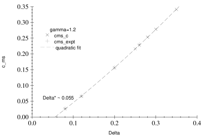
FIG. 3.: Front velocity as a function of $\Delta$, as calculated by marginal stability and measured by simulations. The marginally stable velocity is the smallest velocity for which the front is stable in its own frame against local perturbations.

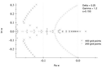
FIG. 4.: Portion of the spectrum below the marginally stable velocity. $\gamma=1.2$, $\Delta=0.25$. Two sizes of grids are shown, to give some indication of the nature of the modes in the continuum limit. Most modes not shown lie on or close to the negative real axis.

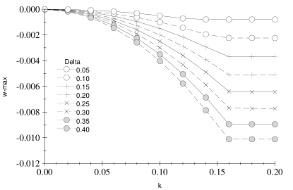
FIG. 5.: Growth rate of most unstable mode as a function of transverse wavenumber of perturbation, Witten-Sander model (9). The velocity is chosen to be $c=1.02c_{\rm ms}=1.02(2\Delta)$. Similar results are found at $c=c_{\rm ms}$, except for the offset mentioned in Figure 1.

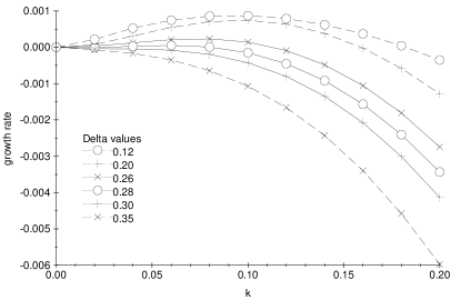
FIG. 6.: Growth rate of most unstable mode as a function of transverse wavenumber of perturbation, $\gamma$ model (11), $\gamma=1.2$ for various values of $\Delta$. Instability sets in at $\Delta^{**}\approx 0.29$.

FIG. 7.: A portion of the spectrum for $\gamma=1.2$, $\Delta=0.20$, and $k=0.10$.

- [1] D. A. Kesser, J. Koplik, and H. Levine, Adv. Phys. 37, 255 (1988).
- [2] A. Dougherty and A. Gunawardana, Phys. Rev. E 50, 1349 (1994).
- [3] Y. Sawada, A. Dougherty, and J. P. Gollub, Phys. Rev. Lett. 56, 1260 (1986).
- [4] D. G. Grier, E. Ben-Jacob, R. Clarke, and L. M. Sander, Phys. Rev. Lett. 56, 1264 (1986).
- [5] E. Ben-Jacob, H. Shmueli, O. Shochet, and A. Tenenbaum, Physica A 187, 378 (1992).
- [6] E. Ben-Jacob, O. Avidan, A. Tenenbaum, and O. Shochet, Physica A 202, 1 (1994).
- [7] H. Hentschel and A. Fine, Phys. Rev. Lett. 73, 3592 (1994).
- [8] M. C. Cross and P. C. Hohenberg, Rev. Mod. Phys. 65, 851 (1993).
- [9] O. Shochet, M.sc. thesis, Tel-Aviv University, 1992.
- [10] O. Shochet et al., Physica A 181, 136 (1992).
- [11] O. Shochet et al., Physica A 187, 87 (1992).
- [12] O. Shochet and E. Ben-Jacob, Phys. Rev. E 48, R4168 (1993).
- [13] T. Witten and L. M. Sander, Phys. Rev. Lett. 47, 1400 (1981).
- [14] E. Brener, H. Levine, and Y. Tu., Phys. Rev. Lett. 66, 1978 (1991).
- [15] Y. Tu and H. Levine, Phys. Rev. A15 45, 1044 (1992).
- [16] Y. Tu and H. Levine, Phys. Rev. A15 45, 1053 (1992).
- [17] Y. Tu, H. Levine, and D. Ridgway, Phys. Rev. Lett. 71, 3838 (1993).
- [18] J. B. Collins and H. Levine, Phys. Rev. B 31, 6119 (1985).
- [19] J. S. Langer, in Directions in Condensed Matter Physics, edited by Grinstein and Mazenko (World Scientific, 1986), pp. 164–186.
- [20] R. J. Braun, G. B. McFadden, and S. R. Coriell, Phys. Rev. E 49, 4336 (1994).
- [21] M. Uwaha and Y. Saito, Phys. Rev. A 40, 4716 (1989).
- [22] P. Keblinski, A. Maritan, F. Toigo, and J. Banavar, Phys. Rev. E 49, R4795 (1994).
- [23] F. Liu and N. Goldenfeld, Phys. Rev. A15 42, 895 (1990).
- [24] Y. Tu and H. Levine, Phys. Rev. E 48, R4207 (1994).
- [25] R. Graham and A. Schenzle, Phys. Rev. A 26, 1676 (1982).
- [26] E. Shapiro, Phys. Rev. E 48, 109 (1993).
- [27] G. Wulff, Z. Krist. 34, 449 (1901).
- [28] R. Dobrushin, R. Kotecky, and S. Shlosman, Wulff Construction: A Global Shape from Local Interaction (American Mathematical Society, Providence, Rhode Island, 1992).
- [29] D. E. Wolf, J. Phys. A 20, 1251 (1987).
- [30] J. S. Wettlaufer, M. Jackson, and M. Elbaum, J. Phys A: Math Gen. 27, 5957 (1994).
- [31] E. Ben-Jacobs et al., Physica D 14, 348 (1985).
- [32] G. Paquette, L. Chen, N. Goldenfeld, and Y. Oono, Phys. Rev. Lett. 72, 76 (1994).
- [33] W. W. Mullins and R. K. Sekerka, J. Appl. Phys. 35, 444 (1964).
- [34] B. J. Gluckman, C. B. Arnold, and J. P. Gollub, Phys. Rev. E 51, 1128 (1995).
- [35] C. C. Chow and T. Hwa, Defect-Mediated stability: an effective hydrodynamic theory of spatiotemporal chaos, on xxx.lanl.gov as cond-mat/9412041, 1994.
- [36] D. ben Avraham, M. A. Burschka, and C. R. Doering, J. Statistical Physics 60, 695 (1990).
- [37] B. P. Lee and J. Cardy, Phys. Rev. E 50, R3287 (1994).