Parity Violating Measurements of Neutron Densities

Abstract

Parity violating electron nucleus scattering is a clean and powerful tool for measuring the spatial distributions of neutrons in nuclei with unprecedented accuracy. Parity violation arises from the interference of electromagnetic and weak neutral amplitudes, and the $Z^{0}$ of the Standard Model couples primarily to neutrons at low $Q^{2}$. The data can be interpreted with as much confidence as electromagnetic scattering. After briefly reviewing the present theoretical and experimental knowledge of neutron densities, we discuss possible parity violation measurements, their theoretical interpretation, and applications. The experiments are feasible at existing facilities. We show that theoretical corrections are either small or well understood, which makes the interpretation clean. The quantitative relationship to atomic parity nonconservation observables is examined, and we show that the electron scattering asymmetries can be directly applied to atomic PNC because the observables have approximately the same dependence on nuclear shape.

I Introduction

The size of a heavy nucleus is one of its most basic properties. However, because of a neutron skin of uncertain thickness, the size does not follow from measured charge radii and is relatively poorly known. For example, the root mean square neutron radius in ²⁰⁸Pb, $R_{n}$ is thought to be about 0.25 fm larger then the proton radius $R_{p}\approx 5.45$ fm. An accurate measurement of $R_{n}$ would provide the first clean observation of the neutron skin. This is thought to be an important feature of all heavy nuclei.

The interior baryon density of a heavy nucleus is closely related to its size. The saturation density of nuclear matter $\rho_{0}$ is a fundamental concept central to nuclear structure, the nature of the interactions between nucleons, models of heavy ion collisions and applications of dense matter in Astrophysics. The value of $\rho_{0}$ is inferred from the central density of heavy nuclei, most notably ²⁰⁸Pb. One then corrects for the effects of surface tension and Coulomb interactions (which tend to cancel) and deduces the saturation density of an infinite system.

However, present estimates of $\rho_{0}$ are based only on the known proton density. Thus $\rho_{0}$ is uncertain because we do not have accurate information on the central neutron density. An accurate measurement of the neutron radius $R_{n}$ will constrain the average interior neutron density and help refine our knowledge of $\rho_{0}$.

Ground state charge densities have been determined from elastic electron scattering, see for example ref.[1]. Because the densities are both accurate and model independent they have had a great and lasting impact on nuclear physics. They are, quite literally, our modern picture of the nucleus.

In this paper we discuss future parity violating measurements of neutron densities. These purely electro-weak experiments follow in the same tradition and can be both accurate and model independent. Neutron density measurements may have implications for nuclear structure, atomic parity nonconservation (PNC) experiments, isovector interactions, the structure of neutron rich radioactive beams, and neutron rich matter in astrophysics. It is remarkable that a single measurement has so many applications in atomic, nuclear and astrophysics.

Donnelly, Dubach and Sick[2] suggested that parity violating electron scattering can measure neutron densities. This is because the $Z-$boson couples primarily to the neutron at low $Q^{2}$. Therefore one can deduce the weak-charge density and the closely related neutron density from measurements of the parity-violating asymmetry in polarized elastic scattering. This is similar to how the charge and proton densities are deduced from unpolarized cross sections.

Of course the parity violating asymmetry is very small, of order a part per million. Therefore measurements were very difficult. However, a great deal of experimental progress has been made since the Donnelly et. al. suggestion, and since the early SLAC experiment[3]. This includes the Bates ¹²C experiment[4], Mainz ⁹Be experiment[5], SAMPLE[6] and HAPPEX[7]. The relative speed of the HAPPEX result and the very good helicity correlated beam properties of CEBAF show that very accurate parity violation measurements are possible. Parity violation is now an established and powerful tool.

For example, the HAPPEX result suggests that strange quarks do not make large contributions to the nucleon’s electric form factor. Clearly additional experiments should (and will) be done to further measure strange quarks. However, it is important to also apply parity violation to other physics objectives such as neutron densities. This will allow one to take maximum advantage of parity violation.

It is important to test the Standard Model at low energies with atomic PNC, see for example the Colorado measurement in Cs[8, 9]. These experiments can be sensitive to new parity violating interactions such as additional heavy $Z-$bosons. Furthermore, by comparing atomic PNC to higher $Q^{2}$ measurements, for example at the $Z$ pole, one can study the momentum dependence of Standard model radiative corrections. However, as the accuracy of atomic PNC experiments improves they will require increasingly precise information on neutron densities[10, 11]. This is because the parity violating interaction is proportional to the overlap between electrons and neutrons. In the future the most precise low energy Standard Model test may involve the combination of an atomic PNC measurement and parity violating electron scattering to constrain the neutron density.

Unfortunately, atomic PNC suffers from atomic theory uncertainties in the electron density at the nucleus. This motivates future atomic experiments involving isotope ratios where the atomic theory cancels. However, these ratios may require even more nuclear structure information on isotope differences of neutron densities. Parity violating electron scattering measurements of isotope differences is beyond the scope of this paper. Instead we focus on simpler measurements of the neutron density in a single closed (sub)shell isotope. These measurements should provide an important first step for later work on isotope differences.

There have been many measurements of neutron densities with strongly interacting probes such as pion or proton elastic scattering, see for example ref. [12]. We discuss some of these in section II. Unfortunately, all such measurements suffer from potentially serious theoretical systematic errors. As a result no hadronic measurement of neutron densities has been generally accepted by the field. Because of the uncertain systematic errors, modern mean field interactions are typically fit without using any neutron density information, see for example refs.[13, 14].

An electro-weak measurement of the neutron density in a nucleus such as ²⁰⁸Pb may allow the calibration of strongly interacting probes. By requiring that the hadronic reaction theory reproduce the electro-weak measurement one should reduce theoretical errors. This is analogous to using beta decay to calibrate $(p,n)$ probes of Gamow Teller strength. Once proton nucleus elastic scattering is calibrated it should be possible to study neutron densities in a variety of other nuclei including radioactive beams.

Finally, there is an interesting complementarity between neutron radius measurements in a finite nucleus and measurements of the neutron radius of a neutron star. Both provide information on the equation of state of dense matter. In a nucleus, $R_{n}$ is sensitive to the surface symmetry energy or the symmetry energy at low densities while the neutron star radius depends on the symmetry energy at high densities.

In the future we expect a number of improving radius measurements for nearby isolated neutron stars. For example, from the measured luminosity and surface temperature one can deduce an effective surface area and radius from thermodynamics. Candidate stars include Geminga[15] and RX J185635-3754[16].

This paper is organized as follows. In section II we discuss the present theoretical and experimental knowledge of neutron densities. In section III we present general considerations for neutron density measurements and include some experimental issues in section IV. Section V discusses many possible theoretical corrections and shows that the interpretation of a measurement is very clean. The relationship between neutron density measurements and atomic parity nonconservation experiments is discussed in section VI. Finally we conclude in section VII.

II Present Knowledge of Neutron Densities

In this section we discuss our present knowledge of neutron densities. Unfortunately, neutron density uncertainties have not been extensively discussed in the literature. Fortson et al.[17] give some discussion on the present uncertainties in neutron densities and how this uncertainty impacts atomic PNC. They claim a relatively large error in the neutron radius $R_{n}$ of order 10%.

We believe the most accurate information comes from theory. As we discuss below, mean field models predict a relatively small spread in neutron densities once the effective interaction is constrained to reproduce observed charge densities and binding energies. We also discuss neutron density measurements with elastic magnetic electron scattering and strongly interacting probes.

A Neutron Density Theory

Mean field models have been very successful at reproducing many features of nuclear charge densities including measured charge radii. Figure  1, adapted from Ring et al.[14], shows differences between neutron $R_{n}$ and proton radii $R_{p}$ for a range of nuclei for calculations based on two typical interactions. A nonrelativistic zero range Skyrme force gives $R_{n}-R_{p}\approx 0.1$Fm for ²⁰⁸Pb while a relativistic mean field calculation gives $R_{n}-R_{p}\approx 0.3$Fm. We don’t claim that these two calculations represent extreme values. Rather they represent the range in $R_{n}-R_{p}$ for two typical classes of interactions.

In order for the theoretical error to be less then the spread in Figure  1 one must demonstrate that one (or both) of the calculations is unrealistic. While this may be possible in the future, it has not yet been demonstrated since both calculations are in common use. Of course, the real uncertainty could be larger then the spread in Figure  1 if the two calculations do not probe the full parameter space of possible mean field interactions. In the absence of more precise uncertainties, one can take this spread $\approx 0.2$Fm as some measure of the present uncertainty in $R_{n}$. This compares to a charge radius of 5.51 Fm. A one percent measurement of $R_{n}$ with an accuracy of about $0.05$Fm can clearly distinguish between the two forces. Furthermore, it can distinguish either prediction for $R_{n}-R_{p}$ from zero thus cleanly observing the neutron skin.

We note that the relativistic mean field calculation with its larger $R_{n}$ predicts a significantly smaller central neutron density then does the Skyrme interaction. What gives rise to the differences between the two calculations? Unfortunately, there is not much discussion in the literature. We speculate that some of the difference arises because the relativistic mean field calculation uses a finite range force while the Skyrme interaction is zero range. There is an attractive interaction between the neutrons and the protons. A finite range force allows the neutrons to sit at a slightly larger radius and still feel much of the attraction. Therefore we expect finite range interactions to predict slightly larger $R_{n}-R_{p}$ then for zero range forces.

Once mean field interactions are constrained to reproduce a neutron radius measurement in a stable nucleus such as ²⁰⁸Pb they can make improved predictions for a variety of unstable nuclei. We note that the nonrelativistic Skyrme force SKX[18] is designed for use in both normal and exotic nuclei such as ⁴⁸Ni, ⁶⁸Ni and ¹⁰⁰Sn. One example of relativistic mean field calculations for neutron rich nuclei is ref.[19]. The structure of exotic nuclei is important for Astrophysics and for radioactive beams.

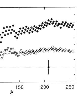
FIG. 1.: The difference between neutron radii $R_{n}=r_{n}$ and proton radii $R_{p}=r_{p}$ for several nuclei of different mass number $A$. The filled symbols are for the relativistic mean field NL1 interaction while the open symbols are for the nonrelativistic zero range Skyrme skiii interaction. This figure is taken from calculations of Ring et.al [14]. A possible 1% measurement in ²⁰⁸Pb is indicated by the error bar which has been arbitrarily placed at $R_{n}-R_{p}=0$.

B Neutron Density Measurements

There have been many measurements sensitive to neutron densities. Originally neutron radii were extracted from Coulomb energy differences[20]. However, it is now thought these measurements are sensitive to isospin violating interactions. Next $(p,d)$ and $(d,t)$ stripping reactions are sensitive to the tail in the neutron density at very large radius[21]. However, stripping reactions are not directly sensitive to the interior density. Because the interior density is much larger then that in the tail it contributes significantly to $R_{n}$. Therefore $R_{n}$ can not be extracted from stripping experiments without making model assumptions.

Proton nucleus elastic scattering is sensitive to both the surface and interior neutron density[12]. Typically this data is analyzed in an impulse approximation where a nucleon-nucleon interaction is folded with the nucleon density. Unfortunately, there are corrections to the impulse approximation from for example multiple scattering and medium modifications to the NN interaction whose uncertainties are difficult to quantify. Limitations in the theoretical analysis can show up as an unphysical dependence of the extracted neutron density on the beam energy.

Future work on extracting neutron densities from proton scattering would be very useful. This could take advantage of advances in full folding calculations. Furthermore, neutron-nucleus elastic scattering data would be very helpful. Comparing proton- and neutron-nucleus scattering could help constrain the effective proton-neutron interaction. Finally, if proton-nucleus scattering can be calibrated to accurately reproduce a neutron density measurement in a stable nucleus then it could be applied to a wide variety of other nuclei. For example, it is possible to measure proton-nucleus scattering from radioactive beams with a hydrogen target in inverse kinematics.

Finally, data comparing the elastic scattering of positive and negative pions from nuclei exist[22], but again there are uncertainties in the analysis[10]. These methods are not really directly sensitive to the neutron density.

Elastic magnetic electron scattering is an established tool for nuclear structure. Furthermore, magnetic scattering is directly sensitive to the neutron magnetic moment. Thus information about valence neutron radii can be extracted. Note, more calculations of the effects of Coulomb distortions on magnetic scattering from heavy nuclei would be useful. See for example [23]. However most of the neutrons in a heavy nucleus are coupled to spin zero and make no contribution to the magnetization. Therefore, magnetic scattering can not directly determine $R_{n}$.

We conclude that no existing measurement of neutron densities or radii has an established accuracy of one percent. While some conflicting claims may have been made, all hadronic probes of $R_{n}$ suffer from some reaction mechanism uncertainties. As a result there is no agreement in the community that any measurement has the requisite accuracy. Even if it is possible to reach one percent accuracy with a hadronic probe, this accuracy has not yet been established.

III General Considerations

In this section we illustrate how parity violating electron scattering measures the neutron density. For simplicity, this section uses the plane-wave Born approximation and neglects nucleon form factors. The effects of Coulomb distortions and form factors are included in section V. These are necessary for a quantitative analysis but they do not invalidate the simple qualitative picture presented here.

The electron interacts with a nucleus by exchanging either a photon or a $Z_{0}$ boson. The propagator involved in the interaction is of the form

$$\frac{1}{Q^{2}+M_{B}^{2}}$$ (1)

where $M_{B}$ is the mass of the exchanged boson. For the photon $M_{B}=0$, whereas for the $Z_{0}$ the mass term dominates. Since for elastic scattering from nuclei, $M_{Z}^{2}\gg Q^{2}$, the photon term is much larger than the $Z_{0}$ term. Note, we use the convention $Q^{2}=-{q_{\mu}}^{2}>0$.

Another difference between the exchange of the photon and the $Z_{0}$ is the couplings to both the electron and the nucleons. The photon has purely vector couplings, and couples only to protons at $Q^{2}=0$. We note that for the spinless nuclei considered here, the magnetic moments cannot contribute. The $Z_{0}$ has both vector and axial vector couplings. Since the nuclei being considered are spinless, the net axial coupling to the nucleus is absent. In contrast to the case for photons, the $Z_{0}$ has a much larger coupling to the neutron than the proton. In addition, the $Z_{0}$ has a large axial coupling to the electron that results in a parity-violating amplitude. The effect of the parity-violating part of the weak interaction may be isolated by measuring the parity-violating asymmetry

$$A_{LR}=\frac{\sigma_{R}-\sigma_{L}}{\sigma_{R}+\sigma_{L}},$$ (2)

where $\sigma_{L(R)}$ is the cross section for the scattering of left(right) handed electrons. In contrast to the cross section, the asymmetry is sensitive to the distribution of the neutrons in the nucleus. The $Z_{0}$ also has a vector coupling to the electron, but this term is neglected because the contribution cannot be isolated from the dominant photon amplitude.

The implication of the above is that the potential between an electron and a nucleus to a good approximation may be written

$$\hat{V}(r)=V(r)+\gamma_{5}A(r)$$ (3)

where the usual electromagnetic vector potential is

$$V(r)=\int d^{3}r\prime Z\rho(r\prime)/|\vec{r}-\vec{r}\,\prime|$$ (4)

and where the charge density $\rho(r)$ is closely related to the point proton density $\rho_{p}(r)$ given by

$$Z\rho_{p}(r)=\sum_{p}\langle\psi_{p}^{\dagger}(r)\psi_{p}(r)\rangle.$$ (5)

The axial potential $A(r)$ depends also on the neutron density:

$$N\rho_{n}(r)=\sum_{p}\langle\psi_{n}^{\dagger}(r)\psi_{n}(r)\rangle.$$ (6)

It is given by

$$A(r)={G_{F}\over 2^{3/2}}[(1-4{\rm sin}^{2}\theta_{W})Z\rho_{p}(r)-N\rho_{n}(r)]$$ (7)

The axial potential has two important features:

1. It is much smaller than the vector potential, so it is best observed by measuring parity violation. It is of order one eV while $V(r)$ is of order MeV.

2. Since $\sin^{2}\theta_{W}\sim 0.23,\ (1-4\sin^{2}\theta_{W})$ is small and $A(r)$ depends mainly on the neutron distribution $\rho_{n}(r)$.

The electromagnetic cross section for scattering electrons with momentum transfer $q=(Q^{2})^{1/2}$ is given by

$$\frac{d\sigma}{d\Omega}=\frac{d\sigma}{d\Omega}_{\rm Mott}|F_{p}(Q^{2})|^{2}$$ (8)

where

$$F_{p}(Q^{2})=\frac{1}{4\pi}\int d^{3}rj_{0}(qr)\rho_{p}(r)$$ (9)

is the form factor for protons, where $j_{0}$ is the zero’th spherical Bessel function. From $F_{p}(Q^{2})$, one may determine $R_{p}$. One can also define a form factor for neutrons

$$F_{n}(Q^{2})=\frac{1}{4\pi}\int d^{3}rj_{0}(qr)\rho_{n}(r)$$ (10)

Thus $R_{n}$ may be determined if $F_{n}(Q^{2})$ is known.

In Born approximation the parity-violating asymmetry involves the interference between $V(r)$ and $A(r)$. It is,

$$A_{LR}=\frac{G_{F}Q^{2}}{4\pi\alpha\sqrt{2}}\Biggl{[}4\sin^{2}\theta_{W}-1+\frac{F_{n}(Q^{2})}{F_{p}(Q^{2})}\Biggr{]}$$ (11)

The asymmetry is proportional to $Q^{2}/M_{Z}^{2}$ (since $G_{F}\propto M_{Z}^{-2}$) which is just the ratio of the propagators of Eq. 1. Since 1-4sin${}^{2}\theta_{W}$ is small and $F_{p}(Q^{2})$ is known we see that $A_{LR}$ directly measures $F_{n}(Q^{2})$. Therefore, $A_{LR}$ provides a practical method to cleanly measure the neutron form factor and hence $R_{n}$.

IV Experimental Issues

The experimental techniques for measuring small asymmetries of order 1 ppm have been successfully deployed in parity experiments at electron scattering facilities [3]-[7]. The following general considerations applies to these experiments.    1)  Often a compromise must be chosen between optimizing the parity violating signal and the signal to noise ratio. The asymmetry generally increases with $Q^{2}$ while the cross section decreases, which leads to an optimum choice of kinematics.    2)  A major challenge for these measurements is to maintain systematic errors associated with helicity reversal at the $\approx 10^{-8}$ level. There must be at least one, and preferably several, methods to reverse the helicity. Many reversals are needed during an experiment, and they should follow a rapid and random sequence to avoid any correlation with noise. The helicity reversals should be uncoupled to other parameters which affect the cross section. Experiments must measure the sensitivity of the cross section to these parameters, as well as the helicity correlated differences in them.    3)  Electronic pickup of the helicity correlated signals can cause a false asymmetry, as can helicity correlated deadtime.    4)  In a count rate limited experiment in which the detected particles must be integrated in order to get the desired accuracy in a reasonable time, the linearity of the detection system and the susceptibility to backgrounds are important issues. For the high-rate experiments considered here, the radiation hardness of the detectors is also an issue.    5)  The beam polarization must be measured with high precision. Online monitoring is possible using a Compton polarimeter which is cross-calibrated using Møller and Mott polarimeters whose absolute calibrations may be $\approx$1%.

A Choices of Target and Kinematics

There are two nuclei which are of interest for a measurement of the neutron radius to 1% accuracy, ²⁰⁸Pb and ¹³⁸Ba. They are equally accessible experimentally. Pb has the advantage that it has the largest known splitting to the first excited state (2.6 MeV) of any heavy nucleus, and thus lends itself well to the use of a flux integration technique. Also Pb has been very well studied, and with its simple structure is a good first test case for nuclear theory. Ba has the advantage that it is one of the nuclei being used for an atomic physics test of the Standard Model.

The choice of kinematics for a first measurement is guided by the objective of minimizing the running time required for a 1% accuracy in $R_{n}$. Figure  2 shows for the case of ²⁰⁸Pb the three ingredients which enter into this optimization:  the cross section $d\sigma/d\Omega$, the parity violating asymmetry $A$, and the sensitivity to the neutron radius $\epsilon=dA/A=(A1-A)/A$ where $A$ is the asymmetry computed from a mean field theory (MFT) calculation[24] and $A1$ is the asymmetry for the MFT calculation in which the neutron radius is increased by 1%. These three ingredients, which each vary with energy and angle, are plotted in figure  2 for a beam energy of 0.85 GeV. As we will show below, 0.85 GeV turns out to be the energy which minimizes the running time for a 1% $R_{n}$ determination. Using magnetic spectrometers with high resolution to isolate elastically scattered electrons, the optimal kinematics can be determined from the allowable settings for angle and momentum of the spectrometer by searching for the the minimum running time, which is equivalent to maximizing the product

$${\rm FOM}\hskip 3.61371pt\times\hskip 3.61371pt{\epsilon}^{2}\hskip 3.61371pt=\hskip 3.61371ptR\times A^{2}\times{\epsilon}^{2}$$ (12)

where R is the detected rate and is proportional to $d\sigma/d\Omega$, and “FOM” is the conventionally defined figure of merit for parity experiments, FOM  $=R\times A^{2}$. Note that rather than only maximizing the conventional FOM, parity violating neutron density measurements take into account the sensitivity ($\epsilon$) to $R_{n}$ which varies with kinematics.

As an example, we have performed the optimization for the Jefferson Lab Hall A high resolution spectrometers supplemented by septum magnets that allow to reach $6^{\circ}$ scattering angle. The calculations take into account the averaging over the finite acceptance and the energy resolution needed to discriminate inelastic levels. Figure  2 shows the product ${\rm FOM}\hskip 3.61371pt\times\hskip 3.61371pt{\epsilon}^{2}$ for ²⁰⁸Pb which peaks at E = 0.85 GeV. Similar calculations for ¹³⁸Ba shows an optimum at 1.0 GeV (figure  3). For both these nuclei the running time $T$ in days to reach a 1% accuracy in $R_{n}$ is approximately $T\approx 7/(P^{2}I\Omega)$ days, where $P$ is the polarization ($P\approx 0.8$ is achievable), $I$ is the average beam current in $\mu$A ($I\approx 50\mu$A is achievable) and $\Omega$ is the solid angle acceptance of the spectrometer in steradians. This optimum point corresponds to $q=0.45\hskip 3.61371pt{\rm fm}^{-1}$ and 0.53 $\hskip 3.61371pt{\rm fm}^{-1}$ for Pb and Ba respectively. In the plots of ${\rm FOM}\times{\epsilon}^{2}$ one can see a secondary ridge where one might want to perform a second measurement at higher $Q^{2}$ to check the shape dependence. Here the experimental running time becomes longer but the required accuracy in $R_{n}$ can be reduced. As an example, for ²⁰⁸Pb at E = 1.3 GeV,  $\theta=8^{\circ}$, corresponding to $q=0.92\hskip 3.61371pt{\rm fm}^{-1}$ the running time to reach 2% in $R_{n}$ is $T\approx 19/(P^{2}I\Omega)$ days.

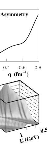
FIG. 2.: Cross section, parity violating asymmetry, and sensitivity to $R_{n}$ for ²⁰⁸Pb elastic scattering at 0.85 GeV. The fourth plot shows the variation of FOM$\times{\epsilon}^{2}$ with energy and angle, showing an optimum at 0.85 GeV for a $6^{\circ}$ scattering angle which corresponds to $q\hskip 2.168pt=\hskip 2.168pt0.45\hskip 2.168pt{\rm fm}^{-1}$.

To reduce the running time, a thick target is needed;  the main issues are:    1)  For a given energy resolution required to discriminate excited states, there is an optimum target thickness ($\approx$ 10% radiation length) that maximizes the rate in the detector. As the target becomes thicker the radiative losses decrease the rate.    2)  If at the low-$Q^{2}$ where the experiments run the rates from some low level inelastic states are sufficiently small and understood theoretically, one may tolerate accepting them into the detector, thus allowing to integrate more of the radiative tail, typically up to 4 MeV.    3)  To improve the heat load capability of the target, one may use various “cooling agents”, such as laminations of diamond interleaved with the target material. One must have sufficient knowledge of the effect on the parity signal. For example, if one accepts 2% rate from ¹²C and the theory is understood to 1%, the systematic error is only 0.02%. The theoretical error is discussed in section V.

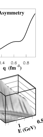
FIG. 3.: Same as figure  2 except for ¹³⁸Ba at 1.0 GeV

V Corrections to the Asymmetry

In this section we document a number of corrections to the parity violating asymmetry and show that they have small uncertainties. Therefore the interpretation of a measurement should be clean. We consider coulomb distortions, strangeness and the neutron electric form factor, parity admixtures, dispersion corrections, meson exchange currents, shape dependence, isospin admixtures, role of excited states and the effect of target impurities.

A Coulomb distortions

By far the largest known correction to the asymmetry comes from coulomb distortions. By coulomb distortions we mean repeated electromagnetic interactions with the nucleus remaining in its ground state. All of the $Z$ protons in a nucleus can contribute coherently so distortion corrections are expected to be of order $Z\alpha/\pi$. This is 20 % for ²⁰⁸Pb.

Distortion corrections have been accurately calculated in ref.[24]. Here the Dirac equation was numerically solved for an electron moving in a coulomb and axial-vector weak potentials. From the phase shifts, all of the elastic scattering observables including the asymmetry can be calculated.

There are many checks on the numerics of this calculation. First, known cross sections including those at large angles are reproduced. Second, the code reproduces known plane wave asymmetries. Finally, the sensitivity to the subtraction between helicities is checked by varying the strength of the weak potential. We note that the forward angle asymmetry is much easier to calculate then the backward angle cross section because the cross section involves extreme cancellations in the sum over partial waves. It is expected that the numerical accuracy in the asymmetry is significantly better then 1%. However, the code neglects terms involving the electron mass over the beam energy. These are of order 0.1%. There are now a number of independent codes which calculate the effects of coulomb distortions[19, 25, 26] and verify the accuracy of ref.[24].

In summary, distortion corrections are larger then the experimental error. Furthermore, they modify the sensitivity to the neutron radius. However, they have been calculated with an accuracy significantly better then the expected 3% experimental error.

Finally, since the charge density is known it should be possible to “invert” the coulomb distortions and deduce from the measured asymmetry the value of a Born approximation equivalent weak form factor at the momentum transfer $Q^{2}$ of the experiment. Thus, the main result of the measurement is the weak form factor $F_{W}(Q^{2})$ which is the Fourier transform of the weak charge density $\rho_{W}(r)$,

$$F_{W}(Q^{2})=\int d^{3}rj_{0}(qr)\rho_{W}(r).$$ (13)

This can be directly compared to mean field or other theoretical calculations. Note, $F_{W}$ will not be determined by comparing plane wave calculations to data. Instead, for example, a range of model weak densities could be adjusted until full distorted wave calculations reproduce the experimental asymmetry. Then, Eq. 13 is used to calculate $F_{W}(Q^{2})$. In principle this procedure is slightly model dependent because full distorted wave calculations need some information on $F_{W}(Q^{2})$ for $q$ different from the single measurement. However this model dependence is expected to be very small and can be explored by studying a variety of model densities.

B Strangeness and neutron electric form factors

From $F_{W}$ the root mean square radius of the weak charge distribution $R_{W}$ can be determined, see section VF. The weak radius, in turn, can be related to the radius of the neutron distribution after making appropriate corrections. We emphasize that the experiment measures a well defined form factor of the weak charge distribution and that this can be directly compared to mean field models without any additional corrections. However, if one wishes to go further and extract a point neutron radius one must correct for possible strange quark contributions and other nucleon form factors. We discuss these here. In addition, there could be meson exchange currents which we discuss in a later subsection.

The electric form factors for the coupling of a $Z^{0}$ to the proton $G_{p}^{Z}$ and neutron $G_{n}^{Z}$ are,

$$G_{p}^{Z}={1\over 4}(G_{p}-G_{n})-{\rm sin}^{2}\Theta G_{p}-{1\over 4}G_{s},$$ (14)

$$G_{n}^{Z}={1\over 4}(G_{n}-G_{p})-{\rm sin}^{2}\Theta G_{n}-{1\over 4}G_{s}.$$ (15)

We are only interested in electric form factors since magnetic form factors make no contribution for a spin zero target. Therefore we omit the label $E$ for clarity. The proton (neutron) electromagnetic form factor is $G_{p}$ ($G_{n}$). The strange quark form factor is $G_{s}$ and this is assumed the same for neutrons and protons.

We fold these form factors with point proton $\rho_{p}$ and neutron $\rho_{n}$ densities to obtain the weak charge density $\rho_{W}$,

$$\rho_{W}(r)=4\int d^{3}r^{\prime}\bigl{[}G_{n}^{Z}(r^{\prime})N\rho_{n}(|{\bf r-r^{\prime}}|)+G_{p}^{Z}(r^{\prime})Z\rho_{p}(|{\bf r-r^{\prime}}|)\bigr{]}.$$ (16)

The densities are normalized,

$$\int d^{3}r\rho_{p}(r)=1,$$ (17)

$$\int d^{3}r\rho_{n}(r)=1,$$ (18)

and

$$\int d^{3}r\rho_{W}(r)=Q_{W},$$ (19)

where the weak charge of the nucleus is,

$$Q_{W}=-N+(1-4{\rm sin}^{2}\Theta)Z.$$ (20)

The proton $R_{p}$, neutron $R_{n}$ and weak $R_{W}$ radii are defined,

$$R^{2}_{p}=\int d^{3}rr^{2}\rho_{p}(r),$$ (21)

$$R_{n}^{2}=\int d^{3}rr^{2}\rho_{n}(r),$$ (22)

and

$$R_{W}^{2}={1\over Q_{W}}\int d^{3}rr^{2}\rho_{W}(r).$$ (23)

It is a simple matter to calculate the weak radius from Eq. 16,

$$-Q_{W}R_{W}^{2}\hskip 7.22743pt=\hskip 7.22743ptNR_{n}^{2}+(4{\rm sin}^{2}\Theta-1)ZR_{p}^{2}+\bigl{[}N+(4{\rm sin}^{2}\Theta-1)Z\bigr{]}r_{p}^{2}\hskip 86.72377pt$$

$$\hskip 72.26999pt+\hskip 7.22743pt\bigl{[}Z+(4{\rm sin}^{2}\Theta-1)N\bigr{]}r_{n}^{2}\hskip 7.22743pt+\hskip 7.22743pt(N+Z)r_{s}^{2}.$$ (24)

Here $r_{p}^{2}$ is the mean square charge radius of the proton, $r_{n}^{2}$ the square of the neutron charge radius and $r_{s}^{2}$ is the mean square strangeness radius.

Assuming the neutron radius is much larger then $R_{n}-R_{p}$ and $r_{p}$ the above reduces to

$$R_{W}\approx R_{n}+{Z(1-4{\rm sin}^{2}\Theta)\over N+(4{\rm sin}^{2}\Theta-1)Z}(R_{n}-R_{p}){\hskip 144.54pt}$$

$${\hskip 86.72377pt}+{1\over 2R_{n}}\bigl{\{}r_{p}^{2}+{Z+(4{\rm sin}^{2}\Theta-1)N\over N+(4{\rm sin}^{2}\Theta-1)Z}r_{n}^{2}+{N+Z\over N+(4{\rm sin}^{2}\Theta-1)Z}r_{s}^{2}\bigr{\}}.$$ (25)

For ²⁰⁸Pb, assuming $R_{n}\approx 5.50$ fm and sin${}^{2}\Theta=0.23$, we have

$$R_{W}\approx R_{n}+0.055(R_{n}-R_{p})+0.061(\pm 0.002)-0.0089(\pm 0.0003)-0.011\rho_{s}$$ (26)

in fm. The 0.061 is from the charge radius of the proton and the -0.0089 from the charge radius of the neutron[27].

The last term in Eq. 26 is from strange quark contributions. The strange quark form factor $G_{s}$ has been parameterized with $\rho_{s}$,

$$G_{s}(Q^{2})=\rho_{s}\tau/(1+4.97\tau)^{2},$$ (27)

and $\tau=Q^{2}/4M^{2}$. We aim to measure $R_{W}$ to 1% or about 0.055 fm. Therefore, strange quarks will contribute less then 1% as long as,

$$|\rho_{s}|<5.$$ (28)

This is a very mild requirement which is already strongly supported by existing experiments. For example, the HAPPEX measurement [7],

$$G_{E}^{s}+0.39G_{M}^{s}(Q^{2}=0.48{\rm GeV}^{2})=0.023\pm 0.043,$$ (29)

and the SAMPLE measurement [6],

$$G_{M}^{s}(Q^{2}=0.1{\rm GeV}^{2})=0.23\pm 0.44,$$ (30)

yield,

$$0.011\rho_{s}=-0.0043\pm 0.021{\rm fm}.$$ (31)

The errors quoted are combined statistical and systematic and we have assumed the form of Eq. 27 for the $Q^{2}$ dependence of the strange form factor. Equation 31 limits the strangeness contributions to $R_{n}$ to 0.4%. Note, if one assumes a different $Q^{2}$ dependence than Eq. 27, it may be possible to somewhat weaken this limit. However, additional measurements in the near future will significantly tighten the constraints on strange quarks and clearly rule out $|\rho_{s}|>5$.

Likewise, the neutron electric form factor contributes far less then 1% to $R_{W}$. Theoretical models have $R_{n}-R_{p}\leq 0.3$ fm, so the second term in Eq. 25 is also less then 1%. Indeed to 1%, the neutron radius directly follows from the measured weak radius,

$$R_{n}\approx R_{W}-0.06{\rm fm}$$ (32)

We conclude that the contribution of strange quarks or the neutron electric form factor are not issues for a neutron radius measurement. The radius of the neutron density of a heavy nucleus can be accurately determined from the measured weak radius.

C Parity Admixtures

The spin zero ground state of ²⁰⁸Pb need not be a parity eigenstate. There is probably some small admixture of $0^{-}$. However, so long as the initial and final states are spin zero, this parity admixture can not produce a parity violating asymmetry in Born approximation[28]. A multipole decomposition of the virtual photon has a $0^{+}$ coulomb but no $0^{-}$ multipole. So long as the exchanged virtual photon is spin zero, there is no parity violating interference because there is only a single operator. This statement is true regardless of the parity of the initial or final states or if the photon coupling involves a parity violating meson exchange current. Therefore, parity admixtures should not be an issue for elastic scattering from a spin zero nucleus.

D Meson Exchange Currents

Meson exchange currents MEC can involve parity violating meson couplings. These are not expected to be important for a spin zero target, see the subsection on parity admixtures above. Meson exchange currents could also change the distribution of weak charge in a nucleus. However, mesons are only expected to carry weak charge over a distance much smaller then $R_{n}$. This should not lead to a significant change in the extracted neutron radius. Let $r_{MEC}^{2}$ be the square of the average distance weak charge is moved by MEC. Then following Eq. 25 the correction to the weak radius will be of order $r_{MEC}^{2}/R_{n}$. This is expected to be very small because $R_{n}$ is large.

This same result can be viewed another way. Figure  4 shows a schematic diagram of the weak charge density. In the interior region the density is more or less constant. In this region, MEC have very little effect. The density is simply the conserved weak charge divided by the volume. It does not matter if the weak charge resides on the nucleons or on mesons going between the nucleons. The only effect of MEC is to slightly change the surface thickness. This is indicated by the dotted line in Fig.  4. This change in surface thickness will only lead to a very small change in the weak radius. We conclude that MEC are unlikely to be an issue for the interpretation of the weak radius.

E Dispersion corrections

By dispersion corrections we mean multiple electromagnetic or weak interactions where the nucleus is excited from the ground state in at least one intermediate state. At the low momentum transfers considered here, the elastic cross section involves a coherent sum over the $Z$ protons and is of order $Z^{2}$. In contrast, the incoherent sum of all inelastic transitions is only of order $Z$. Therefore we expect dispersion corrections to be of order $\alpha/Z$. This is negligible.

F Shape dependence and Surface Thickness

In principle, the weak radius follows from the derivative of a form factor evaluated at zero $Q^{2}$. In practice, the measurement will be carried out at a small but nonzero $Q^{2}$. Thus the extraction of the weak radius from the measured form factor may depend slightly on the assumed surface thickness.

We emphasize, one primary use of a measurement is to calibrate mean field models of neutron densities. One can simply calculate the weak form factor, Eq. 13, and directly compare theory and experiment without any model dependence or the need to extract a neutron radius. However, if one wishes to extract a neutron radius one must address the dependence of the radius on the shape of the neutron distribution. One is most sensitive to the surface thickness.

For example, if the weak density of ²⁰⁸Pb is modeled as a Wood Saxon with radius parameter $c$,

$$\rho_{W}(r)=\rho_{0}/\bigl{\{}{\rm exp}[(r-c)/z]+1\bigr{\}},$$ (33)

then the surface thickness parameter $z\approx 0.55$ fm must be known to $\pm 0.14$ fm in order to extract $R_{W}$ to 1% from an asymmetry measurement at the proposed $Q^{2}=0.008$ GeV². Thus the surface thickness or $z$ must be known to only 25 % in order to extract $R_{n}$.

We believe the surface thickness of the weak density is known to much better then 25% for at least two reasons. First, the surface thickness is strongly constrained by the known surface and single nucleon separation energies. At large $r$ the weak density is dominated by the most weakly bound neutron. This decays exponentially with a known separation energy. Therefore the large $r$ behavior of the weak density is known. At somewhat smaller radii the density is controlled by the surface energy. The very abrupt change in density, necessary for a small surface thickness, implies a very high surface energy. Any model with a very small surface thickness will fail to reproduce the known binding energies of a range of nuclei. As a result, all mean field models, that we are aware of, have only a small spread in surface thickness –much less then 25%– if they reproduce binding energies .

Second, the surface thickness of the weak density is constrained by the measured surface thickness of the charge density. Perhaps the easiest way to change the surface thickness of the neutron density is to change the thickness of both the protons and neutrons. However, this will quickly conflict with the measured charge density. Therefore, one has to try and change the surface thickness of the neutrons without changing the proton density. This will necessitate large separations in both energy and position between protons and neutrons. To accomplish this, one will need energetic isovector interactions which in turn will change the binding energies of nuclei as a function of N or Z and ruin agreement with known masses.

Note, present mean field models do an excellent job reproducing the surface thickness of measured charge densities. This is a nontrivial check. Although one or more parameters of mean field forces are often fit to charge radii, the detailed form of the surface density is not fit. Therefore the excellent agreement between theory and experiment in the surface region demonstrates both the power and basic correctness of these arguments that the surface thickness is strongly constrained by measured binding energies.

We illustrate the above points in Fig.  5 This shows the charge density in ²⁰⁸Pb. A figure for the weak density would be similar. Conventional mean field models, thin dashed and dotted curves, agree very well with the measured surface thickness (region beyond r=5 fm). (We note that a low $Q^{2}$ measurement is insensitive to the interior density.) In contrast the thick dashed curve shows a relativistic mean field model with a very incorrect surface energy[29]. This calculation has an incompressibility (which is closely related to the surface energy) more then a factor of two too large. This error is well outside of present uncertainties. Therefore the surface properties of this calculation can be ruled out. Nevertheless even with this large error, the surface thickness disagrees with data and other calculations by only 10%. Since this is less then 25% there would be no problem using this incorrect surface to extract the neutron radius to 1%.

We state the results of this section in a slightly different language. This measurement is sensitive to the surface thickness at only the 25% level, while it is sensitive to the radius at the 1% level. Since 25% is much larger then the present spread in surface thickness of mean field models one will not learn new information about the surface. Instead a 1% constraint on the radius does provide important new information on the radius because present models have a larger spread then 1%.

Finally, uncertainties from the surface thickness are even less important in extracting weak charge information for atomic parity experiments. This is because the atomic experiments depend on the surface thickness in somewhat similar ways to the electron scattering asymmetry. As a result, some of the error from the unknown surface thickness cancels in comparing the two experiments. Therefore, one could tolerate an uncertainty in the surface thickness of more then 25% and still interpret the atomic experiment. This is discussed in section VI.

We don’t believe the dependence on the surface thickness is a problem. Nevertheless, if one wanted to reduce the sensitivity there are two options. First, measure at a lower $Q^{2}$. Unfortunately this reduces the magnitude of the asymmetry and its sensitivity to the neutron radius. More beam time will be required and one may be more sensitive to systematic errors. Alternatively, one could measure a second asymmetry at a higher $Q^{2}$. Within a given model of the shape of the weak charge density this second point provides information on the surface thickness. For example if one assumes a Wood Saxon neutron density, changing the surface thickness $z$ from 0.5 fm to 0.6 fm (at fixed mean square radius) decreases the asymmetry by 8% at 850 MeV and 12 degrees while the asymmetry is decreased by only 1.5% at 6 degrees. Thus the large angle point is much more sensitive to the surface thickness and in principle could help constrain it. However, this second point will require considerable extra beam time. Furthermore, the high $Q^{2}$ point is sensitive to other features of the shape in addition to the surface thickness. Therefore, the interpretation of the high $Q^{2}$ point may be model dependent.

In summary, one only needs very mild information about the shape of the weak charge density to extract a radius from the measured asymmetry. One needs to know the surface thickness to about 25%. We believe this is well within the accuracy of present mean field models. We emphasize, even this small ambiguity does not effect the direct comparison of the measured form factor to theoretical models.

G Inelastic Contributions

In principle, one could measure with enough energy resolution to avoid excited state contributions. However in practice, there may be a gain in rate by running with lower resolution and allowing a small contamination from excited states. For example, one can use a thicker target with a larger energy loss. This contamination is expected to be small because inelastic cross sections at low momentum transfer are typically much smaller then the elastic cross sections.

It is useful to estimate the inelastic asymmetry. The first excited state in ²⁰⁸Pb is at 2.6 MeV and has spin and parity $3^{-}$. This is a collective density oscillation[30]. We expect the longitudinal to dominate over the transverse or axial responses (at forward angles). In plane wave Born approximation the asymmetry for a natural parity spin $J$ excitation is then[2],

$$A={GQ^{2}\over 4\pi\alpha\sqrt{2}}\Bigl{\{}4{\rm sin}^{2}\Theta-1+{F_{n}^{J}(Q^{2})\over F_{p}^{J}(Q^{2})}\Bigr{\}},$$ (34)

with $G$ the Fermi constant. Here the neutron transition form factor is,

$$F^{J}_{n}(Q^{2})=N\int r^{2}drj_{J}(qr)\rho_{n}^{tr}(r),$$ (35)

in terms of the neutron transition density $\rho_{n}^{tr}(r)$ and a similar expression for the proton transition form factor $F_{p}^{J}(Q^{2})$ in terms of the proton transition density $\rho_{p}^{tr}(r)$.

The collective density oscillation can be modeled as a deformation of the ground state density[30]. If the elastic neutron density is characterized by a radius $R_{n}^{0}$ then the excited state has a density parameter $R_{n}^{0}(\theta)$,

$$R_{n}^{0}(\theta)\approx R_{n}^{0}[1+\alpha_{J}^{n}Y_{J0}(\theta)],$$ (36)

where the small amplitude $\alpha_{J}^{n}$ can be adjusted to reproduce the magnitude of the cross section. Likewise the proton density is characterized by $R_{p}^{0}(\theta)$,

$$R_{p}^{0}(\theta)\approx R_{p}^{0}[1+\alpha_{J}^{p}Y_{J0}(\theta)],$$ (37)

with amplitude $\alpha_{J}^{p}$. We assume the radius parameter $R_{n}^{0}$ is proportional to the root mean square radius $R_{n}$ and $R_{p}^{0}$ is proportional to $R_{p}$, see Eqs. 21- 22.

The transition density is then,

$$\rho_{n}^{tr}(r)\approx-\alpha_{J}^{n}R_{n}^{0}{d\over dr}\rho_{n}(r).$$ (38)

The experiment is at a low $Q^{2}$ well below the maximum in the inelastic form factor so one can expand the spherical Bessel function and integrate by parts to obtain,

$${F_{n}^{J}(Q^{2})\over F_{p}^{J}(Q^{2})}\approx{\alpha_{J}^{n}N\over\alpha_{J}^{p}Z}\Bigl{(}{R_{n}\over R_{p}}\Bigr{)}^{J}.$$ (39)

The $3^{-}$ state has the neutrons and protons oscillating primarily in phase (“isoscalar”),

$$\alpha_{J}^{n}\approx\alpha_{J}^{p}.$$ (40)

We will discuss this in more detail below. With Eq. 40 the asymmetry is,

$$A\approx{GQ^{2}\over 4\pi\alpha\sqrt{2}}\Bigl{\{}4{\rm sin}^{2}\Theta-1+{N\over Z}\Bigl{(}{R_{n}\over R_{p}}\Bigr{)}^{J}\Bigr{\}}.$$ (41)

In the limit $R_{n}\approx R_{p}$ this reduces to,

$$A\approx{GQ^{2}\over 4\pi\alpha\sqrt{2}}\Bigl{\{}4{\rm sin}^{2}\Theta-1+{N\over Z}\Bigr{\}}.$$ (42)

In the same limits, plane wave and $R_{n}\approx R_{p}$, the elastic asymmetry also reduces to Eq. 42. Therefore, the asymmetry for collective natural parity “isoscalar” excited states is similar to the elastic asymmetry. This reduces the effect of the inelastic contamination.

Collective “isovector” excitations where the neutrons oscillate out of phase from the protons,

$$\alpha_{J}^{p}\approx-\alpha_{J}^{n},$$ (43)

have a different asymmetry. In principle, these could be a concern. However, we believe it is possible to use existing $(e,e^{\prime})$ and $(p,p^{\prime})$, $(p,n)$, etc. cross section data to rule out large “isovector” strength.

This subsection makes plane wave estimates of the asymmetry. Unfortunately, there are at present no distorted wave calculations of the inelastic asymmetry. We expect coulomb distortion effects to be similar for inelastic and elastic scattering because the electron wave functions are the same and the plane wave asymmetries are comparable. Therefore, our final estimate of the asymmetry of the $3^{-}$ state in ²⁰⁸Pb is,

$$A=D{GQ^{2}\over 4\pi\alpha\sqrt{2}}\Bigl{\{}4{\rm sin}^{2}\Theta-1+{N\over Z}\Bigl{(}{R_{n}\over R_{p}}\Bigr{)}^{3}\Bigr{\}}.$$ (44)

Here the correction factor for Coulomb distortions $D$ is taken from the elastic calculations of ref.[24]. At 850 MeV and 6 degrees this is,

$$D\approx 0.74\pm 0.26.$$ (45)

We arbitrarily assigned a 100% error to the 26% reduction from distortions because there is no explicit inelastic calculation. Evaluating Eq. 44 for a realistic $R_{n}\approx R_{p}+0.2$ fm yields,

$$A(3^{-})\approx 1.25A({\rm elastic}).$$ (46)

This 25 % enhancement can be understood as follows. The neutron elastic form factor is reduced because $R_{n}>R_{p}$. Therefore the elastic asymmetry is about 10% reduced from Eq. 42 . In contrast $R_{n}>R_{p}$ means that the inelastic form factor will peak at a lower $Q^{2}$ then the proton form factor. Thus the $Q^{2}$ of the measurement is slightly closer to the neutron peak then the proton. As a result $A(3^{-})$ is increased from Eq. 42.

At $q=0.45$fm^-1 Eq. 44 yields,

$$A(3^{-})\approx 0.83\pm 0.29\pm 0.03\times 10^{-6}.$$ (47)

Here the first error is from the distortions and the second error assumes $R_{n}$ is known to 1%. The 0.83 magnitude is based on arbitrarily assuming $R_{p}=5.5$ and $R_{n}=5.7$fm.

In summary, the asymmetry for the first excited state in ²⁰⁸Pb is qualitatively similar to the elastic asymmetry. This reduces the size of the inelastic correction. There is some uncertainty because no inelastic distorted wave calculations have been done. However, inelastic contaminations are likely to be small, less then 1% of the rate, because the elastic cross section at low $Q^{2}$ is large. Therefore, the interpretation of a measurement is unlikely to be a problem even if one assumes very large errors for the inelastic $A$.

H Isospin Violation

One uses assumptions about isospin symmetry to go from various quark weak currents to nucleon and eventually nucleus weak current matrix elements. First, our formalism, and that used by most others, assumes good isospin in the nucleon. For example, Eqs. 14- 15 assume an up quark matrix element in the proton is the same as a down quark matrix element in the neutron. This is, no doubt, violated at some level. However, calculations such as ref.[10] suggest only very small corrections. Thus we don’t expect our results to be impacted by isospin violation in the nucleon.

Second there is, of course, isospin violation in a heavy nucleus. For example the proton radius is different from the neutron radius. In a light or medium mass nucleus it is often convenient to use an isospin formalism. This might start out with equal proton and neutron radii. In this case, one must explicitly include corrections to the asymmetry from isopin violation.

In contrast isospin symmetry is not very good for a heavy nucleus with $N>Z$. Therefore, in the present paper we use a formalism which treats protons and neutrons separately and does not assume good nuclear isospin. We simply allow the proton and neutron densities to be independent. The weak charge density is calculated in Eq. 16 by separately adding proton and neutron contributions. As a result, we do not need to include any further corrections for isospin violation in the nucleus.

Note, corrections to the assumption that the weak charge density is the sum of proton and neutron contributions, for example from density dependent form factors, can be considered meson exchange currents. Meson exchange currents have been discussed in section V.D and are expected to be small on quite general grounds.

I Target Impurities

A practical experiment could use a backing material to help support and cool the target. This could allow a higher beam current and reduce the required beam time. However, such an impurity may complicate the interpretation of the experiment. The parity violating asymmetry of the impurity may not be known exactly. In addition, the impurity may introduce additional problems such as low lying excited states. In this section we discuss one possible composite target.

It may be possible to make a ²⁰⁸Pb target with one or more Pb foils sandwiched between thin diamond foils. This may also work for Ba. The large Pb cross section will ensure that only a small fraction of the counts, less then say 5%, are from Carbon. If such a sandwich is feasible, it may be an elegant solution for several reasons. First the high thermal conductivity of the diamond will efficiently transfer the beam power and keep the target from melting. Second, ¹²C has a very high first excited state, above 4 MeV, so one should not have to worry about excited states. Finally, ¹²C is a light nucleus with $N=Z$ so the parity violating asymmetry is very simple and well known with only very small uncertainties. Indeed, ¹²C has been used for a Standard Model test where it was assumed the asymmetry is so well known that any deviation tests the Standard Model[4].

We have calculated the parity violating asymmetry for ¹²C at the proposed Pb kinematics (850 MeV and six degrees),

$$A(^{12}{\rm C})=0.660\times 10^{-6},$$ (48)

this includes a 0.4% increase from Coulomb distortions and another 0.4% increase from differences between the neutron and proton radii in Carbon. Equation  48 used relativistic mean field densities[29] where the proton radius is slightly larger because of Coulomb interactions. The Coulomb distortion correction is both small and has a very small uncertainty. The uncertainty in the neutron radius correction is larger. Nevertheless, it is very unlikely to be orders of magnitude larger then 0.4%. Note, a 0.4% error in a 5% impurity is over two orders of magnitude away from impacting a 3% asymmetry measurement. We conclude that the uncertainty in the asymmetry of a ¹²C backing is two orders of magnitude smaller then needed. Thus such a backing should pose no problems to the interpretation of an experiment.

This theoretical argument that the carbon backing does not pose a problem is very strong. In the remote chance that there is still a question we note that the asymmetry of ¹²C has been directly measured in an older Bates experiment[4]. This measurement has a somewhat crude error of 20 to 25 % and is at a somewhat higher $Q^{2}$. However, on very general grounds one expects the asymmetry to scale approximately with $Q^{2}$. Therefore it is straight forward to extrapolate the Bates measurement to our $Q^{2}$ with an extrapolation error that is probably significantly smaller then the experimental error. We note that even a 25% measurement of a 5% impurity only contributes about 1% and this is smaller then the goal of 3% for a ²⁰⁸Pb measurement.

If one considers drastic deviations of the ¹²C neutron density then the Bates experiment should be more sensitive because its higher $q$ is closer to one over the ¹²C radius. A neutron experiment in ²⁰⁸Pb will be run at a $Q^{2}$ which is much less sensitive to the ¹²C density because Pb is much bigger then C. Therefore the Bates measurement can help rule out even theoretically unimaginable ¹²C neutron densities and insure that a carbon backing is not a problem.

J Asymmetry Correction Conclusions

In this section we have tried to discuss all known corrections to the parity violating asymmetry. We find that an experiment determines a well defined form factor of the weak charge density that can be directly compared to theoretical models. A point neutron density can be determined from the measured weak charge density. Finally, the dependence on the surface thickness is small so one can extract a neutron root mean square radius to 1% from a single moderately low $Q^{2}$ point.

On a practical side, contributions of excited states or target impurities should not pose a threat to the interpretation of a measurement. Therefore an experiment could be run allowing some inelastic contamination and using a target backing. This should reduce the beam time needed.

The physics data analysis of an experiment is summarized in Fig.  6. From the measured asymmetry one can deduce the weak form factor. This is the Fourier transform of the weak charge density at the momentum transfer of the experiment. To deduce the weak density one must correct for Coulomb distortions. This can be done accurately because the charge density is known. There are now a number of independent Coulomb distortion codes.

The weak charge density can be directly compared to predictions of mean field or other theoretical calculations. This will allow isovector interactions to be constrained. The weak charge density can also be applied to atomic PNC experiments. As discussed in the next section this application to atomic PNC is almost insensitive to the neutron density surface.

From the measured weak charge density one can deduce a point neutron density by making small corrections for known nucleon form factors. The uncertainty in these corrections from strange quarks, the neutron electric form factor and MEC is small.

Finally from this low $Q^{2}$ measurement of the point neutron density one can deduce $R_{n}$. Because the measurement is at low but not zero $Q^{2}$ one needs some very mild information on the shape of the neutron density. The surface thickness must be known to about 25% to extract $R_{n}$ to 1%. All reasonable mean field models have a spread in surface thickness much less then 25%. Therefore any mean field shape can be used to extract an equivalent $R_{n}$.

The physics results of the experiment are the weak charge density, the point neutron density and $R_{n}$. The single number $R_{n}$ accurately summarizes the other information. However, if there is ever a question about the very mild assumptions on the surface thickness, or if one wishes to consider truly drastic changes in the surface thickness which are well outside the range of present theory then one can use the neutron or weak density information rather then $R_{n}$.

FIG. 4.: The weak charge density of a heavy nucleus (schematic). Meson exchange currents and or nucleon form factors can only change the density in the surface region. This is indicated by the dotted line. The density in the interior is insensitive to MEC.

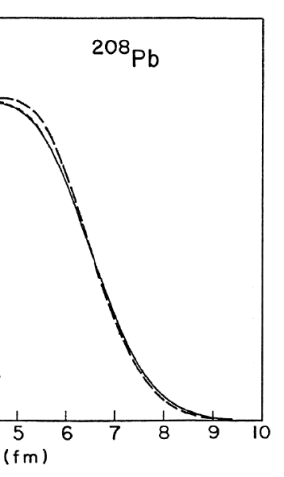
FIG. 5.: The charge density in ²⁰⁸Pb. The dotted and thin dashed curves are mean field calculations with reasonable surface energies while the thick dashed curve is a mean field calculation with a very high surface energy [29]. The experimental charge density is the solid curve.

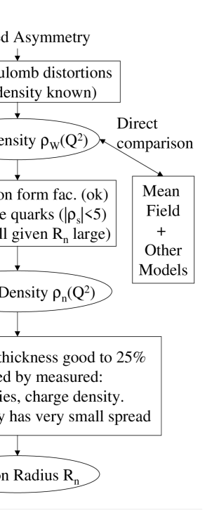
FIG. 6.: Flowchart of the physics data analysis of a neutron radius experiment, see text.

VI Connection to Atomic Parity Nonconservation

Parity violating electron scattering (PVES) measurements of the neutron density will have an important impact on atomic parity nonconservation (PNC) measurements. In the future, the most precise low energy tests of the Standard Model will require a combined knowledge of neutron densities and atomic PNC observables. In this section we discuss the quantitative relationship between PVES and atomic PNC. As an instructive illustration, we use approximate parametrizations of the neutron density and calculate the relative sensitivity of both PVES and atomic PNC to the shape of the nuclear distribution. For both PVES and atomic PNC, these simplified analytical approximations agree well with the more precise numerical solutions[24, 10]. The sensitivity to the neutron distribution shape parameters is found to be approximately the same for PVES and atomic PNC, at the kinematics where PVES is most feasible.

Atomic parity violation experiments can measure the weak charge of a nucleus[9], which at tree level in the Standard Model is $Q_{W}^{St.Mod}=(1-4\sin^{2}\theta_{W})Z-N$. The effect of finite nuclear extent is to modify N and Z to $q_{n}N$ and $q_{p}Z$ respectively[10], where

$$q_{{n}({p})}=\int f(r)\rho_{{n}({p})}(r)d^{3}r.$$ (49)

This nuclear structure correction involves an overlap integral somewhat similar to the weak form factor of Eq. 13, but here $f(r)$ is a $q$-independent folding function determined from the radial dependence of the electron axial transition matrix element inside the nucleus. If the opposite parity atomic states which mix are labelled s and p then $f(r)\propto\psi_{p}^{\dagger}(r)\gamma_{5}\psi_{s}(r)$. We avoid computing the absolute normalization of the electronic wavefunctions, a calculation requiring full many-body atomic wave function correlations, by setting f(0)=1. The approximations we have already made are as follows: We treat the nucleons nonrelativistically, ignoring weak nuclear magnetism effects, and we neglect non-nucleonic degrees of freedom. We neglect terms involving the vector-electron interaction, and thus axial- or anapole- nuclear interactions (Experimentally, this requires properly averaging over hyperfine transitions). The required electron s- and p- wave functions can be computed by solving the single electron Dirac Equation in the presence of the nuclear charge distribution. By doing this, we neglect effects of electron shielding in the vicinity of the nucleus, and the effects of electronic binding energies (and thus many-body correlations) because these are small in comparison with the nuclear Coulomb potential at short (fm) distances. level

Atomic theorists make predictions for atomic observables including a complete many body computation of the axial matrix elements with proper norm[31]. To date, they have generally assumed an isoscalar nuclear density distribution $\rho_{n}(r)=\rho_{p}(r)$, and factored the effect of finite nuclear size into a coefficient of $Q_{W}$. The fact that $\rho_{n}\neq\rho_{p}$ means that there will then be a small additive correction which should be made:

$$Q_{{w}}^{\rm expt}=Q_{{w}}^{\rm St.Mod}+\Delta Q_{{w}}^{{n-p}},$$ (50)

where $Q_{w}^{\rm expt}$ is the weak charge extracted from atomic experiments, using atomic theory calculations which ignore any neutron-proton differences, and to a good approximation,

$$\Delta Q_{{w}}^{{n-p}}=N(1-q_{{n}}/q_{{p}}).$$ (51)

$\Delta Q_{W}^{n-p}$ is zero if neutron and proton distributions are identical. There are additional small corrections[32] to $\Delta Q_{{w}}^{{n-p}}$ arising from Standard Model radiative corrections, as well as additive corrections arising from e.g. internal structure of the nucleon, but these can be safely neglected since $\Delta Q_{{w}}^{{n-p}}$ is itself so small. Given nuclear structure model predictions for $\rho_{p}(r)$ and $\rho_{n}(r)$, the calculation of $f(r)$ and $\Delta Q_{w}^{n-p}$ is reasonably straightforward, requiring a numerical solution of the Dirac Equation in the vicinity of the nucleus. Results from various nuclear structure model distributions for several nuclei are given in Table LABEL:sjptabi, which shows that neutron-proton distribution differences can affect measurements of the weak charge at marginally measurable levels. The model dependent uncertainty in $\Delta Q_{w}^{n-p}$ appears to be comparable to the value itself, and exceeds Standard Model radiative correction uncertainties. This motivates improved knowledge of the neutron distributions, since charge distributions are generally well measured experimentally.

For the specific case of atomic Cs, recent measurements of transition polarizabilities [9], coupled with previous measurements of parity nonconservation (PNC) [8] have significantly reduced uncertainties associated with the extraction of $Q_{{w}}$(Cs). The latest result[9], $Q_{{w}}^{\rm expt}=-72.06(.28)_{\rm expt}\ (.34)_{\rm atomic\ theory}$ is in mild disagreement, at the $2.5\sigma$ level, with the Standard Model prediction of $Q_{{w}}^{\rm St.Mod.}=-73.20(.13)_{\rm theory}$. [32] The experimental number uses input from atomic theory calculations [33, 34] which incorporate finite nuclear size effects, but do not include the modification due to neutron-proton differences, $\Delta Q_{w}^{n-p}$. Using a relatively naive approximation described below we find that, in order to reduce the contribution of nuclear structure uncertainty to below the level of present atomic theory levels, one would need to know the neutron radius to around $\pm$ 6%. To reduce nuclear structure uncertainties well below the level ($\pm 0.13$) of Standard Model radiative correction uncertainties requires knowledge of the neutron radius to around $\pm 2\%$. Due to the more complex nature of the Cs nucleus (e.g. it is not spin 0) it is unlikely that a PVES experiment will measure the neutron radius of Cs directly, but measurement in a nearby nucleus with comparable N/Z (such as Ba) should provide significantly improved confidence in the ability of nuclear structure models to predict neutron radii in general, and hence reduce the nuclear model dependence of these important Standard Model tests.

Precise numerical codes have computed the effect of the neutron density on PVES[24]. It is instructive to recover this result with a simpler analytical approximation, and then to connect this to atomic PNC. To this end we first approximate $f(r)$ and $\Delta Q_{w}^{n-p}$ by assuming a uniform nuclear distribution, i.e. $\rho(r)$ a constant out to some radius $C$. In this case, the nuclear potential energy is just

$$V(r)=(Z\alpha)*\cases{(-3+r^{2}/C_{p}^{2})/2C_{p}&if $r<C_{p}$\cr-1/r&if $r>C_{p}$,\cr}$$ (52)

neglecting small contributions of neutrons to the nuclear charge distribution. The single electron Dirac Equation can be solved in the presence of this potential by expanding in powers of $(Z\alpha)$, making a power series for the Dirac wave functions inside the nucleus. The result is

$$f(r)=1-(Z\alpha)^{2}\left(\textstyle{1\over 2}(r/C_{p})^{2}-\textstyle{1\over 10}(r/C_{p})^{4}+\textstyle{1\over 150}(r/C_{p})^{6}\right)+{\cal O}(Z\alpha)^{4}$$ (53)

One further simplifying approximation can be made, that $\langle r^{2}\rangle_{n}\approx\langle r^{2}\rangle_{p}$, characterizing the difference by a single small parameter,$\langle r^{2}\rangle_{n}/\langle r^{2}\rangle_{p}\equiv 1+\epsilon$. The result, after applying Eq. 49 is

$$q_{{p}}\approx 1-(Z\alpha)^{2}(.26),$$ (54)

$$q_{{n}}\approx 1-(Z\alpha)^{2}(.26+.221\epsilon),$$ (55)

$$\Delta Q_{{w}}^{{n-p}}\approx N(Z\alpha)^{2}(.221\epsilon)/q_{{p}}.$$ (56)

This can be compared with the PVES asymmetry in elastic electron-nucleus scattering for a spin-0 nucleus. In the Born approximation (and in the absence of isospin violation) this asymmetry is given by Eqn. 11 Using the same approximations as above (uniform distributions, $C_{n}\approx C_{p}$) and defining $A^{\rm nom}\equiv A^{0}_{lr}(Q^{2})\left((1-4\sin^{2}\theta_{W})-N/Z\right)$, we find

$${(A-A^{\rm nom})\over A^{\rm nom}} = \left[{\displaystyle-N/Z}\over{\displaystyle(1-4\sin^{2}\theta_{w}-N/Z)}\right]\left({\displaystyle F_{n}(Q^{2})\over{\displaystyle F_{p}(Q^{2})}}-1\right)$$ (57)

$$\approx \left[1.06\right]\epsilon\left(-{3\over 2}+{1\over 2}\displaystyle{(qC_{p})^{2}\sin(qC_{p})\over{(\sin(qC_{p})-(qC_{p})\cos(qC_{p}))}}\right)+{\cal O}(\epsilon^{2})$$ (58)

For extremely small momentum transfer, the expression in large parentheses can be expanded, yielding $-(qC_{p})^{2}/10+{\cal O}(qC_{p})^{4}$. Knowing $C_{n}$ to $\pm$1% means, according to Eq. 56 that the weak charge for lead would have an uncertainty due to neutron structure of $\approx\pm 0.2$, to be compared with $Q_{W}^{\rm St.Mod}=-118.7\pm 0.2\ ({\rm rad.\ corr})$. According to Eq. 58, at q=0.45 fm^-1, measuring $C_{n}$ to 1% requires an asymmetry measurement with errors around the 3% level, in agreement with the numerical results obtained in ref[24].

The approximation scheme described above can be extended to include rough effects of the nuclear shape using the method of Sandars[35], adding a “thin edge” to the uniform distribution, parameterized by a new skin-thickness parameter $\eta$, defined for any arbitrary distribution by

$$\eta={21\langle r^{4}\rangle\over{25\langle r^{2}\rangle^{2}}}-1.$$ (59)

This form is chosen so $\eta=0$ for a uniform distribution. Typically, $\eta_{proton}\approx 0.10$ for a nucleus such as lead. The presence of a thin edge changes all the moments:

$$\langle r^{n}\rangle\approx\displaystyle{3\over{n+3}}C^{n}\left(1+\eta\displaystyle{n(n+3)\over 8}\right),$$ (60)

from which $\langle r^{2}\rangle=C^{2}(3/5)(1+1.25\eta)$ serves to define $C$ for any distribution. Adding such a “thin skin” to the protons, the charge distribution is unchanged except in a small region near C, and our approximation for $f(r)$ is still fairly accurate. The presence of the thin skin does slightly modify the potential inside the nucleus, which in turn modifies $f(r)$ in a well-defined way. Adding a thin skin to the neutrons as well, assuming the difference $\Delta\eta\equiv\eta_{n}-\eta_{p}\ll 1$, Eq. 56 is then modified to

$$\Delta Q_{{w}}^{{n-p}}\approx N(Z\alpha)^{2}.22\left(\epsilon-0.16\Delta\eta\right)/q_{{p}}.$$ (61)

The insensitivity of the atomic observable to higher moments beyond the rms radius is seen from the small relative coefficient of $\Delta\eta$.

To connect to a more familiar measure of skin thickness, consider a Wood-Saxon form for the density, with radius and thickness parameters $c$ and $z$, as given in equation  33. An analytic series expansion as $z/c\rightarrow 0$ gives $\eta\approx\textstyle{4\over 3}\pi^{2}(z^{2}/c^{2})(1-\pi^{2}z^{2}/c^{2})+...$, $\langle r^{2}\rangle=\textstyle{3\over 5}c^{2}(1+\textstyle{7\over 3}\pi^{2}z^{2}/c^{2})$, and $C^{2}\approx c^{2}(1+\textstyle{2\over 3}\pi^{2}z^{2}/c^{2}+\ldots)$ In this way, we could eliminate $\Delta\eta$ in favor of $\epsilon$ and $\Delta z/z$, where e.g. $\Delta z\equiv z_{n}-z_{p}$ is a difference in Wood-Saxon neutron and proton thickness parameters, and as stated above, $\epsilon=\langle r^{2}\rangle_{n}/\langle r^{2}\rangle_{p}-1$. Evaluating $f(r)$ numerically in the presence of this potential using the analytic series expansion for moments and linearizing in $\epsilon$ and $\Delta z$,

$$\Delta Q_{w}^{n-p}(Pb)\approx 10.6\epsilon-.37\Delta z/z,$$ (62)

while for barium

$$\Delta Q_{{w}}^{{n-p}}(Ba)\approx 3.3\epsilon-0.13\Delta z/z.$$ (63)

In these expressions, higher order effects in $(Z\alpha)$, as well as finite surface thickness, have been taken into account numerically. (We use as nominal inputs[36] $c^{Pb}=6.624$, $z^{Pb}=0.549$, $c^{Ba}=5.700$, $z^{Ba}=0.5314$)

The PVES asymmetry also gets modified by a thin skin, and Eq. 58 gets an additional correction term,

$${(A-A^{\rm nom})\over A^{\rm nom}}\approx{\rm Eq}.~{}\ref{asymm}+\left[1.06\right]\Delta\eta\left(\displaystyle{15\over 8}+(qC_{p})^{2}\displaystyle{{qC_{p}\cos(qC_{p})-6\sin(qC_{p})}\over{8(\sin(qC_{p})-(qC_{p})\cos(qC_{p}))}}\right)$$ (64)

(neglecting any ${\cal O}(\eta_{p})$ corrections here.) In the limit of small momentum transfer, the term in large parenthesis goes to $(qC_{p})^{4}/280$. The PVES asymmetry thus becomes completely insensitive to $\Delta\eta$ at small $Q^{2}$, as one would expect, but at larger $Q^{2}$ the surface shape becomes relatively more important. Table LABEL:sjptabii shows the ratio of the coefficients of $\Delta\eta$ to $\epsilon$ in Eq 64 as a function of momentum transfer. (Note that these numbers implicitly incorporate the approximation $\eta_{p}\rightarrow 0$.) Incorporating finite skin thickness with a Wood-Saxon for the nucleon distributions, the asymmetry can be calculated using asymptotic expansion formulas in c and z, and the result linearized in the small quantities $\epsilon$ and $\Delta z$. The resulting formula is not especially illuminating, but the coefficients of this expansion are shown for lead as a function of momentum transfer in Table LABEL:sjptabiii.

Note that there is a unique momentum transfer where the two observables are sensitive to the same linear combination of neutron radius and surface shape. For lead, assuming a thin edge (Table LABEL:sjptabii), and comparing with Eq. 61, this “matchup” is around $q=0.34$ fm^-1. Using the Wood-Saxon form to incorporate the effects of finite skin thickness, and comparing with Eq. 62, the relative coefficients of $\Delta z/z$ and $\epsilon$ are matched for electron scattering and atomic PNC at $q\approx 0.32$ fm^-1. At this kinematics point, a measurement of PVES is “optimized” to provide the direct information desired for the atomic observable. In the absence of other constraints, this would be the optimal momentum transfer for a PVES measurement if the goal is the most direct measurement of atomic weak charge corrections, rather than a desire to extract and measure the details of the neutron shape distribution. Of course, this is only true to the extent that still higher moments (shape differences beyond the simple thin edge approximation) are not important, which is a decent approximation for the atomic observable, but not so good for the PVES asymmetry. A brute force estimate obtained by assuming a generalized three parameter Gaussian form for the nuclear distributions, allowing the 3 parameters to vary but constraining them to produce values of A within some small window of $A^{\rm nom}$, and then calculating the corresponding spread in $\Delta Q_{w}^{n-p}$, we find an optimal q value of $0.32$ fm^-1. (All these results, however, have been calculated at tree level, without Coulomb corrections.)

Another way of understanding the above result is to compare the function multiplying $\rho_{n}(r)$ in the form factor integral of Eq. 13 (i.e. $j_{0}(qr)$) and in the convolution integral of Eq.  49 (i.e. $f(r)$). Since we are not interested in the volume integral of the weak charge density, which is well known, we can subtract both $f(r)$ and $j_{0}(qr)$ from 1, and plot the remainder to study the relative sensitivity to the radius and to the surface thickness. This is shown in figure 7. For $q=0.30$ fm^-1, $1-j_{0}(qr)$ is nearly proportional to $1-f(r)$, and thus at this $Q^{2}$ one is sensitive to the same ratio of surface and radius in a JLAB parity experiment and in an atomic experiment. The curves for $q=0.45$ fm^-1 are also shown, in this case the curves are not identical but are similar enough so much of the error from an unknown surface thickness cancels when comparing the two integrals.

For lead, ignoring the effects of skin thickness, we found above that the rms neutron radius should be known at roughly the $\pm$1% level to ensure that neutron structure uncertainties are smaller than present Standard Model radiative corrections uncertainties (roughly $\pm$0.2, or about $\pm$0.16%, for the weak charge.) Again ignoring thickness, table LABEL:sjptabii shows that this would require e.g. a PVES asymmetry measurement at q=0.45 fm^-1 at the $\pm$3% level. Including the effect of thickness, the linear combination of $\epsilon$ and $\Delta z/z$ required for the weak charge is not quite the same as the linear combination measured in PVES at arbitrary $q$, but a linear error propagation at $q=0.45$ shows that as long as the relative uncertainty in $z_{n}$ is less than $\approx\pm$50%, the additional uncertainty due to including skin thickness is negligible. Thus, a single PVES measurement taken even at a kinematics point which is not perfectly optimized for the atomic observable will still be sufficient to eliminate nuclear structure effects from the atomic observable at levels below present Standard Model uncertainties.

TABLE I.: Nuclear structure model predictions for $\Delta Q_{q}^{n-p}$. HFB stands for Hartree Fock Bogolyubov, Skl stands for a Skyrme “SLy4” parameter set. G1 is a parameterization from a relativistic nuclear model. The Standard Model value and uncertainty are from Ref. [32].

Model	Element	$Q_{w}^{\rm St.Mod}$	$\Delta Q_{w}^{n-p}$
Gogny[37]	Pb	-118.70(0.19)	0.47
HFB-Skl[38]	“	“	0.57
G1 [39]	“	“	1.0
Gogny	Ba	-77.07(.13)	0.14
HFB-Skl	“	“	0.18
G1 [39]	“	“	0.30

TABLE II.: Table of the coefficients occurring in Eq. 64, written in the form $(A-A^{\rm nom})/A^{\rm nom}=c_{1}(\epsilon+c_{2}\Delta\eta)$, as a function of momentum transfer, $q$, for a ²⁰⁸Pb target. ($\epsilon$ measures the n-p rms radius difference, and $\Delta\eta$ measures the n-p surface shape differences) Note that Eq. 64 is derived assuming $\eta_{p}\rightarrow 0$.

q (fm-1)	$c_{1}$	$c_{2}$
0.2	-.21	-.068
0.25	-.33	-.11
0.3	-.50	-.16
0.35	-.72	-.22
0.4	-1.0	-.30
0.45	-1.4	-.40
0.5	-2.1	-.52

TABLE III.: Table of the coefficients $a_{1}$ and $a_{2}$ occurring in the expression $(A-A^{\rm nom})/A^{\rm nom}=a_{1}\epsilon+a_{2}\Delta z/z$, as a function of momentum transfer, $q$, for a ²⁰⁸Pb target. The coefficients of $\epsilon$ do not match those in Table LABEL:sjptabii for two reasons: finite thickness is incorporated here numerically, using the same nominal inputs as for Eq. 62. Also, note that $\Delta z/z$ is itself a function of both $\epsilon$ and $\Delta\eta$.

q (fm-1)	$a_{1}$	$a_{2}$	$a_{2}/a_{1}$
0.2	-.23	.003	-0.013
0.25	-.37	.008	-0.021
0.3	-.56	.017	-0.031
0.35	-.80	.034	-0.042
0.4	-1.1	.064	-0.056
0.45	-1.6	.12	-0.073
0.5	-2.3	.21	-0.094

FIG. 7.: Approximate nuclear weak density $\rho(r)$ for Pb, along with the function multiplying $\rho(r)$ in the integrals for the weak form factor (namely, $j_{0}(qr)$) and in the atomic correction factor $q_{n}$ (namely $f(r)$). In both cases the function is subtracted from one to eliminate the volume integral of the weak charge density. Curves for $1-j_{0}(qr)$ are shown for two different values of $q$ in fm^-1. Note 4.1(1-f(r)) is almost identical to $1-j_{0}(qr)$ for q=0.30fm^-1.

VII Conclusion

With the advent of high quality electron beam facilities such as CEBAF, experiments for accurately measuring the weak density in nuclei through parity violating electron scattering (PVES) are feasible. The measurements are cleanly interpretable, analogous to electromagnetic scattering for measuring the charge distributions in elastic scattering. From parity violating asymmetry measurements in elastic scattering, one can extract the weak density in nuclei after correcting for Coulomb distortions, which have been accurately calculated[24].

By a direct comparison to theory, these measurements test mean field theories and other models that predict the size and shape of nuclei. They therefore can potentially have a fundamental and lasting impact on nuclear physics.

Furthermore, PVES measurements have important implications for atomic parity nonconservation (PNC) experiments which in the future may become the most precise tests of the Standard Model at low energies. We have shown that to a good approximation, sufficient for testing the Standard Model, the dependence on nuclear shape parameters enters the PVES and PNC observables the same way; therefore, the PVES measurements are directly applicable to the interpretation of atomic PNC if measured on the same nucleus.

Measurements of the weak density lead to the neutron density distribution with unprecedented accuracy. As we have discussed in this paper, PVES yield significant improvement in the accuracy of neutron densities compared to hadronic probes or magnetic scattering. We have shown that the corrections due to strange quarks, neutron electric form factors, parity admixtures, dispersion corrections, meson exchange currents, and several other possible effects in realistic experiments are all small. Further, an asymmetry measurement from a heavy nucleus with 3% accuracy will both establish the existence of the neutron skin and characterize its thickness. The neutron skin is an important, qualitative feature of heavy nuclei which has never been cleanly established in a stable nucleus.

REFERENCES

- [1] B. Frois et. al., Phys. Rev. Lett. 38, 152 (1977).
- [2] T.W. Donnelly, J. Dubach and Ingo Sick, Nuc. Phys. A 503 (1989) 589.
- [3] C. Y. Prescott et al., Phys. Lett. 84B, 524 (1979)
- [4] P. A. Souder et al., Phys. Rev. Lett. 65, 694 (1990)
- [5] W. Heil et al., Nucl. Phys. B327, 1 (1989)
- [6] B. Mueller et al., Phys. Rev. Lett. 78, 3824 (1997)
- [7] K. A. Aniol et al., Phys. Rev. Lett. 82, 1096 (1999)
- [8] C. S. Wood et al, Science 275, 1759 (1997).
- [9] S. C. Bennett and C. E. Wieman, Phys. Rev. Lett.82, 2484 (1999).
- [10] S. J. Pollock, E. N. Fortson, and L. Wilets, Phys. Rev. C 46, 2587 (1992), S.J. Pollock and M.C. Welliver, Phys. Lett. B 464, 177 (1999)
- [11] P. Q. Chen and P. Vogel, Phys. Rev. C 48 1392 (1993)
- [12] L.Ray and G.W.Hoffmann, Phys. Rev. C 31, 538 (1985).
- [13] R.J. Furnstahl, Briand D. Serot and Hua-Bin Tang, Nucl. Phys. A615, 441 (1997); R. J. Furnstahl and Briand D. Serot, nucl-th/9911019.
- [14] P. Ring et. al., Nucl. Phys. A624, 349 (1997).
- [15] Patrizia A. Caraveo et. al., ApJ 461, L91 (1996); A. Golden and A. Shearer, astro-ph/9812207.
- [16] F. Walter, S. Wolk and R. Neuhauser, Nature 379, 233 (1996); Bennett Link, Richard I. Epstein and James M. Lattimer, PRL 83, 3362 (1999).
- [17] E.N.Fortson, Y. Pang, and L. Wilets, Phys. Rev. Lett. 65, 2857 (1990).
- [18] B. Alex Brown, Phys. Rev. C58, 220 (1998).
- [19] D. Vretenar, P. Finelli, A. Ventura, G. A. Lalazissis, and P. Ring, Los Alamos preprint nucl-th/9911024.
- [20] J. A. Nolen, Jr. and J. P. Schiffer, Phys. Lett. 29B, 396 (1969), and Annu. Rev. Nucl. Sci. 19, 471 (1969).
- [21] H. J. Korner and J. P. Schiffer, Phys. Rev. Lett. 27 (1971) 1457.
- [22] C. Olmer et. al., Phys. Rev. C 21, 254 (1980)
- [23] J. F. Prewitt and L. E. Wright, Phys. Rev. C9, 2033 (1974).
- [24] C.J. Horowitz, Phys. Rev. C57 (1998) 3430.
- [25] Relativistic optical code RUNT, E. D. Cooper private communication 1997.
- [26] B. C. Clark, private communication 1999.
- [27] B. Povh, Nucl. Phys. A532 (1991) 133.
- [28] See for example, G. Feinberg, Phys. Rev. D12 (1975) 3575.
- [29] C.J. Horowitz and B. D. Serot, Nuc. Phys. A 368 (1981) 503.
- [30] Aage Bohr and Ben R. Motelson, Nuclear Structure Vol. II, Benjamin 1975, p556.
- [31] See e.g. S. A. Blundell, J. Sapirstein, W. R. Johnson, Phys. Rev. D45 1602 (1992), or V. A. Dzuba et al, Phys Lett. A 141, 147 (1989).
- [32] W. Marciano and J. Rosner, Phys. Rev. Lett. 65, 2963 (1990); 68, 898(E) (1992).
- [33] S. A. Blundell, J. Sapirstein, W. R. Johnson, Phys. Rev. D45 1602 (1992).
- [34] V. A. Dzuba et al, Phys Lett. A 141, 147 (1989).
- [35] J. James and P. G. H. Sandars, University of Oxford Preprint.
- [36] C. de Jager et. al, Atomic Data Nuclear Data Tables 14 (1974) 479 (1974), H. DeVries, C. W. DeJager, C. DeVries Atomic Data Nuclear Data Tables, 36 495 (1987)
- [37] J. Decharge, private communication.
- [38] J. Dobaczewski, private communication.
- [39] H. Mueller, private communication.