Low- and Intermediate-Energy Nucleon-Nucleon Interactions and the Analysis of Deuteron Photodisintegration within the Dispersion Relation Technique

Abstract

The nucleon-nucleon interaction in the region of the nucleon kinetic energy up to $1000$ MeV is analysed together with the reaction $\gamma d\to pn$ in the photon energy range $E_{\gamma}=0-400$ MeV. Nine nucleon-nucleon $s$-channel partial amplitudes are reconstructed in the dispersion relation $N/D$ method: ${}^{1}S_{0}$, ${}^{3}S_{1}-^{3}D_{1}$, ${}^{3}P_{0}$, ${}^{1}P_{1}$, ${}^{3}P_{1}$, ${}^{3}P_{2}$, ${}^{1}D_{2}$, ${}^{3}D_{2}$ and ${}^{3}F_{3}$. Correspondingly, the dispersive representation of partial amplitudes $N\Delta\to pn$, $NN^{*}\to pn$ and $NN\pi\to pn$ is given. Basing on that, we have performed parameter-free calculation of the amplitude $\gamma d\to pn$, taking into account: $(i)$ pole diagram, $(ii)$ nucleon-nucleon final-state rescattering $\gamma d\to pn\to pn$, and $(iii)$ inelastic final-state rescatterings $\gamma d\to N\Delta(1232)\to pn$, $\gamma d\to NN^{*}(1400)\to pn$ and $\gamma d\to NN\pi\to pn$. The $\gamma d\to pn$ partial amplitudes for nine above-mentioned channels are found. It is shown that the process $\gamma d\to pn\to pn$ is significant for the waves ${}^{1}S_{0}$, ${}^{3}P_{0}$, ${}^{3}P_{1}$, at $E_{\gamma}=50-100$ MeV, while $\gamma d\to N\Delta\to pn$ for the waves ${}^{3}P_{2}$, ${}^{1}D_{2}$,${}^{3}F_{3}$ dominates at $E_{\gamma}>300$ MeV. Meson exchange current contributions into the deuteron disintegration are estimated: they are significant at $E_{\gamma}=100-400$ MeV.

1 Introduction

Investigations of the lightest nuclei such as deuteron, ${}^{3}He$, ${}^{3}H$, or ${}^{4}He$ were always challenging for researchers. There are at least two reasons for that:
$(i)$ Investigations of simple nuclei give a chance to comprehend better the crucial problems of nuclear physics, such as the structure of nucleon-nucleon forces, the role of multinucleon interactions, the role of internuclear forces at small and large distances, the problem of multiquark bags like $6q$ or $12q$, meson degrees of freedom in nuclei, the role of relativistic effects, etc.
$(ii)$ The study of light nuclei provides an opportunity to elaborate the methods for the description of composite systems. Hadron physics is a physics of composite particles — quarks and gluons being constituents. Elaboration of new approaches for the description of composite systems based on the study of light nuclei has an undoubtful advantage that constituents (nucleons) are observed particles, with known interaction amplitudes.

This paper is devoted to simultaneous investigation of the two two-nucleon processes, namely, $NN\to NN$ at $0\leq T\leq 1000$ MeV and $\gamma d\to pn$ at $0\leq E_{\gamma}\leq 400$ MeV. This simultaneous investigation is not accidental: the $NN\to NN$ amplitude is basic for the study of the two-nucleon reactions. At the same time, the reaction $\gamma d\to pn$ is one of the simplest processes with two nucleons; therefore, the simultaneous analysis should clarify the points:
$(i)$ To what extent and at what energies the nucleon-nucleon interaction governs the other processes induced by this interaction; and
$(ii)$ What characteristics of the nucleon-nucleon interaction play the leading role.

For the deuteron photodisintegration at the photon energies in the laboratory frame $0\leq E_{\gamma}\leq 400$ MeV, numerous experimental data exist, see refs. [1] – [13] and references therein. This region covers both small energies, where quantum mechanics works, and comparatively large energies, where relativistic effects and inelastic processes are important.

The reaction $\gamma d\to pn$ is investigated using dispersive integration technique, which is appropriate for the analysis of partial wave amplitudes:
$(i)$ This technique is relativistic invariant;
$(ii)$ It keeps under control all intermediate states allowing to take properly into account final state rescatterings which are determined by the right-hand singularities of the amplitudes [14]; $(iii)$ In this technique there is no ambiguity related to the mass-off-shell amplitudes.

The dispersion relation technique has much common with both non-relativistic quantum mechanics approach and light-cone variable technique, the methods which are widely used by non-perturbative QCD (or Strong-QCD ). A similarity of the dispersion relation and light-cone variable techniques was specially outlined in ref. [16] where the Perturbative-QCD onset in meson form factors has been analysed.

Consider in more detail the mechanism of the deuteron photodisintegration, $\gamma d\to pn$, at $E_{\gamma}\leq 400$ MeV. The following processes contribute to this reaction: Fig. 1a — the deuteron break-up without nucleon interactions in the final state, Fig. 1b — the deuteron break-up followed by the rescattering of outgoing nucleons, Fig. 1c,d — the photoproduction of one or several mesons in the intermediate state, or — Fig. 1e,f — the photoexcitation of resonances, like $\Delta$ and $N^{*}(1400)$, followed by the transition of the produced particles into the $pn$ state.

We start with the discussion of the nucleon–nucleon interaction. There is a striking property relevant to the hadron interaction at low and intermediate energies: in a wide energy range the nucleon interaction is almost elastic or quasi-elastic (this means an excitation of nucleons into highly located baryon states), i.e. with the energy growth the onset of genuine inelastic processes is delayed. Typical example is given by the deuteron channel ($pn$ scattering in the ${}^{3}S_{1}$ and ${}^{3}D_{1}$ waves) where, though the threshold of the pion production is at $T=290$ MeV, the phase shift analysis indicates that the inelasticity parameter is strongly suppressed up to $T=1000$ MeV [17]. For other waves the inelasticities are related to baryon excitations; for instance, in the ${}^{1}D_{2}$ and ${}^{3}F_{3}$ waves the inelasticities are due to the transitions $NN\to N\Delta(1232)$. The same effect is seen in the pion-pion amplitude, where the inelasticity onset in the $s$-channel, $I=0$, starts at the energy much higher than the four-pion threshold. Presently there is quite a lot of evidences that this is a general feature of the processes at low and intermediate energies: inelasticities are mainly related to the transition of interacting hadron into an excited state, while the prompt production of new quark-antiquark pairs is suppressed. This property being observed several decades ago (see, for example, [18] and references therein) is discussed starting from the early 60’s; it is a foundation of duality ideas and models, such as Veneziano’s model [19].

The direct way to perform a relativistic description of nucleon-nucleon interactions is to use the invariant Feynman technique that leads to the Bethe – Salpeter equation. However, the direct application of the Bethe – Salpeter equation to the nucleon–nucleon interaction faces problems related to mass-off-shell amplitudes and meson production processes. Mass-off-shell phenomena are usually taken into account by the introduction of form factors, that undoubtedly affords an ambiguity in the quantitative representation of the process.

Another problem arises in the description of meson production within the Bethe-Salpeter equation. Indeed, the solution of this equation is represented as a sum of ladder diagrams of the type shown in Fig. 2. The cutting of ladder diagrams defines inelasticities of the amplitude; an example of such a cutting is shown in Fig. 2 by dashed line, it corresponds to the transition $NN\to NN+meson$. The problem is that the forces in the deuteron channel related to the pion exchange are rather significant. Therefore, due to the cuttings of Fig.2 – type, the Bethe — Salpeter equation leads to significant inelasticities which are switched on at invariant energies $\sqrt{s}=2m+m_{\pi},2m+2m_{\pi},$ etc. To suppress the early inelasticities, in line with the suppression of genuine inelastic processes, and at the same time to hold a non-small interaction related to pion-exchange forces, one should take into account other more complicated diagrams, in order 1) to cancel the right-hand $s$-channel singularities with the help of a destructive interference, and 2) to keep the neighbouring $t$-channel singularities (or left-hand ones) that respond to the non-small meson–exchange forces.

Moreover, an exact summation of ladder diagrams is hardly realizable in the realistic case, thus necessary simplifications being induced. One of them consists in the consideration of a potential-type interaction. Another one is an actual replacement of the constituent (nucleon) propagator by its residue $(k^{2}-m^{2})^{-1}\to 2\pi i\theta(k_{0})\delta(k^{2}-m^{2})$ [20]. However, this latter procedure leads to anti-casual singularities of the amplitude; hence, one should take care these singularities be far from the region the approach pretends to describe.

A correct handling of the $s$- and $t$-channel singularities of the amplitude may be performed comparatively easily in the framework of the dispersive N/D method [14], where contributions of the left-hand singularities due to the $t$- and $u$-channel exchanges are independent of the right-hand singularities which are related to the $s$-channel elastic and inelastic processes. An advantage of this technique is its relativistic invariance, together with an absence of a problem of the off-shell amplitude definition. For all intermediate particles, the equality $k^{2}=m^{2}$ is fulfilled, thus allowing us to describe interactions using mass-on-shell amplitudes. Moreover, in the dispersion relation technique there are no principal problems with the description of inelasticities related both to the excited baryons and prompt meson production, because all $s$-channel intermediate states are under control. This means that, when using dispersive integrals, one can take into account certain set of the nearest singularities in due course.

It is also important that the dispersion relation technique allows one to determine the relativistic wave function (or vertex function) of the composite (deuteron-like) system. The description of two-particle composite systems within the framework of the dispersive N/D method was developed in ref. [21], where a Lorentz-covariant amplitude for the two-particle composite system interacting with an external vector field has been written, and ambiguities related to the dispersion relation subtractions have been eliminated basing on the gauge invariance and analyticity requirements. Therefore, while in the Feynman diagrammatic technique the gauge invariance is automatically fulfilled and the interaction amplitude obeys the Ward identity, in the dispersion relation technique these general properties of the theory should be considered as supplementary constraints. This is a necessary payment for treating independently left- and right-hand singularities.

In ref. [21] the dispersion relation analysis of the $pn$ scattering amplitude in the ${}^{3}S_{1}-^{3}D_{1}$ channels has been performed. Basing on the phase shift data, the vertices of the $pn$ scattering in this channel have been constructed together with the deuteron vertex functions which are relativistic analogues of the deuteron wave functions. The use of deuteron wave function obtained in such a way allows to describe well the deuteron form factors up to $Q^{2}=2$ GeV${}^{2}/$c² as well as deuteron binding energy and magnetic and quadrupole moments. A successful description of deuteron properties has been obtained taking properly into account the relativistic effects in the $pn$-component, without including non-nucleonic degrees of freedom into deuteron wave function.

The application of the dispersion relation technique to the description of a deuteron has a long history (see refs. [22]): at the early stage, the deuteron form factor has been considered using the $t$-channel dispersion relation, thus bringing the $t$-channel anomalous singularity into consideration. The recent deuteron description in terms of dispersive integrals [21] is based on the double dispersion representation in the deuteron–mass channels, and it does not require special treatment of anomalous singularities. In this point the technique of ref. [21] is analogous to the non-relativistic wave function technique. The detailed consideration of the composite-particle wave functions in the dispersive technique and its relation to the technique of light-cone variables may be found in refs. [21], [23].

Successful description of the elastic deuteron form factors within the dispersion relation technique, gives rise to the problem of the application of this technique to the other two-nucleon processes, in particular to the deuteron photodisintegration.

The reaction $\gamma d\to pn$ was studied during several decades [24]–[37] in the framework of other techniques, mainly in the quantum mechanical and Feynman diagram approaches. These investigations clarify many features of the reaction, among which — an important role of the meson exchange currents [31] (typical diagrams are shown in Fig. 3).

The analysis of the deuteron photodisintegration in the framework of the dispersion relation technique have been carried out in [38]-[39] starting from small energies, where the contribution of inelastic processes is negligible, with a subsequent increase of the energy. In the present paper we expand the analysis onto the region of the photon energy $E_{\gamma}\simeq 250-400$ MeV, where the production of the lightest baryons, $\Delta(1232)$ and $N^{*}(1400)$, is important.

The investigation of the reaction $\gamma d\to pn$ in the dispersive integral technique complements the investigations carried out within other approaches. This is related to the fact that similar processes from the point of view of their diagrammatic presentation may be treated in different approaches in their own ways. Such an example is provided by meson exchange currents, for in the dispersive technique they come from the contribution of anomalous $t$- and $u$-singularities to the amplitude $\gamma d\to pn$.

The paper is organized as follows.

In Chapter 2 the nucleon-nucleon amplitude is analysed in the framework of the dispersion relation technique in the energy range up to $T=1$ GeV. The aim of this analysis is to restore nucleon-nucleon amplitude vertex functions, which play the role of forces of the quantum mechanics approach. These vertices are used in the next Chapter for the calculation of the final state interaction of nucleons in the deuteron photodisintegration. In Section 2.1 the operator expansion of nucleon-nucleon amplitude in partial waves is done, together with the method of constructing covariant partial wave operators. In Sections 2.2 and 2.3, the dispersion relation N/D method is described: it allows to separate left- and right-hand singularities or, in other words, to single out the interaction forces from the production processes. Here the equation for the partial amplitude is written for the one-channel case when inelastic processes are small, and it is also shown how to present the amplitude using the diagrammatic language. In Section 2.4, basing on the phase shift analysis, the $N/D$ amplitude is restored in the channels ${}^{1}P_{1}$ and ${}^{3}D_{2}$, where inelasticity is small. In Section 2.5, the diagrammatic technique is generalized for the two-channel case. This allows us to include inelasticity into the nucleon-nucleon amplitude and expand our analysis on other waves. The channels ${}^{1}D_{2}$, ${}^{3}P_{2}$ and ${}^{3}F_{3}$ with the inelasticity related to the production of $\Delta(1232)$ are considered here. Basing on the phase shift data in the channels $NN$ and $N\Delta$, the amplitudes are restored for the coupled channels ${}^{1}D_{2}(NN)-^{5}S_{2}(N\Delta)$, ${}^{3}P_{2}(NN)-^{5}P_{2}(N\Delta)$ and ${}^{3}F_{3}(NN)-^{5}P_{3}(N\Delta)$. In Section 2.6 we briefly discuss the waves ${}^{3}S_{1}$ and ${}^{3}D_{1}$: these waves were investigated in detail in ref. [21]. In Section 2.7 the structure of inelasticities in the non-resonance channels ${}^{1}S_{0}$, ${}^{3}P_{0}$ and ${}^{3}P_{1}$ is studied: several mechanisms are considered, such as the production of $\Delta(1232)$, $N^{*}(1440)$ or the $S$-wave $\pi N$ pair. The technique for the calculation of three-particle loop diagrams which are necessary for the description of inelastic processes is discussed in Appendix A, there also the $N$-function parameters are given.

In Chapter 3, within the dispersion relation technique, the amplitude $\gamma d\to pn$ is calculated up to the incident photon energy $E_{\gamma}=400$ MeV. The photodisintegration amplitude is taken as a sum of diagrams shown in Fig. 1. Dashed blocks in Fig. 1b-f correspond to the nucleon final state interaction, which includes elastic–scattering diagrams of Fig. 4a–type and intermediate-state particle production processes of Fig. 4b,c–type. In Section 3.1 the pole diagram of Fig. 1a is written in terms of dispersion relation expression in the deuteron channel. In Section 3.2 final state interaction is calculated for the channels ${}^{1}S_{0}$, ${}^{3}S_{1}-^{3}D_{1}$, ${}^{1}P_{1}$, ${}^{3}P_{0}$, ${}^{3}P_{1}$, ${}^{3}P_{2}$, ${}^{3}D_{2}$, ${}^{1}D_{2}$ and ${}^{3}F_{3}$ taking into account the diagrams of Fig. 4a-type only (i.e. neglecting inelastic rescatterings). Such an approximation allows one to describe the photodisintegration amplitude up to $E_{\gamma}=10$ MeV. In Section 3.3 inelasticities related to the production of $\Delta(1232)$ are included into the final–state channels ${}^{3}P_{2}$, ${}^{1}D_{2}$ and ${}^{3}F_{3}$. Two mechanisms contribute to the intermediate $\Delta$-production: the $\Delta$-production in the final-state nucleon-nucleon interaction block (Fig. 4b) and the prompt $\Delta$-production by photon (Fig. 1e). In Section 3.4 the contribution of inelasticities into $\gamma d\to pn$ is calculated for nucleon–nucleon waves ${}^{1}S_{0}$, ${}^{3}P_{0}$ and ${}^{3}P_{1}$. It is shown that the process $\gamma d\to pn\to X\to pn$, where $X$ is one of inelastic states $(N\pi)_{S}N$, $N^{*}(1400)N$ or $N\Delta$, dominates in these waves. These transitions are important at $E_{\gamma}=50-100$ MeV, while the transition $\gamma d\to N\Delta\to pn$ in the waves ${}^{1}D_{2}$, ${}^{3}P_{2}$ and ${}^{3}F_{3}$, Fig. 1e, is important at $E_{\gamma}\simeq 300-400$ MeV.

The detailed discussion of the results is presented in Chapter 4.

2 Dispersion Relation Representation of Nucleon-Nucleon Scattering Amplitude

2.1 Nucleon- Nucleon Vertex Operators for Partial Amplitudes

Consider the structure of multipole operators for the $NN$ partial scattering amplitudes. There are two ways for the presentation of the amplitude expanded in multipoles. Standard matrix element for the transition $NN\rightarrow NN$ (see Fig. 5a) is as follows:

$$(\bar{\Psi}(p^{\prime}_{1})Q^{b}\Psi(p_{1}))\,(\bar{\Psi}(p^{\prime}_{2})\tilde{Q}^{b}\Psi(p_{2}))\,,$$

where $Q^{b}$ and $\tilde{Q}^{b}$ are multipole operators. However, in the dispersive technique it is more convenient to use charge-conjugated fields:

$$\Psi_{c}(-p^{\prime}_{2})=-\bar{\Psi}(p^{\prime}_{2})C\,,\qquad\bar{\Psi}_{c}(-p_{2})=C{\Psi}(p_{2})\,,$$

where $C$ is charge-conjugation operator. Using the Fierz transformation [40], $\Psi(p_{1})\leftrightarrow\Psi_{c}(p_{2}^{\prime})$, one gets

$$(\bar{\Psi}(p_{1}^{\prime})\tilde{Q}^{b}\Psi_{c}(-p^{\prime}_{2}))\,(\bar{\Psi}_{c}(-p_{2})Q^{b}\Psi(p_{1}))\,,$$

where $Q^{b}$ and $\tilde{Q}^{b}$ is another set of operators corresponding to the ${}^{2S+1}L_{J}$ $NN$ state. The whole amplitude, $A(s,t)$, depends on $s=(p_{1}+p_{2})^{2}$ and $t=(p_{1}-p^{\prime}_{1})^{2}$ and can be represented as a sum of partial amplitudes, $A^{b}(s)$, as follows:

$$A(s,t)=\sum_{b}(\bar{\Psi}(p^{\prime}_{1}){I}_{ij}^{b}\tilde{Q}^{b}_{\mu\nu\cdots}\Psi_{c}(-p^{\prime}_{2}))(\bar{\Psi}_{c}(-p_{2}){I}_{ij}^{b}Q^{b}_{\mu\nu\cdots}\Psi(p_{1}))A^{b}(s)\,.$$

Here $Q^{b}_{\mu\nu\cdots}$ and $\tilde{Q}^{b}_{\mu\nu\cdots}$ are left and right operators of the partial amplitude, $\mu,\nu...$ are indices related to the to the state ${}^{2S+1}L_{J}$, and ${I}_{ij}^{b}$ is isotopic operator. Summation in eq. (2.4) is carried out over the whole set of operators $Q^{b}_{\mu\nu\cdots}$.

Consider the structure of the $Q^{b}_{\mu\nu\cdots}$ operator. For the spin-$\frac{1}{2}$ particles, these operators are constructed using metrical tensor $g_{\mu\nu}$, antisymmetrical tensor $\varepsilon_{\mu\nu\alpha\beta},$ $\gamma$-matrices and momenta $k_{\mu}=\frac{1}{2}(p_{1}-p_{2})_{\mu}$ and $P_{\mu}=(p_{1}+p_{2})_{\mu}$. Let us introduce the tensor $T_{\mu^{\prime}\nu^{\prime}\cdots,\mu\nu\cdots}$ related to the two-nucleon loop diagram:

$$\langle Sp[-(\hat{p}_{1}+m)\tilde{Q}^{b}_{\mu\nu\cdots}(-\hat{p}_{2}+m)Q^{a}_{\mu^{\prime}\nu^{\prime}\cdots}]\rangle=\delta^{ab}T_{\mu^{\prime}\nu^{\prime}\cdots,\mu\nu\cdots}\rho(s).$$

Here $\delta^{ab}$ is the Kronecker tensor, the brackets $\langle\cdots\rangle$ denote the integraging over two-particle phase space, $d\Phi(p_{1},p_{2})$:

$$d\Phi(p_{1},p_{2})=\frac{1}{2}\,\frac{d^{4}p_{1}d^{4}p_{2}}{(2\pi)^{6}}(2\pi)^{4}\delta^{4}(P-p_{1}-p_{2})\delta(m^{2}-p_{1}^{2})\delta(m^{2}-p_{2}^{2}),$$

where

$$\int d\Phi(p_{1},p_{2})=\frac{1}{16\pi}\sqrt{\frac{s-4m^{2}}{s}}\equiv\rho(s)\,.$$

We impose the following normalization constraint:

$$T_{\alpha\beta\cdots,\mu\nu\cdots}T_{\mu^{\prime}\nu^{\prime}\cdots,\alpha\beta\cdots}=T_{\mu^{\prime}\nu^{\prime}\cdots,\mu\nu\cdots}\,.$$

For the states with total angular momenta $J=0,1,2$, the $T$-operators are equal to:

$$\begin{array}[]{cc}J=0:&T=1\,,\\ J=1:&T_{\mu^{\prime},\mu}=g_{\mu^{\prime}\mu}^{\bot}\,,\\ J=2:&T_{\mu^{\prime}\nu^{\prime},\mu\nu}=\frac{1}{2}\left(g_{\mu\mu^{\prime}}^{\bot}g_{\nu\nu^{\prime}}^{\bot}+g_{\mu\nu^{\prime}}^{\bot}g_{\nu\mu^{\prime}}^{\bot}-\frac{2}{3}g_{\mu\nu}^{\bot}g_{\mu^{\prime}\nu^{\prime}}^{\bot}\right)\,,\end{array}$$

where $g_{\mu\nu}^{\bot}=g_{\mu\nu}-P_{\mu}P_{\nu}/s$.

With these requirements, we get the following set of the $pn$ vertex operators for the states ${}^{2S+1}L_{J}$ with isotopic spins $I=0,1$:

$$\begin{array}[]{ccc}{}^{1}S_{0}(I=1):&Q=\frac{1}{\sqrt{2s}}\gamma_{5},&\tilde{Q}=-Q,\\ {}^{3}P_{0}(I=1):&Q=\frac{1}{\sqrt{2(s-4m^{2})}},&\tilde{Q}=Q,\\ {}^{3}S_{1}(I=0):&Q_{\mu}=\frac{1}{\sqrt{2s}}\Gamma_{\mu},&\tilde{Q}_{\mu}=-Q_{\mu},\\ {}^{3}D_{1}(I=0):&Q_{\mu}=\frac{1}{2\sqrt{s}}\left[4k_{\mu}\frac{m+\sqrt{s}}{s-4m^{2}}+\gamma_{\mu}^{\bot}\right],&\tilde{Q}_{\mu}=-Q_{\mu},\\ {}^{1}P_{1}(I=0):&Q_{\mu}=\sqrt{\frac{3}{2s(s-4m^{2})}}\gamma_{5}k_{\mu}^{\bot},&\tilde{Q}_{\mu}=Q_{\mu},\\ {}^{3}P_{1}(I=1):&Q_{\mu}=\sqrt{\frac{3}{s^{2}(s-4m^{2})}}\varepsilon_{\mu\alpha\beta\delta}\gamma_{\alpha}P_{\beta}k_{\delta},&\tilde{Q}_{\mu}=-Q_{\mu},\\ {}^{3}P_{2}(I=1):&Q_{\mu\nu}=\sqrt{\frac{3}{2s(s-4m^{2})}}\left[k_{\mu}^{\bot}\Gamma_{\nu}+k_{\nu}^{\bot}\Gamma_{\mu}-\frac{2}{3}(k^{\bot}\Gamma)g_{\mu\nu}^{\bot}\right],&\tilde{Q}_{\mu\nu}=Q_{\mu\nu},\\ {}^{1}D_{2}(I=1):&Q_{\mu\nu}=\frac{\sqrt{60}}{\sqrt{s}(s-4m^{2})}\gamma_{5}\left[k_{\nu}^{\bot}k_{\mu}^{\bot}-\frac{k^{2}}{3}g_{\mu\nu}^{\bot}\right],&\tilde{Q}_{\mu\nu}=-Q_{\mu\nu},\\ {}^{3}D_{2}(I=0):&Q_{\mu\nu}=\frac{\sqrt{10}}{s(s-4m^{2})}\left[k_{\nu}^{\bot}\varepsilon_{\mu\alpha\beta\delta}\gamma_{\alpha}P_{\beta}k_{\delta}+k_{\mu}^{\bot}\varepsilon_{\nu\alpha\beta\delta}\gamma_{\alpha}P_{\beta}k_{\delta}\right],&\tilde{Q}_{\mu\nu}=Q_{\mu\nu},\\ {}^{3}F_{3}(I=1):&Q_{\mu\nu\chi}=\sqrt{\frac{3}{70s^{2}(s-4m^{2})^{3}}}\end{array}$$

$$\times\left[K_{\mu\nu}^{a}\varepsilon_{abc\chi}\gamma_{b}P_{c}+K_{\nu\chi}^{a}\varepsilon_{abc\mu}\gamma_{b}P_{c}+K_{\chi\mu}^{a}\varepsilon_{abc\nu}\gamma_{b}P_{c}\right],\;\tilde{Q}_{\mu\nu\chi}=Q_{\mu\nu\chi}\,.$$

Here $k_{\mu}^{\bot}=k_{\mu}-(Pk)P_{\mu}/s,\;\;\;$ $\gamma_{\mu}^{\bot}=\gamma_{\mu}-\hat{P}P_{\mu}/s,\;\;\;$ $\Gamma_{\mu}=\gamma_{\mu}^{\bot}-2k_{\mu}^{\bot}/(2m+\sqrt{s})\;\;\;$ and
$K_{\mu\nu\chi}=k_{\mu}k_{\nu}k_{\chi}-\frac{k^{2}}{5}(k_{\mu}g_{\nu\chi}^{\bot}+k_{\nu}g_{\chi\mu}^{\bot}+k_{\chi}g_{\mu\nu}^{\bot}).$ Let us stress that in (2.10) we have introduced left and right operators because the trace (2.5) may be the negative in the technique used: this leads to different left and right operators.

It should be noted that $\Psi_{c}$ and $\Psi$ have opposite parities, so $\bar{\Psi}_{c}\gamma_{5}\Psi$ is a scalar and $\bar{\Psi}_{c}\Psi$ is a pseudoscalar.

For the singlet and triplet isotopic states, the isotopic operators are:

$$I=0:\;\;\;I_{ij}=\frac{\delta_{ij}}{\sqrt{2}},\qquad I=1:\;\;\;\vec{I}_{ij}=\frac{\vec{\tau}_{ij}}{\sqrt{2}},$$

where $\vec{\tau}_{ij}$ are Pauli matrices.

Consider as an example the construction of the operator $Q_{\mu\nu}$ for the ${}^{3}P_{2}$ state: the total momentum $J=2$, so this operator is traceless symmetrical tensor of the second rank constructed of $k^{\perp}_{\mu}$ (the $P$ wave state) and $\Gamma_{\nu}$ (the spin-triplet state). Therefore, the operator for the ${}^{3}P_{2}$ state is proportional to $O_{\mu\nu}=k^{\perp}_{\mu}\Gamma_{\nu}+k^{\perp}_{\nu}\Gamma_{\mu}-\frac{2}{3}(k^{\perp}\Gamma)g^{\perp}_{\mu\nu}$, where $Q_{\mu\nu}=N(s)O_{\mu\nu}$ and $N(s)$ is normalization constant. We have:

$$\langle Sp[-(\hat{p}_{1}+m)\tilde{O}_{\mu\nu}(-\hat{p}_{2}+m)O_{\mu^{\prime}\nu^{\prime}}]\rangle=\frac{2}{3}s(s-4m^{2})T_{\mu\nu,\mu^{\prime}\nu^{\prime}}\rho(s).$$

Therefore, the operator for the ${}^{3}P_{2}$ state is:

$$Q_{\mu\nu}=\sqrt{\frac{3}{2s(s-4m^{2})}}O_{\mu\nu}.$$

Likewise, one can construct vertex operators for all partial amplitudes.

The partial amplitude $A^{b}(s)$ for a fixed state is obtained by projecting the whole amplitude $A(s,t)$ given by (2.4) on this state. Corresponding conjugate operator is as follows:

$$(\bar{\Psi}(p_{1})Q^{b}_{\mu\nu...}\Psi_{c}(-p_{2}))\,(\bar{\Psi}_{c}(-p^{\prime}_{2})\tilde{Q}^{b}_{\mu^{\prime}\nu^{\prime}...}\Psi(p^{\prime}_{1})).$$

Thus, we have:

$$4T_{\mu\nu...\mu^{\prime}\nu^{\prime}...}\rho(s)A^{b}(s)\rho(s)=\int d\Phi(p_{1},p_{2})d\Phi(p^{\prime}_{1},p^{\prime}_{2})$$

$$\times(\bar{\Psi}(p_{1})Q^{b}_{\mu\nu...}\Psi_{c}(-p_{2}))\,A(s,t)\,(\bar{\Psi}_{c}(-p^{\prime}_{2})\tilde{Q}^{b}_{\mu^{\prime}\nu^{\prime}...}\Psi(p^{\prime}_{1})).$$

After performing azimuthal-angle integration, the following expression for $A^{b}(s)$ is obtained:

$$4T_{\mu\nu...\mu^{\prime}\nu^{\prime}...}A^{b}(s)=\int_{-1}^{1}\frac{dz}{2}(\bar{\Psi}(p_{1}){Q}^{b}_{\mu\nu...}\Psi_{c}(-p_{2}))A(s,t)(\bar{\Psi}_{c}(-p^{\prime}_{2})\tilde{Q}^{b}_{\mu^{\prime}\nu^{\prime}...}\Psi(p^{\prime}_{1})),$$

where $z$ is the cosine of the angle between $\vec{p}_{1}$ and $\vec{p}^{\prime}_{1}$ in the center-of-mass system of particles 1 and 2: $z=1+2t/(s-4m^{2})$.

2.2 Left-Hand and Right-Hand Singularities and Unitarity of Partial Amplitudes

In this Section we remind the analytic structure of the amplitude when nucleons interact by pion exchanges ($m_{\pi}$ is pion mass). In this case the amplitude has a pole in the $t$-channel at $t=m_{\pi}^{2}$, as well as threshold singularities at $t=(nm_{\pi})^{2}$ $(n=2,3,...)$. In the $s$-channel the amplitude has a singularity at $s=4m^{2}$ related to nucleon rescattering and branching points $s=(2m+nm_{\pi})^{2}$ related to inelastic channels. For the deuteron channel a bound state with the mass $M$ exists: the amplitude has a pole singuliarity at $s=M^{2}$. The $s$-channel partial amplitudes have the same $s$-channel singuliarities (right-hand ones) that the whole amplitude, $A(s,t)$, has. Besides, partial amplitudes have left-hand singularities which correspond to the $t$- and $u$-channel singuliarities of $A(s,t)$ with branching points $s=4m^{2}-m_{\pi}^{2}n^{2}$ — see Fig. 6. Neglecting inelasticities means that we neglect all right-hand cuts, except for the first one with the branching point at $s=4m^{2}$.

Consider the unitarity of the partial amplitude in the physical region (the upper edge of the elastic cut). One has $SS^{+}=1$ with

$$S={\bf 1}+i(2\pi)^{4}\delta^{4}(p_{1}+p_{2}-p^{\prime}_{1}-p^{\prime}_{2})A(s,t).$$

Using the decomposition of the amplitude (2.4) and equation (2.5), we get the unitarity relation for the partial amplitude:

$$Im\,A^{b}(s)=\rho(s)|A^{b}(s)|^{2}.$$

2.3 One-Channel Scattering in the Diagrammatic Dispersion Relation Technique

According to the $N/D$ method [14], the partial amplitude $A(s)$ can be represented as a ratio of two functions (here and below we omit the index $b$ in the partial $NN$ state):

$$A(s)=\frac{N(s)}{D(s)},$$

with $N(s)$ containing left-hand sinquliarities and $D(s)$ containing right-hand ones only. It follows from the unitarity condition (2.18) that

$$Im\,D(s)=-\rho(s)N(s).$$

The used normalization for $D(s)$ reads: $D(s)\rightarrow 1$ at $s\rightarrow\infty$. It is also assumed that there are no CDD-poles [41] in the amplitude. In this way one gets:

$$D(s)=1-\int_{4m^{2}}^{\infty}\frac{ds^{\prime}}{\pi}\frac{\rho(s^{\prime})N(s^{\prime})}{s^{\prime}-s}=1-B(s).$$

One can restore the $N$-function using experimental data, thus solving the problem of finding an amplitude with correct analytic properties in the vicinity of the point $s=4m^{2}$. However, to describe the nucleon-nucleon system (say, deuteron) which interacts with an external field, it is convenient to introduce vertices, which, in the case of a deuteron, play the role of wave functions [42]. In the simplest case, the vertex function may be defined as follows:

$$G(s)=\sqrt{N(s)}\,.$$

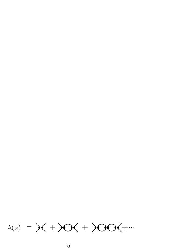
Figure 7: Dispersion relation loop diagrams: (a) representation of the partial amplitude as a set of loop diagrams, (b) one-loop diagram with right ($G_{i}$) and left ($G^{j}$) vertices: $G_{j}B^{i}_{j}G^{i}$.

Then $A(s)$ can be written as a sum of dispersive diagrams shown in Fig. 7a.

$$A(s)=G(s)(1+B(s)+B(s)^{2}+\cdots)G(s),$$

where $B(s)$ corresponds to the one-loop diagram with the vertex $G(s)$.

Consider the one-loop dispersive diagram and its connection with the Feynman one-loop diagram. The Feynman integral reads:

$$A_{F}=\int\frac{d^{4}k}{(2\pi)^{4}i}\frac{a(k^{2}_{1},(P-k_{1})^{2};k^{2},(P-k)^{2})a(k^{2},(P-k)^{2};k^{2}_{2},(P-k_{2})^{2})}{(m^{2}-k^{2})(m^{2}-(P-k)^{2})}.$$

Here $a(k^{2}_{1},(P-k_{1})^{2};k^{2},(P-k)^{2})$ is an irreducible block, without two-particle intermediate states. The receipt for the transition from Feynman integral to the dispersive one is the following. We need:
1) To neglect right-hand multiparticle singularities in the block $a$;
2) To factorize the block $a$:

$$a(k^{2}_{1},(P-k_{1})^{2};k^{2},(P-k)^{2})\to G(k^{2}_{1},(P-k_{1})^{2})G(k^{2},(P-k)^{2});$$

3) To calculate imaginary part of the one-loop Feynman diagram, considering the intermediate state with the energy $\sqrt{s}$ as a real one $(s>4m^{2})$:

$$\frac{d^{4}k}{(2\pi)^{4}i}\frac{1}{(m^{2}-k^{2})(m^{2}-(P-k)^{2})}$$

$$\to\frac{d^{4}k}{(2\pi)^{4}i}\frac{1}{2i}(2\pi i)^{2}\theta(k_{0})\delta(m^{2}-k^{2})\theta(P_{0}-k_{0})\delta(m^{2}-(P-k)^{2})=\rho(s);$$

4) To restore the $B$-function using dispersion relation integral over the imaginary part related to the elastic cut, $disc\,A_{F}$:

$$\int^{\infty}_{4m^{2}}\frac{ds^{\prime}}{\pi}\frac{\rho(s^{\prime})}{s^{\prime}-s}disc\,A_{F}(s^{\prime})=\int^{\infty}_{4m^{2}}\frac{ds^{\prime}}{\pi}\frac{G^{2}(s^{\prime})\rho(s^{\prime})}{s^{\prime}-s}.$$

Finally, we get $G(s)B(s)G(s)$.

The above consideration demonstrates the applicability limit for eq. (2.24): the basic assumption is a factorization of the block $a$.

A general method to perform a factorization of the $t$- and $u$-channel meson exchange interactions has been developed in [42]. For the description of a composite system in general case, one should introduce several vertex functions $G_{i}$ related to a separable interaction $V_{i}$: $N_{i}\rightarrow V_{i}=G_{i}G^{i}$, where the left vertex function, $G_{i}$, and the right one, $G^{i}$, may be different. For further consideration, it is convenient to introduce the amplitudes $a_{i}$ which do not contain the right vertices $G^{i}$. The whole amplitude and auxiliary amplitudes $a_{i}$ are related as:

$$A=\sum_{i}a_{i}G^{i}.$$

The amplitudes $a_{i}$ obey a set of linear equations:

$$a_{i}=\sum_{j}a_{j}B_{i}^{j}+G_{j}\delta_{ij}\,,$$

where (see Fig. 7b)

$$B_{i}^{j}(s)=\int_{4m^{2}}^{\infty}\frac{ds^{\prime}}{\pi}\frac{G^{j}(s^{\prime})\rho(s^{\prime})G_{i}(s^{\prime})}{s^{\prime}-s}\,.$$

Rewriting (2.29) in a matrix form, one has

$$\hat{a}=\hat{B}\hat{a}+\hat{g}\,,$$

where

$$\hat{a}=\left[\begin{array}[]{c}a_{1}\\ a_{2}\\ .\end{array}\right]\,,\quad\hat{g}=\left[\begin{array}[]{c}G^{1}\\ G^{2}\\ .\end{array}\right]\,,\quad\hat{B}=\left[\begin{array}[]{ccc}B_{1}^{1}&B_{1}^{2}&.\\ B_{2}^{1}&B_{2}^{2}&.\\ .&.&.\end{array}\right]\,.$$

The final expression for the partial amplitude reads:

$$A=\hat{g}^{T}(I-B)^{-1}\hat{g}\,,$$

where

$$\hat{g}^{T}=[G_{1},G_{2},\cdots]\,.$$

The amplitude obtained in such a way is unitary; it may be derived from the unitarity condition directly.

Now let us explain how the scattering amplitude discussed above may be written in terms of the energy-off-shell Bethe-Salpeter equation. We need to introduce the energy-off-shell scattering amplitude:

$$A(s,s_{1})=\sum_{i}a_{i}(s)G^{i}(s_{1}).$$

Using equation (2.31), one can write this amplitude as

$$A(s,s_{1})=\int^{\infty}_{4m^{2}}\frac{ds^{\prime}}{\pi}\frac{\rho(s^{\prime})}{s^{\prime}-s}A(s,s^{\prime})V(s^{\prime},s_{1})+V(s,s_{1}).$$

This is a dispersive Bethe-Salpeter equation for $A(s,s_{1})$, where the effective interaction is

$$V(s,s_{1})=\sum_{i}G_{i}(s)G^{i}(s_{1}).$$

The suggested diagrammatic technique is a modification of the standard $N/D$ method: this technique is suitable for the description of an interaction with an external field.

2.4 One-Channel Approach for the Waves ${}^{1}P_{1}$ and ${}^{3}D_{2}$

For the waves ${}^{1}P_{1}$ and ${}^{3}D_{2}$ the inelasticity is small, and corresponding amplitudes can be described in the one-channel approximation. We restore vertex functions of the $pn$ scattering, relying upon the phase shift analysis data [17]. The $G$-function is determined by the left-hand singularities, therefore it is represented as a dispersive integral along the left-hand cuts:

$$G(s)=\int_{-\infty}^{s_{L}}\frac{ds^{\prime}}{\pi}\frac{disc\,G(s^{\prime})}{s-s^{\prime}},$$

where $s_{L}=4m^{2}-m_{\pi}^{2}$ is the location of the nearest pion branching point. Below, to simplify a cumbersome calculation, we replace the integartion in (2.38) by the summation:

$$G_{i}(s)=\sum_{j=1}^{6}\frac{\gamma_{j}^{i}}{s-s_{j}^{i}}\,,\qquad s_{j}^{i}=s_{0}^{i}-h^{i}(j-1),$$

with the poles $s_{j}^{i}$ placed on the left from $s_{L}$.

The values of parameters $\gamma_{j}^{i}$, $h^{i}$ and $s_{0}^{i}$ obtained by fitting the phase shift data are discoursed in Appendix A. The results of the phase shift fit together with the experimental data are demonstrated in Fig. 8.

2.5 Two–Channel Scattering, $NN$ and $N\Delta$:
the Waves ${}^{1}D_{2}$, ${}^{3}P_{2}$ and ${}^{3}F_{3}$

In this Section we consider the inelasticity in the nucleon-nucleon amplitude due to the production of the isobar $\Delta(1232)$. The nucleon-nucleon amplitude is treated as a two-channel one (the channels $NN$ and $N\Delta$). We analyse here the coupled channels: ${}^{1}D_{2}(NN)-^{5}S_{2}(N\Delta)$, ${}^{3}P_{2}(NN)-^{5}P_{2}(N\Delta)$ and ${}^{3}F_{3}(NN)-^{5}P_{3}(N\Delta)$.

Matrix element for the $NN\rightarrow N\Delta$ transition (see Fig. 5b for the momentum notation) is written in the form

$$(\bar{\Psi}^{\mu}(p^{\prime}_{1})\tilde{Q}^{a}_{\alpha\beta,\mu}T_{0}\Psi_{c}(-p^{\prime}_{2}))(\bar{\Psi}_{c}(-p_{2})Q^{b}_{\alpha\beta}{I}\Psi(p_{1}))A^{ab}(s).$$

Here $\tilde{Q}^{a}$ and $Q^{b}$ are vertex operators for the states $a$ and $b$. $T_{\lambda}$ and $I$ are isotopic operators in the $N\Delta$ and $NN$ channels, correspondingly. $A_{ab}(s)$ is the partial amplitude for the transition $state\,b\to state\,a$. $\Psi_{\mu}$ is the wave function for the spin-$\frac{3}{2}$ particle; $\Psi_{\mu}$ obeys the equations:

$$p_{\mu}\Psi_{\mu}(p)=0,\qquad\gamma_{\mu}\Psi_{\mu}(p)=0.$$

For the $N\Delta$ states, vertex operators are as follows:

$${}^{5}S_{2}(N\Delta):\;\;\;\tilde{Q}_{\alpha\beta,\mu}=\frac{1}{\sqrt{\Omega_{1}}}\left[\tilde{\Gamma}_{\alpha}g_{\beta\mu}^{\bot}+\tilde{\Gamma}_{\beta}g_{\alpha\mu}^{\bot}-\frac{2}{3}g_{\alpha\beta}^{\bot}\tilde{\Gamma}_{\mu}\right]\equiv S_{\alpha\beta,\mu},$$

$${}^{5}P_{2}(N\Delta):\;\;\;\tilde{Q}_{\alpha\beta,\mu}=\frac{1}{\sqrt{\Omega_{2}}}\left[\varepsilon_{abc\alpha}k_{a}^{t}P_{b}S_{c\beta,\mu}+\varepsilon_{abc\beta}k_{a}^{t}P_{b}S_{c\alpha,\mu}\right],$$

$${}^{5}P_{3}(N\Delta):\;\;\;\tilde{Q}_{\alpha\beta\gamma,\mu}=\frac{1}{\sqrt{\Omega_{3}}}\left[S_{\alpha\beta,\mu}k_{\gamma}^{t}+S_{\beta\gamma,\mu}k_{\alpha}^{t}+S_{\gamma\alpha,\mu}k_{\beta}^{t}\right.$$

$$\left.-\frac{2}{5}k_{\nu}^{t}(S_{\alpha\nu,\mu}g_{\beta\gamma}^{\bot}+S_{\beta\nu,\mu}g_{\gamma\alpha}^{\bot}+S_{\gamma\nu,\mu}g_{\alpha\beta}^{\bot})\right].$$

Here $\Omega_{i}$ is a normalizing factor; the momenta are defined as $P=p_{1}+p_{2}$, $k=\frac{1}{2}(p_{1}-p_{2})$, $s=P^{2}$, $k^{t}=\frac{1}{2}(p_{1}-p_{2})-\frac{1}{2s}(m_{\Delta}^{2}-m^{2})P$, where $m_{\Delta}$ is the $\Delta$-isobar mass; $k_{\mu}^{\bot}$, $\gamma_{\mu}^{\bot}$ and $g_{\alpha\beta}^{\bot}$ are introduced in Section 2.1, while $\tilde{\Gamma}_{\mu}$ is defined as

$$\tilde{\Gamma}_{\mu}=\gamma_{\mu}^{\bot}-\frac{2k_{\mu}^{\bot}}{m+m_{\Delta}+\sqrt{s}}\,.$$

The $NN$ vertex operators, $Q^{b}$, for ${}^{1}D_{2}$, ${}^{3}P_{2}$ and ${}^{3}F_{3}$ states are given by equation (2.10).

The isotopic operator $T_{0}$ for the states $\Delta^{+}n$ and $\Delta^{0}p$ is defined as

$$T_{0}^{+}=\frac{1}{\sqrt{2}}\left[\begin{array}[]{cc}0&0\\ 1&0\\ 0&1\\ 0&0\end{array}\right]\,,\quad T_{0}=\frac{1}{\sqrt{2}}\left[\begin{array}[]{cccc}0&1&0&0\\ 0&0&1&0\end{array}\right]\,.$$

The partial amplitude $A$ is $2\times 2$ matrix. It is related to the $2\times 2$ $S$-matrix as follows:

$$S=I+2i\sqrt{\rho}A\sqrt{\rho}\,,$$

where $\sqrt{\rho}$ is the matrix of square roots of phase space factors:

$$\sqrt{\rho}=\left[\begin{array}[]{cc}\sqrt{\rho_{NN}}&0\\ 0&\sqrt{\rho_{N\Delta}}\end{array}\right]\,.$$

As before (see Section 2.3), the partial amplitude is represented in the form:

$$A=\hat{g}^{T}(I-\hat{B})^{-1}\hat{g}\,,$$

but with another structure of vertex operators:

$$\hat{g}=\left[\begin{array}[]{cc}G^{N}&0\\ G^{t}&0\\ 0&G^{r}\\ 0&G^{\Delta}\end{array}\right]\,,\qquad\hat{g}^{T}=\left[\begin{array}[]{cccc}G_{N}&0&G_{t}&0\\ 0&G_{r}&0&G_{\Delta}\end{array}\right],$$

and $B$-matrix

$$\hat{B}=\left[\begin{array}[]{cccc}B_{NNN}&0&B_{NNt}&0\\ B_{tNN}&0&B_{tNt}&0\\ 0&B_{r\Delta r}&0&B_{r\Delta\Delta}\\ 0&B_{\Delta\Delta r}&0&B_{\Delta\Delta\Delta}\end{array}\right],\;\;\;B_{ijk}(s)=\int_{T_{j}}^{\infty}\frac{ds^{\prime}}{\pi}\frac{G^{i}(s^{\prime})\rho_{j}(s^{\prime})G_{k}(s^{\prime})}{s-s^{\prime}}\,.$$

Here $G_{N}G^{N}$, $G_{\Delta}G^{\Delta}$, $G_{r}G^{t}$ and $G_{t}G^{r}$ are $N$-functions for the transitions $NN\rightarrow NN$, $N\Delta\rightarrow N\Delta$, $NN\rightarrow N\Delta$ and $N\Delta\rightarrow NN$, correspondingly (see Fig. 5e), $T_{1}=4m^{2}$, $T_{2}=(2m+m_{\pi})^{2}$. In our fit we put $G^{r}=G_{r}$ and $G^{t}=G_{t}$; as it was in previous Section, the two-vertex form is used for the transition $NN\to NN$: $G_{N}G^{N}=G_{1}G^{1}-G_{2}G^{2}$ — Fig. 5f.

For vertex functions the parametrization (2.39) is used. Parameters for $G$ are found using nucleon-nucleon and nucleon-isobar phase shifts, $\delta_{NN}$ and $\delta_{N\Delta}$, and the inelasticity parameter $\eta$ which are defined as

$$S_{11}=\eta e^{2i\delta_{NN}}\;\;,|S_{12}|=|S_{21}|=\sqrt{1-\eta^{2}}\;\;,S_{22}=\eta e^{2i\delta_{N\Delta}}\,.$$

Here indices 1 and 2 refer to the channels $NN$ and $N\Delta$. The description of the phase shift data in the coupled channels ${}^{1}D_{2}-^{5}S_{2}$, ${}^{3}P_{2}-^{5}P_{2}$ and ${}^{3}F_{3}-^{5}P_{3}$ is shown in Fig. 9 together with the experimental data [43].

2.6 Coupled channels ${}^{3}S_{1}$ and ${}^{3}D_{1}$

In Fig. 8 the coupled channels ${}^{3}S_{1}-^{3}D_{1}$ are drawn, for which the inelasticity is small, though the connection of channels is important and the two-channel approach must be applied here [21].

2.7 Models for the Inelasticity in ${}^{1}S_{0}$ wave

According to [17], the mechanism of inelasticity in the waves ${}^{1}S_{0},$ ${}^{3}P_{0}$ and ${}^{3}P_{1}$ differs from the inelasticity in the channels ${}^{1}D_{2}$, ${}^{3}P_{2}$ and ${}^{3}F_{3}$, and the amplitude has a non-resonance behaviour.

Here we consider several models for inelasticity in the ${}^{1}S_{0}$ wave. First, we suggest that the inelasticity comes due to the production of $\Delta(1232)$. Second, we consider as a source of inelasticity the production of $N^{*}_{11}(1440)$. This resonance is heavier than $\Delta(1232)$, but it has larger width, and the transition amplitude ${}^{1}S_{0}(NN)-^{1}S_{0}(NN^{*})$ is not suppressed near the threshold. Third, the prompt pion production in the $\pi N$ $S$-wave is assumed. It should be noted that the 1st and 2nd variants correspond to the production of the $\pi N$-state in the $P$-wave .
1) $\Delta(1232)$-isobar production

Matrix element for the transition ${}^{1}S_{0}(NN)-^{5}D_{0}(N\Delta)$ is determined by (2.40). The vertex operator for the ${}^{5}D_{0}$ wave is

$${}^{5}D_{0}(N\Delta):\;\;\;Q_{\mu}=\frac{1}{\sqrt{\Omega}}\left[\tilde{\Gamma}_{\alpha}g_{\beta\mu}^{\bot}+\tilde{\Gamma}_{\beta}g_{\alpha\mu}^{\bot}-\frac{2}{3}g_{\alpha\beta}^{\bot}\tilde{\Gamma}_{\mu}\right]K_{\alpha\beta}\;\;,\tilde{Q}_{\mu}=-Q_{\mu},$$

where $\Omega$ is the normalization factor and

$$K_{\alpha\beta}=k_{\alpha}^{t}k_{\beta}^{t}-\frac{1}{3}k^{t2}g_{\alpha\beta}^{\bot}\,.$$

The other quantities refer to equations (2.42) and (2.43).
2) Production of $N^{*}(1440)$

Matrix element for the transition $NN\rightarrow NN^{*}$ is written in the form similar to (2.40):

$$(\bar{\Psi}_{N^{*}}(p^{\prime}_{1})\tilde{Q}^{a}I^{i}\Psi_{c}(-p^{\prime}_{2}))(\bar{\Psi}_{c}(-p_{2})Q^{b}I^{i}\Psi(p_{1}))A^{ab}(s)\,.$$

The resonance $N^{*}(1440)$ has the same quantum numbers as a nucleon, so the vertex operator for the $NN^{*}$ state is:

$${}^{1}S_{0}(NN^{*}):\;\;\;Q=\frac{1}{\sqrt{\Omega}}\gamma_{5}\;\;\;,\tilde{Q}=-Q.$$

3) Production of the $(\pi N)_{S}$-pair in the $J^{P}=\frac{1}{2}^{-}$ state

Since the lightest resonances in the $\pi N$ system, with quantum numbers $J^{P}=\frac{1}{2}^{-}$, are located far from the pion-nucleon threshold, we deal here with the case of the prompt non-resonance pion production (Fig. 5c). Nevertheless, we approximate the $\pi N$ pair by a remote quasi-resonance $R$, with an energy–dependent width. This enables us to operate with two-particle intermediate states using the same technique as was used for $\Delta(1232)$ and $N^{*}(1440)$.

Consider the vertex of the quasi-resonance decay $R\to\pi N$: $\Gamma_{\pi}=c_{\pi}\vec{\tau}$. The width of the quasi-resonance $R$, $\Gamma_{R}^{w}$, is defined by its decay into pion and nucleon. This allows us to relate the quantities $c_{\pi}$ and $\Gamma_{R}^{w}$. The resonance propagator is written as:

$$\frac{(\hat{p}+M_{R})}{M_{R}^{2}-p^{2}-B(p^{2})}\,,$$

where $B(p^{2})$ corresponds to the pion–nucleon loop diagram (Fig. 5d). Real part of the loop diagram re-determines the mass of the quasi–resonance $M_{R}$, and imaginary part of $B(p^{2})$ provides its width. Let us rewrite the propagator (2.54) as a series:

$$\frac{(\hat{p}+M_{R})}{M_{R}^{2}-p^{2}-iM_{R}\Gamma_{R}}=\frac{(\hat{p}+M_{R})}{(M_{R}^{2}-p^{2})}+\frac{(\hat{p}+M_{R})}{(M_{R}^{2}-p^{2})}i\Gamma_{R}^{w}M_{R}\frac{1}{(M_{R}^{2}-p^{2})}+...$$

where the first term corresponds to the propagator of a stable particle and the second one to the propagator with the inclusion of the pion-nucleon loop diagram. The Feynman integral for the second term of the right-hand side of eq. (2.55) is equal to:

$$\frac{(\hat{p}+M_{R})}{M_{R}^{2}-p^{2}}\int\frac{d^{4}k}{(2\pi)^{4}i}\frac{c_{\pi}^{2}(\hat{k}+m)}{(m^{2}-k^{2})(m_{\pi}^{2}-(p-k)^{2})}\frac{(\hat{p}+M_{R})}{M_{R}^{2}-p^{2}}\,.$$

The comparison of eqs. (2.55) and (2.56) provides the expression for $\Gamma_{R}^{w}$ in terms of $c^{2}_{\pi}$. To this end, let us decompose $k$ in external vectors $p$ and $k^{\bot}$, the latter being orthogonal to $p$:

$$k=\alpha p+k^{\bot},$$

where $\alpha=(p^{2}+m^{2}-m_{\pi}^{2})/2p^{2}$. The term which is proportinal to $k^{\bot}$ vanishes in eq. (2.56). When comparing eqs. (2.55) and (2.56), it is necessary to calculate imaginary part of the loop diagram and to neglect its real part; for this purpose the following replacement should be done:

$$\frac{1}{(m^{2}-k^{2})(m_{\pi}^{2}-(p-k)^{2}}\rightarrow\frac{1}{2i}(2\pi i)^{2}\delta(m^{2}-k^{2})\theta(k_{0})\delta(m_{\pi}^{2}-(p-k)^{2})\theta(p_{0}-k_{0})\,.$$

Final expression for the width $\Gamma^{w}_{R}$ takes a form:

$$\Gamma^{w}_{R}=\frac{c_{\pi}^{2}}{8\pi M_{R}\sqrt{s}}[(M_{R}+m)^{2}-m_{\pi}^{2}]\left[\frac{(s+m^{2}-m_{\pi}^{2})^{2}}{4s}-m^{2}\right]^{1/2}\,.$$

Vertex operator for the $NR$ system in the ${}^{1}S_{0}$ state is:

$${}^{1}S_{0}(NR):\;\;\;Q=\frac{1}{\sqrt{\Omega}}\,{\bf 1},\;\;\;\tilde{Q}=Q.$$

The description of the $NN$ amplitude is performed within the framework of the two-channel amplitude, where the first channel is the $NN$-state and the second is $N\Delta$, or $NN^{*}$, or $NN\pi$ states, depending on the model we use. The amplitude is restored basing on the phase shift analysis data of ref. [17]. The results of fitting to the phase shift analysis data for the ${}^{1}S_{0}$ wave are shown in Fig. 10a,b. All the three models work equally well in the description of the experimental data on the elastic amplitude $NN\to NN$. However, they provide different results for the amplitude $NN\to NN\pi$.

2.8 $NN^{*}(1400)$ Channel as a Source of Inelasticity in ${}^{3}P_{0}$ and ${}^{3}P_{1}$ Waves

The description of the ${}^{3}P_{0}$ and ${}^{3}P_{1}$ $NN$ waves is performed assuming the production of $N^{*}(1400)$ as a source of inelasticity in the intermediate state. The results of fitting procedure for the ${}^{3}P_{0}$ and ${}^{3}P_{1}$ waves are shown in Fig. 10c-f. Fitting parameters are given in Appendix A.

3 Deuteron Photodisintegration within the Dispersion Relation Technique

In this Section the deuteron photodisintegration amplitude is calculated basing on the analysis performed in the previous Section. This amplitude is represented as a sum of the pole (impulse approximation) diagram (Fig. 1a), diagram with nucleon-nucleon final state interaction (Fig. 1b) and diagrams with the photoproduction of $\Delta(1232)$, $N^{*}(1400)$ and pions in the intermediate state (Fig. 1c-f). It should be stressed that all parameters which are necessary for the calculation of these diagrams have been found in the Section 2, where nucleon – nucleon interaction have been studied; therefore the calculation of the $\gamma d\to pn$ amplitude is parameter-free.

3.1 Pole Diagram

Consider the amplitude $A^{pol}$, which corresponds to the pole diagram of Fig. 11a, written within the dispersion relation technique. We start with the presentation of the Feynman pole diagram:

$$A^{pol}=\xi_{\tau}\varepsilon_{\mu}M_{\tau\mu}^{pol}\,,$$

where

$$M_{\tau\mu}^{pol}=\bar{\Psi}(p_{1})\Gamma_{\mu}\frac{\hat{p}+m}{m^{2}-p^{2}}I^{d}\Gamma_{\tau}^{d}\Psi_{c}(-p_{2})\,.$$

Here $\xi_{\tau}$ and $\varepsilon_{\mu}$ are polarization vectors of the deuteron and photon which are orthogonal to the deuteron and photon, $P\;\;(P^{2}=M^{2})$ and $q\;\;(q^{2}=0)$, momenta:

$$(\xi P)=0\,,\qquad(\varepsilon q)=0\,.$$

The deuteron isotopic operator, $I^{d}(I=0)$, is

$$I_{ij}^{d}=\frac{\delta_{ij}}{\sqrt{2}}\,.$$

Vertex functions for the transition $deuteron\to nucleons$, $\Gamma_{\tau}^{d}$, and for the photon-nucleon interaction, $\Gamma_{\mu}$, are of the form:

$$\Gamma_{\tau}^{d}=\gamma_{\tau}\phi+(p-p_{2})_{\tau}\varphi,\;\;\;\Gamma_{\mu}=e(\gamma_{\mu}f_{1}+(p+p_{1})_{\mu}f_{2})\,,$$

where the vertex functions $f_{1}$ and $f_{2}$ are matrices in the isotopic space:

$$f_{i}=(f_{i}^{p}+f_{i}^{n}){\bf 1}+(f_{i}^{p}-f_{i}^{n}){\bf\tau}_{3}\,.$$

Here ${\bf 1}$ and ${\bf\tau}_{3}$ are isotopic matrices ${\bf 1}=diag(1,1)$ and ${\bf\tau}_{3}=diag(1,-1)$. Indices $p$ and $n$ stand for the photon-proton and photon-neutron form factors; $\phi$, $\varphi$ and $f_{i}^{N}(N=p,n)$ depend on invariant variables.

Consider the transition from the Feynman pole amplitude (3.2) to the dispersion relation one. For this diagram the dispersion relation is written in the deuteron channel, where the pole diagram contains the two-particle threshold only, which corresponds to the production of two nucleons in the intermediate state (in Fig. 11a the relevant two-particle cut is shown by dashed line).

When going from the Feynman amplitude to the dispersive one, the intermediate state vector $\tilde{P}$ should be introduced, see Fig. 11a: $\tilde{P}=p+p_{2}$, $\tilde{P}^{2}=\tilde{s}$. The transition to the dispersive integral in the deuteron channel is carried out at fixed total energy $s=(p_{1}+p_{2})^{2}$. Let us introduce $\tilde{q}=-p+p_{1}$ which satisfies the equations:

$$\tilde{P}+\tilde{q}=p_{1}+p_{2}=P+q.$$

For the calculation of kinematic relations, it is suitable to use the deuteron rest frame, where

$$q=(q_{0},\vec{q}),\;\;\;P=(M,0),\;\;\;\tilde{P}=(\sqrt{\tilde{s}},0),\;\;\;\tilde{q}=(M+q_{0}-\sqrt{\tilde{s}},\vec{q}).$$

One can see that $\tilde{q}^{2}=(p-p_{1})^{2}\neq q^{2}$. This inequality is related to the energy non-conservation in the dispersive integrals. The photon energy in the deuteron rest frame $q_{0}$ is determined by $s$ as:

$$M^{2}+2Mq_{0}=s.$$

We get from (3.9) and (3.10):

$$\tilde{q}^{2}=s+\tilde{s}-\frac{\sqrt{\tilde{s}}}{M}(s+M^{2}).$$

Calculation of the discontinuity in the deuteron channel is equivalent to the replacement of the propagator by the $\delta$-function, considering the two-nucleon intermediate state as a real one:

$$\frac{1}{m^{2}-p^{2}}\rightarrow\frac{1}{2}(2\pi i)\delta(m^{2}-p^{2})\theta(p_{0})\,.$$

Using the discontinuity across the two-nucleon cut, we reconstruct the amplitude

$$M_{\tau\mu}^{pol}=\int_{4m^{2}}^{\infty}\frac{d\tilde{s}}{\tilde{s}-M^{2}}\delta(m^{2}-p^{2})\theta(p_{0})\bar{\Psi}(p_{1})\Gamma_{\mu}(\hat{p}+m)I^{d}\Gamma_{\tau}^{d}(\tilde{s})\Psi_{c}(-p_{2})\,.$$

The substitution (3.11) corresponds to physical decay of the virtual deuteron with momentum $\tilde{P}$ into two nucleons with the on-shell momenta $p$ and $p_{2}$. Rewriting the $\delta$-function argument in the form

$$p^{2}-m^{2}=\tilde{s}-2\tilde{P}p_{2},$$

we elimitate the integration in (3.12):

$$M_{\tau\mu}^{pol}=\frac{2}{\tilde{s}-M^{2}}\bar{\Psi}(p_{1})\Gamma_{\mu}(\hat{\tilde{P}}-\hat{p}_{2}+m)I^{d}\Gamma_{\tau}^{d}\Psi_{c}(-p_{2})\,.$$

In the photon-deuteron center-of-mass frame one has:

$$\tilde{s}=\frac{1}{4}\left(\frac{s+M^{2}}{M}-\sqrt{\frac{s-4m^{2}}{s}}\frac{s-M^{2}}{M}z\right)^{2}\,,z=\cos(\vec{q},\vec{p}_{1})\,,$$

$$\tilde{P}=\sqrt{\frac{\tilde{s}}{s}}\left(\frac{s+M^{2}}{2M}\,,\vec{n}\frac{s-M^{2}}{2M}\right)\,.$$

Let us compare the expressions for the pole diagram provided by the Feynman amplitude and the dispersion relation one. In the deuteron rest frame the denominator of the Feynman amplitude (3.2) is:

$$2(m^{2}-p^{2})=2(2Mp_{20}-M^{2})=2M(2p_{20}-M).$$

Corresponding denominator related to the pole term in the dispersion relation amplitude is equal to:

$$\tilde{s}-M^{2}=4p^{2}_{20}-M^{2}=(2p_{20}+M)(2p_{20}-M).$$

Let us stress that the momentum $p$ is different in both techniques, namely, $p=P-p_{2}$ for the Feynman integral and $p=\tilde{P}-p_{2}$ for the dispersive one and, correspondingly, the functions $\phi,\varphi,f_{1}$ and $f_{2}$ are different too. However, in the non-relativistic limit, $(2p_{20}+M)\simeq 2M$, the dispersive and Feynman pole amplitudes coincide with each other.

Since the intermediate particles in the dispersive technique are mass-on-shell, the functions $\phi$ and $\varphi$ in (3.5) depend on $\tilde{P}^{2}$ only $(\tilde{P}^{2}=\tilde{s})$. Their numerical values are given in [21]. Form factors $f_{1}^{N}$ and $f_{2}^{N}$ depend on $q^{2}$ only.

These functions can be expressed in a standard way in terms of the electric, $f_{e}^{N}$, and magnetic, $f_{m}^{N}$, nucleon form factors:

$$f_{1}^{N}=f_{m}^{N},\;\;\;f_{2}^{N}=\frac{2m}{4m^{2}-q^{2}}(f_{e}^{N}-f_{m}^{N})\,.$$

In equation (3.8) $q^{2}$ is equal to zero.

3.2 Nucleon-Nucleon Final State Interaction

We calculate here the triangle diagram of Fig. 11b, with nucleon–nucleon interactions in the final state. In the triangle diagram the nucleonic degrees of freedom are taken into account only; contribution of non-nucleonic degrees of freedom is considered in the next Section. Although we consider here the one-channel nucleon-nucleon amplitude, the developed method can be easily generalized for the case of multichannel scattering in the final state, such as the scattering in ${}^{3}S_{1}-^{3}D_{1}$ waves.

We classify partial $\gamma d\to pn$ amplitudes according to the final state $pn$-waves ($pn$ system in the state $b$ is determined by (2.4) and (2.33)). The amplitude $\gamma d\to pn$ with the $pn$ final state interaction is written as

$$A_{tr}^{b}=\xi_{\tau}\epsilon_{\mu}M_{\tau\mu}^{b}\,,$$

where

$$M_{\tau\mu}^{b}=\hat{g}^{T}({\bf 1}-B)^{-1}\Delta_{\tau\mu,\alpha^{\prime}\beta^{\prime}}(\bar{\Psi}(p_{1})I_{ij}^{b}\tilde{Q}^{b}_{\alpha\beta}\Psi_{c}(-p_{2}))\,.$$

The amplitude $\Delta_{\tau\mu,\alpha\beta}$ corresponds to the triangle diagram contribution, Fig. 11b, while $M_{\tau\mu}^{b}$ is a sum of graphs with a full set of the final state nucleon rescattering diagrams. Vertex matrix $\hat{g}^{T}$ and loop diagram matrix $B$ are determined by the $pn$ scattering amplitude, see eqs. (2.30) – (2.34). $\Delta_{\tau\mu,\alpha^{\prime}\beta^{\prime}}$ can be written in the form analogous to $\hat{g}$:

$$\Delta_{\tau\mu,\alpha\beta}=\left(\begin{array}[]{c}\Delta_{\tau\mu,\alpha\beta}^{1}\\ \Delta_{\tau\mu,\alpha\beta}^{2}\\ \vdots\end{array}\right)\,.$$

As in the calculation of the pole diagram, we start with the Feynman amplitude for $\Delta_{\tau\mu,\alpha\beta}$:

$$\Delta_{\tau\mu,\alpha\beta}^{i}=\int\frac{d^{4}p^{\prime}_{1}}{(2\pi)^{4}i}\frac{-Sp(\Gamma_{\tau}^{d}I^{d}(\hat{p^{\prime}}+m)\Gamma_{\mu}(\hat{p^{\prime}}_{1}+m)G_{i}Q^{b}_{\alpha\beta}I_{b}(-\hat{p^{\prime}}_{2}+m))}{(m^{2}-p^{\prime 2})(m^{2}-p^{\prime 2}_{1})(m^{2}-p^{\prime 2}_{2})}.$$

After summing over isotopic indices, one gets

$$Sp(I^{d}\Gamma_{\mu}I_{b})=(f_{1}^{p}+(-1)^{I}f_{1}^{n})\gamma_{\mu}+(f_{2}^{p}+(-1)^{I}f_{2}^{n})(p+p_{2})_{\mu}\equiv\tilde{\Gamma}_{\mu}\,.$$

To make a transition from the Feynman amplitude (3.22) to the dispersion relation one, it is necessary to carry out the following steps:

1. To expand the numerator of (3.22) in external four-vectors, for which we choose $P$ and $P_{f}=p_{1}+p_{2}$:

$$-Sp\,(\Gamma_{\tau}^{d}I^{d}(\hat{p^{\prime}}+m)\tilde{\Gamma}_{\mu}(\hat{p^{\prime}}_{1}+m)G_{i}Q^{b}_{\alpha\beta}I^{b}(-\hat{p^{\prime}}_{2}+m))=\sum_{j}d_{j}^{i}F_{\tau\mu,\alpha\beta}^{j}\,.$$

Here $F_{\tau\mu,\alpha\beta}^{j}$ is an expression built up from the vectors $P,P_{f}$ and tensors $g_{\tau\mu},\varepsilon_{\mu\tau\alpha\beta}$. The procedure for constructing invariant functions $d^{i}_{j}$ and the explicit form of $F_{\tau\mu,\alpha\beta}^{j}$ for various $pn$ scattering channels is given in [39].

2. Using (3.24), to represent the expression for $\Delta_{\tau\mu,\alpha\beta}^{i}$ in the form:

$$\Delta_{\tau\mu,\alpha\beta}^{i}=\sum_{j}D_{j}^{i}F_{\tau\mu,\alpha\beta}^{j}\,.$$

For the presentation of $D_{j}^{i}$ as dispersion relation amplitudes, the double discontinuity of the triangle diagram is calculated, i.e. the intermediate two-particle state is considered as a real one, with the neutron-proton energy $\sqrt{\tilde{s}}$ before and $\sqrt{s^{\prime}}$ after the interaction $(\tilde{s},s^{\prime}\geq 4m^{2})$. This procedure corresponds to the replacement:

$$\frac{1}{(m^{2}-p^{\prime 2})(m^{2}-p^{\prime 2}_{1})(m^{2}-p^{\prime 2}_{2})}\rightarrow\frac{1}{4}(2\pi i)^{3}\delta(m^{2}-p^{\prime 2})\theta(p^{\prime}_{0})$$

$$\times\delta(m^{2}-p^{\prime 2}_{1})\theta(p^{\prime}_{10})\delta(m^{2}-p^{\prime 2}_{2})\theta(p^{\prime}_{20})\equiv\rho(\tilde{s},s^{\prime},z)\,.$$

3.To reconstruct the function $D_{j}^{i}$ using the dispersion integral with a double discontinuity as an integrand, :

$$D_{j}^{i}=\int_{4m^{2}}^{\infty}\frac{d\tilde{s}\,\,ds^{\prime}}{\pi^{2}}\frac{disc\,\,disc\,D_{j}^{i}}{(\tilde{s}-M^{2})(s^{\prime}-s)}\,.$$

Here

$$disc\,\,discD_{j}^{i}=\int\frac{d^{4}p_{1}}{(2\pi)^{4}}\rho(\tilde{s},s^{\prime},z)d_{j}^{i}(\tilde{s},s^{\prime},z)\,.$$

Using the results obtained by the derivation of (3.14), we perform integration over $s$ in (3.27). This gives:

$$D_{j}^{i}=\int\frac{ds^{\prime}}{\pi}\int_{-1}^{1}\frac{dz}{2}\rho(s^{\prime})\frac{2d_{j}^{i}(\tilde{s},s^{\prime},z)}{(\tilde{s}-M^{2})(s^{\prime}-s)}\,.$$

$\rho(s^{\prime})$ is given by (2.7), $\tilde{s}$ is defined according to (3.15), $s=P_{f}^{2}$, $z=\cos(\vec{q},\vec{p^{\prime}}_{1})$. Invariant functions $D_{j}^{i}$ determine the function $\Delta_{\tau\mu,\alpha\beta}$ (3.25) and, consequently, the amplitude $M^{b}_{\tau\mu}$.

3.3 Photodisintegration Amplitude with $\Delta(1232)$ in the Intermediate State

In this Section we include into the photodisintegration amplitude the $\Delta$-isobar produced in the intermediate state. The importance of an isobar in the deuteron photodisintegration was emphasized in numerous papers (see, for example, [33],[34],[36]). The isobar reveals itself in two ways:
1) As an $N\Delta$ intermediate state in the final state nucleon-nucleon rescatterings (dashed block in Fig. 1b,c);
2) In the prompt photoproduction, with a subsequent transition $N\Delta\to pn$ in the triangle diagrams of Fig. 1e-type.

Here we calculate the photodisintegration amplitude with $N\Delta(1232)$ in the intermediate state, taking into account the coupled channels ${}^{1}D_{2}(NN)$ $-^{5}S_{2}(N\Delta)$, ${}^{3}P_{2}(NN)$ $-^{5}P_{2}(N\Delta),$ and ${}^{3}F_{3}(NN)$ $-^{5}P_{3}(N\Delta)$.

1) $\Delta$-isobar, $\gamma N$ partial width and the coupling

We start the treatment of $\Delta(1232)$ in the deuteron photoproduction amplitude with a consideration of the transition coupling for $N\gamma\rightarrow\Delta$, which determines the process of Fig. 1e. The propagator of the stable $\Delta$-isobar, with mass $m_{\Delta}$, is equal to

$$\frac{(\hat{p}+m_{\Delta})(-g_{\alpha\beta}^{\bot}+\frac{1}{3}\gamma_{\alpha}^{\bot}\gamma_{\beta}^{\bot})}{m_{\Delta}^{2}-p^{2}}\,.$$

Re-definition of the propagator for the case of a decay into nucleon and photon consits in a replacement:

$$(m_{\Delta}^{2}-p^{2})^{-1}\rightarrow(m_{\Delta}^{2}-p^{2}-B_{\gamma}(p^{2}))^{-1}\,,$$

where $B_{\gamma}(p^{2})$ is the photon–nucleon loop diagram. The real part of this diagram re-determines $m_{\Delta}$, and the imaginary part of $B_{\gamma}(p^{2})$ gives the partial width $\Gamma^{w}_{\gamma}$ for the decay $\Delta\to\gamma N$:

$$\frac{(\hat{p}+m_{\Delta})(-g_{\alpha\beta}^{\bot}+\frac{1}{3}\gamma_{\alpha}^{\bot}\gamma_{\beta}^{\bot})}{m_{\Delta}^{2}-p^{2}-im_{\Delta}\Gamma^{w}_{\gamma}(p^{2})}\,.$$

Thus, we have to calculate $B_{\gamma}(p)$. The following expression stands for the $\Delta$-isobar propagator with $B_{\gamma}(p)$ considered as a perturbative correction:

$$\frac{(\hat{p}+m_{\Delta})(-g_{\alpha^{\prime}\beta}^{\bot}+\frac{1}{3}\gamma_{\alpha^{\prime}}^{\bot}\gamma_{\beta}^{\bot})}{m^{2}_{\Delta}-p^{2}}\int\frac{d^{4}q}{(2\pi)^{4}i}\,\Gamma_{\alpha\mu}^{\Delta}\,\frac{(\hat{k}+m)}{m^{2}-k^{2}}\,\Gamma_{\beta\mu^{\prime}}^{\Delta}\,\frac{g_{\mu\mu^{\prime}}}{-q^{2}}$$

$$\times\frac{(\hat{p}+m_{\Delta})(-g_{\alpha\beta^{\prime}}^{\bot}+\frac{1}{3}\gamma_{\alpha}^{\bot}\gamma_{\beta^{\prime}}^{\bot})}{m_{\Delta}^{2}-p^{2}}\,.$$

The vertex operator $\Gamma_{\alpha\mu}^{\Delta}$ has the form [46]:

$$\Gamma_{\alpha\mu}^{\Delta}=c_{\gamma}\gamma_{5}(\hat{q}g_{\mu\alpha}-q_{\alpha}\gamma_{\mu})\sqrt{2}T_{0}\,.$$

Let us decompose the vectors $k$ and $q$ over vectors $p$ and $k^{\bot}$ ($k^{\bot}$ is orthogonal to $p$):

$$q=Ap+k^{\bot}\,,\qquad k=Bp-k^{\bot}\,,$$

where

$$A=\frac{p^{2}-m_{\Delta}^{2}}{2p^{2}}\,,\qquad B=\frac{p^{2}+m_{\Delta}^{2}}{2p^{2}}\,.$$

To calculate the imaginary part of (3.33) the following replacement should be made:

$$\frac{1}{(-q^{2})(m^{2}-k^{2})}\rightarrow\frac{1}{2}(2\pi i)^{2}\delta(m^{2}-k^{2})\theta(k_{0})\delta(-q^{2})\theta(q_{0})\,.$$

When integrating over $k^{\bot}$, the terms proportional to $k^{\bot}$ and $k^{\bot 3}$ vanish, while the quadratic terms should be replaced as follows:

$$k_{\alpha}^{\bot}k_{\beta}^{\bot}\rightarrow\frac{1}{3}\left[-\frac{(p^{2}-m^{2})}{4p^{2}}\right]g_{\alpha\beta}^{\bot}=\frac{1}{3}k_{\bot}^{2}g_{\alpha\beta}^{\bot}\,.$$

Using the equality

$$\left(-g_{\alpha\beta}^{\bot}+\frac{1}{3}\gamma_{\alpha}^{\bot}\gamma_{\beta}^{\bot}\right)\left(-g_{\beta\varepsilon}^{\bot}+\frac{1}{3}\gamma_{\beta}^{\bot}\gamma_{\varepsilon}^{\bot}\right)=\left(-g_{\alpha\varepsilon}^{\bot}+\frac{1}{3}\gamma_{\alpha}^{\bot}\gamma_{\varepsilon}^{\bot}\right)\,.$$

one obtains:

$$\frac{(\hat{p}+m_{\Delta})\left(-g_{\alpha^{\prime}\beta^{\prime}}^{\bot}+\frac{1}{3}\gamma_{\alpha^{\prime}}^{\bot}\gamma_{\beta^{\prime}}^{\bot}\right)}{m_{\Delta}^{2}-p^{2}}\hat{p}\left(A^{2}Bp^{2}-\frac{2}{3}Ak_{\bot}^{2}-\frac{1}{3}Bk_{\bot}^{2}\right)$$

$$\times\,i\frac{p^{2}-m^{2}}{16\pi m_{\Delta}p^{1/2}}\,c_{\gamma}^{2}\,.$$

Fixing $p^{2}=m_{\Delta}^{2}$ in the numerator, we have for the width $\Gamma^{w}_{\gamma}$:

$$\Gamma^{w}_{\gamma}=\frac{1}{8\pi}\left(\frac{m_{\Delta}^{2}-m^{2}}{2m_{\Delta}}\right)^{3}\frac{2m_{\Delta}^{2}+\frac{2}{3}m^{2}}{m_{\Delta}^{2}}\,c_{\gamma}^{2}\,.$$

After presenting $c_{\gamma}$ as $c_{\gamma}=(e/m_{\pi})C$, we get $C=0.30$ (at $\Gamma^{w}_{\gamma}/\Gamma^{w}_{tot}=0.006$ and $\Gamma^{w}_{tot}=115$ MeV), in accordance with refs. [47] and [34].

2) $pn$-production in the waves ${}^{1}D_{2}(NN)$, ${}^{3}P_{2}(NN)$ and ${}^{3}F_{3}(NN)$

The amplitude of the process $\gamma d\to pn$ is given by eq. (3.20). For the waves ${}^{1}D_{2}(NN)$, ${}^{3}P_{2}(NN)$ and ${}^{3}F_{3}(NN)$), the structure of the triangle diagram $\hat{\Delta}_{\tau\mu,\alpha\beta}$ is the same as $\hat{g}$ (which is given by (2.48)), namely:

$$\hat{\Delta}=\left[\begin{array}[]{cc}\Delta^{N}&0\\ \Delta^{t}&0\\ 0&\tilde{\Delta}^{r}\\ 0&\tilde{\Delta}^{\Delta}\end{array}\right]\,.$$

We have two types of triangle diagrams: with nucleons in the intermediate state, $\Delta^{N}$ and $\Delta^{t}$ (Fig. 11b), and with $N\Delta$ intermediate state, $\tilde{\Delta}^{r}$ and $\tilde{\Delta}^{\Delta}$ (Fig. 11c). The calculation of $\Delta^{i}$ is given in Section 3.2. The scheme of calculation of $\tilde{\Delta}^{i}$ is presented below. The Feynman integral corresponding to the diagram of Fig. 11c is:

$$\tilde{\Delta}_{\tau\mu,\alpha\beta}^{i}=\int\frac{d^{4}p^{\prime}_{1}}{(2\pi)^{4}i}\frac{-Sp(\Gamma_{\tau}^{d}\tilde{I}^{d}(\hat{p^{\prime}}+m)\Gamma_{\mu\varepsilon}^{\Delta}(\hat{p^{\prime}}_{1}+m_{\Delta})\tilde{P}_{\varepsilon\varepsilon^{\prime}}G_{i}Q^{a}_{\alpha\beta,\varepsilon^{\prime}}T_{0}(-\hat{p^{\prime}}_{2}+m))}{(m^{2}-p^{\prime 2})(m_{\Delta}^{2}-p^{\prime 2}_{1})(m^{2}-p^{\prime 2}_{2})}\,,$$

where $\Gamma_{\mu\varepsilon}^{\Delta}$ is the vertex for the $\Delta$- photoproduction (3.34). The spin-dependent numerator of the isobar propagator $\tilde{P}_{\varepsilon\varepsilon^{\prime}}$ is:

$$\tilde{P}_{\varepsilon\varepsilon^{\prime}}=-g_{\varepsilon\varepsilon^{\prime}}^{\bot}+\frac{1}{3}\gamma_{\varepsilon}^{\bot}\gamma_{\varepsilon^{\prime}}^{\bot}\,,$$

where

$$g_{\varepsilon\varepsilon^{\prime}}^{\bot}=g_{\varepsilon\varepsilon^{\prime}}-\frac{p^{\prime}_{1\varepsilon}p^{\prime}_{1\varepsilon^{\prime}}}{p^{\prime 2}_{1}}\,,\qquad\gamma_{\varepsilon}^{\bot}=\gamma_{\varepsilon}-\frac{\hat{p^{\prime}}_{1}p^{\prime}_{1\varepsilon}}{p^{\prime 2}_{1}}\,.$$

The expression (3.41) is written for a stable isobar. In the case of an unstable isobar decaying into pion and nucleon, the pole term should be replaced as:

$$(m_{\Delta}^{2}-p^{\prime 2}_{1})^{-1}\rightarrow(m_{\Delta}^{2}-p^{\prime 2}_{1}-B_{\pi}(p^{\prime 2}_{1}))^{-1}\,,$$

where the function $B_{\pi}(p^{\prime 2}_{1})$ is determined by the pion–nucleon loop diagram. The real part of this diagram re-determines the mass, and the imaginary part gives the width $\Gamma^{w}_{\pi}$ of the decay $\Delta\rightarrow N\pi$:

$$Im\,B_{\pi}(p^{\prime 2}_{1})=m_{\Delta}\Gamma^{w}_{\pi}(p^{\prime 2}_{1})\,.$$

Using the Lehman representation, the isobar propagator can be written as follows:

$$(m_{\Delta}^{2}-p^{\prime 2}_{1}-im_{\Delta}\Gamma^{w}_{\pi}(p^{\prime 2}_{1}))^{-1}=\int_{(m+m_{\pi})^{2}}^{\infty}\frac{d\tilde{m}^{2}R(\tilde{m}^{2})}{\tilde{m}^{2}-p^{\prime 2}_{1}-i0}\,,$$

where the weight function, $R(\tilde{m}^{2})$, has the form:

$$R(\tilde{m}^{2})=\frac{1}{\pi}\frac{m_{\Delta}\Gamma^{w}_{\pi}(\tilde{m}^{2})}{(m_{\Delta}^{2}-\tilde{m}^{2})^{2}+(m_{\Delta}\Gamma^{w}_{\pi}(\tilde{m}^{2}))^{2}}\,.$$

Below we accept $\Gamma^{w}_{\pi}=\Gamma^{w}_{tot}$, and the parametrization of ref. [33] is used for the momentum-dependent width:

$$\Gamma^{w}_{\pi}(\tilde{m}^{2})=\Gamma^{w}_{tot}\frac{\tilde{X}^{3}/(1+\tilde{X}^{2})}{X^{3}_{\Delta}/(1+X_{\Delta}^{2})}\,,$$

Here $\tilde{X}=\tilde{q}r/m_{\pi}$, $X_{\Delta}=q_{\Delta}r/m_{\pi}$ with r=0.081, $\tilde{q}$ and $q_{\Delta}$ are pion momenta in the isobar center-of-mass frame for the isobar masses $\tilde{m}$ and $m_{\Delta}$, correspondingly.

Transition from the Feynman amplitude (3.41) to the dispersion relation one makes it necessary to follow the prescription given in Section 3.2. Then we get for $D^{i}_{j}$:

$$D_{j}^{i}=\int_{(m+m_{\pi})^{2}}^{\infty}d\tilde{m}^{2}R(\tilde{m}^{2})\int_{(m+\tilde{m})^{2}}^{\infty}\frac{ds^{\prime}}{\pi}\int_{-1}^{1}\frac{dz}{2}\frac{2d_{j}^{i}}{(\tilde{s}-M^{2})(s^{\prime}-s_{f})}\times$$

$$\times\left(\frac{(s^{\prime}-(\tilde{m}+m)^{2})(s^{\prime}-(\tilde{m}-m)^{2})}{s^{\prime 2}}\right)^{1/2}\frac{1}{16\pi}\,.$$

3.4 Deuteron Photodisintegration and Inelasticities in the Final State Waves ${}^{1}S_{0}$, ${}^{3}P_{0}$ and ${}^{3}P_{1}$

In Section 2.7-2.8 the description of the $NN$ scattering in the waves ${}^{1}S_{0},$ ${}^{3}P_{0}$ and ${}^{3}P_{1}$ has been done, and three different models for the mechanism of inelasticity being suggested: production of $\Delta(1232)$, $N^{*}(1440)$, or $(\pi N)_{S}$-pair. It is shown in Appendix A that the transition amplitude $NN\rightarrow NN$ does not depend on the model used for the inelasticity, i.e. on the type of the transition amplitude $NN\rightarrow NR$, $NR\rightarrow NN$ and $NR\rightarrow NR$, where $R=\Delta$, $N^{*}$, or $(\pi N)_{S}$.

This means that the process of Fig. 1b does not depend on the inelasticity type as well, and it may be calculated within the technique presented in Section 2. However, the processes of Fig.1 c,e,f, with a prompt photoproduction of a resonance or pion – nucleon pair, may depend on the inelasticity type. For the calculation of processes of Fig. 1c,e,f, it is necessary to know the resonance photoproduction amplitudes. It should be noted that $N^{*}(1400)$ has an about 50$\%$ branching rate into the channel $N\pi\pi$, so the triangle diagram with $N^{*}(1400)$ in the intermediate state effectively describes the process of Fig. 1d.

1) Triangle diagram with $N\Delta$ intermediate state

The vertex $\gamma N\to\Delta$ has been presented in Section 3.3. The calculation of triangle diagram with $N\Delta$ intermediate state is carried out in the same way as for the waves considered in previous Section.

2) Triangle diagram with $NN^{*}(1400)$ intermediate state

The resonance $N^{*}(1440)$ has the same quantum numbers as a nucleon, $J^{p}=\frac{1}{2}^{+}$, and the vertex function $F_{\gamma}$ for the transition $N\gamma\rightarrow N^{*}$ is equal to:

$$\Gamma_{\mu}^{N^{*}}=c_{\gamma}\gamma_{\mu}\tau_{3}\,,$$

with the following relation between $c_{\gamma}$ and the width $\Gamma_{\gamma}^{w}$of the decay $N^{*}\to\gamma N$:

$$\Gamma_{\gamma}^{w}M_{N^{*}}=c_{\gamma}^{2}\frac{2(M_{N^{*}}-m)^{2}}{16\pi M_{N^{*}}^{2}}(M_{N^{*}}^{2}-m^{2})\,.$$

The correlation between $\Gamma_{\gamma}^{w}$ and $c_{\gamma}$ may be found in the same way as it has been done in previous Section for $\Delta(1232)$. To define $c_{\gamma}$, we rely upon the fact that the total width of $N^{*}$ is equal to $\Gamma_{tot}=200$ MeV. Let the ratio $\Gamma^{w}_{\gamma}/\Gamma^{w}_{tot}$ be the same for $p\gamma$ and $n\gamma$ channels, being equal to 0.10% [47]. Using (3.46), we get $c_{\gamma}=0.3$. Experimental data [47] on $N^{*}$ do not allow to define the coupling with a high accuracy.

3) Triangle diagram with $N(\pi N)_{S}$ intermediate state

Following the model presented in Section 2.7, we approximate a pion-nucleon pair by the quasi-resonance $R$. Then the vertex function for the transition $\gamma N\rightarrow R$ can be written in the form:

$$\Gamma^{R}_{\mu}=c^{R}_{\gamma}\gamma_{\mu}\gamma_{5}\tau_{3}\,.$$

The coupling $c^{R}_{\gamma}$ is found by calculating the $\gamma p\rightarrow\pi^{+}n$ cross section:

$$\sigma(\gamma p\rightarrow\pi^{+}n)=\int_{-1}^{1}dz\frac{1}{4J}\frac{1}{16\pi s_{\gamma p}}[(s_{\gamma p}-(m_{\pi}^{2}+m^{2}))^{2}-4m^{2}m_{\pi}^{2}]^{1/2}$$

$$\times\frac{c_{\pi}^{2}c_{\gamma}^{2}}{(M_{R}^{2}-s_{\gamma p})^{2}+M_{R}^{2}\Gamma_{R}^{w\,2}}g_{\mu\mu^{\prime}}^{\bot\bot}Sp\{(\hat{k}+m)\gamma_{\mu}\gamma_{5}(\hat{k}+\hat{k}_{\pi}+M_{R})\,$$

$$\times(\hat{k}+m)\gamma_{\mu^{\prime}}\gamma_{5}(\hat{k}+\hat{k}_{\pi}+M_{R})\}\frac{2}{3}\,,$$

where $q$ and $k$ are photon and neutron momenta, $s_{\gamma p}$ is the $\gamma p$ energy squared, and

$$J=2(s-m^{2})\,,\quad g_{\mu\mu^{\prime}}^{\bot\bot}=g_{\mu\mu^{\prime}}-\frac{k_{\mu}k_{\mu^{\prime}}}{k^{2}}-\frac{q_{\mu}^{\bot}q_{\mu^{\prime}}^{\bot}}{q^{\bot 2}}\,,\quad q_{\mu}^{\bot}=q_{\mu}-k_{\mu}\frac{(qk)}{m^{2}}\,.$$

The parameters $c_{\pi}$, $M_{R}$ and $\Gamma_{R}$ standing for the quasi-resonance are introduced in Section 2.7. According to [48], the $\gamma p\rightarrow\pi^{+}n$ cross section has a resonance pick related to the $\Delta$-isobar and a smooth background. We relate this background to the quasi resonance production of the $(\pi N)_{S}$-pair. The quasi-resonance width $\Gamma_{R}^{w}$ is calculated with the simplest ansatz about the vertex of the decay $R\rightarrow\pi N$:

$$\Gamma_{\pi}=c_{\pi}\vec{\tau}\,.$$

The fit provides the following parameters $c_{\gamma}=0.5$, $c_{\pi}=0.7$, $M_{R}=1.85$ GeV.

For all considered waves (${}^{1}S_{0}$, ${}^{3}P_{0}$ and ${}^{3}P_{1}$) and for all types of the models, the result is the following: processes with inelastic production in the triangle-graph intermediate state provide small contribution, in other words, the contribution of diagrams 1c, 1e and 1f is not large, while the main one comes from the diagram of Fig. 1b. For example, the maximum value of the triangle graph contribution in the wave ${}^{1}S_{0}$ comes at $E_{\gamma}=30-50$ MeV, and it does not exceed 5% of $\sigma(^{1}S_{0})$ (see below).

4 Results and Discussion

4.1 Polarization Averaging and Cross Section Calculations

Within the used normalization, the differential unpolarized cross section has the form:

$$d\sigma=\frac{|{A}|^{2}}{J}d\Phi\,,$$

where ${A}$ is the whole disintegration amplitude, which is built up of the amplitude $A=A^{pole}+\sum_{b}A^{b}_{tr}$ by averaging over the spins of incident particles and summed over spins of final particles. The summation $\sum_{b}$ is performed over all considered states ${}^{1}S_{0}$, ${}^{3}S_{1}-^{3}D_{1}$, ${}^{3}P_{0}$, ${}^{1}P_{1}$, ${}^{3}P_{1}$, ${}^{3}P_{2}$, ${}^{1}D_{2}$, ${}^{3}D_{2}$ and ${}^{3}F_{3}$.

The two-particle phase space factor, $d\Phi$, and the flux factor $J$ are defined as:

$$d\Phi=\frac{d^{4}p_{1}d^{4}p^{2}}{(2\pi)^{6}}(2\pi)^{4}\delta^{4}(P-p_{1}-p_{2})\delta(m^{2}-p_{1}^{2})\delta(m^{2}-p_{2}^{2})\,,$$

$$J=4((Pq)^{2}-m^{4})^{1/2}\,.$$

For non-polarized deuteron we need to make the replacement:

$$\xi_{\tau}\xi_{\tau^{\prime}}\rightarrow-\frac{1}{3}g_{\tau\tau^{\prime}}^{\bot}=-\frac{1}{3}\left(g_{\tau\tau^{\prime}}-\frac{P_{\tau}P_{\tau^{\prime}}}{P^{2}}\right)\,.$$

For the non-polarized photon, it is necessary to average over the two polarization states:

$$\varepsilon_{\mu}\varepsilon_{\mu^{\prime}}\rightarrow-\frac{1}{2}g_{\mu\mu^{\prime}}^{\bot\bot}=-\frac{1}{2}\left(g_{\mu\mu^{\prime}}-\frac{P_{\mu}P_{\mu^{\prime}}}{P^{2}}-\frac{q_{\mu}^{\bot}q_{\mu^{\prime}}^{\bot}}{q^{\bot 2}}\right)\,,$$

where $q^{\bot}=q-P(Pq)/P^{2}$, and $q_{\mu}g_{\mu\mu^{\prime}}^{\bot\bot}=0$ and $g_{\mu\nu}^{\bot\bot}g_{\nu\xi}^{\bot\bot}=g_{\mu\xi}^{\bot\bot}$. It means that the combination $g_{\mu\mu^{\prime}}^{\bot\bot}A_{\mu^{\prime}}$ which is used for the calculation of the cross section is gauge invariant.

4.2 Photodisintegration Cross Section: Nucleonic Degrees of Freedom

At the first stage of our investigations [39], we have calculated the amplitude $\gamma d\to pn$ taking into account nucleonic degrees of freedom only: the photodisintagration amplitude is described by the sum of diagrams 1a and 1b and parameters of $G$ functions are restored on phases of $NN$ scattering only.

Fig. 12a presents the calculation result obtained in such approximation: solid line stands for the pole diagram contribution (Fig. 1a), while dashed line describes the cross section $\sigma(\gamma d\to pn)$ calculated with both diagrams 1a and 1b.

One can see that for nucleonic degrees of freedom the photodisintegration reaction is described at $E_{\gamma}\leq 10$ MeV only, that agrees with the result of ref. [37].

One should note that the diagram of final state interaction does not change the result obtained in the framework of the impulse approximation. This is a consequence of the completness condition for two sets of wave functions: plain waves and those with the $pn$ interaction. The proximity of solid and dashed lines is a criterion of self-consistency of our calculations. It should be noted that in the region of very small $E_{\gamma}$ the situation changes: the diagrams of Fig. 1a and 1b cancel each other, due to the orthogonality of the deuteron wave function and the wave function of continuous spectrum.

4.3 Contribution of Inelastic Channels

Inelastic processes are important in the waves ${}^{3}P_{2}$, ${}^{1}D_{2}$ and ${}^{3}F_{3}$ (the production of $\Delta$-isobar and in the waves ${}^{1}S_{0}$, ${}^{3}P_{0}$ and ${}^{3}P_{1}$ (the production of $N^{*}(1400)$ or $(\pi N)_{S}$-state).

The calculation result for $\sigma(\gamma d\to pn)$, with the account of inelasticities in the waves ${}^{3}P_{2}$, ${}^{1}D_{2}$ and ${}^{3}F_{3}$, is shown in Fig. 12b (dashed-dotted line). At $E_{\gamma}\simeq 300$ MeV the calculated cross section has a bump, but it is lower that the experimental one. At $10\leq E_{\gamma}\leq 100$ MeV the dashed-dotted line is located below the curve which is given by the pole diagram, that is due to the destructive interference. It should be noted that in these waves the main contribution comes from the diagram of the prompt $\Delta$-isobar production (Fig. 1e), i.e. from the process $\gamma N\to N\Delta$.

Inelasticities in the waves ${}^{1}S_{0}$, ${}^{3}P_{0}$ and ${}^{3}P_{1}$ lead to the considerable increase of the cross section $\sigma(\gamma d\to pn)$ $10\leq E_{\gamma}\leq 200$ MeV: because of that, the cross section $\sigma_{calc}(\gamma d\to pn)$ satisfactorily describes the experimental data up to $E_{\gamma}\sim 60$ MeV (solid curve in Fig. 12b).

Fig. 13 demonstrates the calculation results and the experimental data [10-13] for differential cross sections at $E_{\gamma}=20,60,90$ MeV. An agreement is seen at $E_{\gamma}=20,60$ MeV. However in the region $E_{\gamma}>60$ MeV there is no agreement with experimental data. One may believe that this discrepancy is due to meson currents which are not completely taken into account in our calculation.

Let us discuss in more detail the structure of processes which are taken and are not taken into account in the approach under discussion. In terms of the analytic structure of the amplitude $\gamma d\to pn$, the diagrams with rescatterings do take into account the $(s,t)$ and $(s,u)$ anomalous (Landau) singularities (remind that $t=(q-p_{1})^{2}$ and $u=(q-p_{2})^{2}$). Figs. 14a,b give an example of diagrams with such singularities: Fig. 14a demonstrates the diagram with the Landau singularity in $(s,t)$-sector, while the diagram of Fig. 14b has the Landau singularity in $(u,t)$-sector. Both these diagrams have also singularities of triangle diagrams, which are shown in Fig. 14c,d — these diagrams come to being due to the shrinkage of the upper nucleon line into a point. The diagrams of Fig.14c-type have anomalous singularity of the logarithm type at $t\simeq m^{2}+2\mu^{2}+4\mu\sqrt{m\epsilon}\equiv t_{tr}$, that is rather close to the physical region of the reaction ($\epsilon$ is deuteron binding energy). Similarly, the singularity at $u=t_{tr}$ is inherent to the diagram of Fig. 14d. With final state interaction accounted for in our approach, we also take these singularities into consideration, but not completely, for just the same diagrams are present in the $(u,t)$-box diagrams — see Fig. 14e,f. These latter are in fact the meson exchange current diagrams which are not included into our approach, and one may believe that the lack in the cross section description at $E_{\gamma}>50$ MeV should be filled in by the account of these diagrams, together with the subsequent final state interaction (Fig. 14g).

The role of meson exchange currents in the deuteron photodisintegration has been estimated by Laget [31]. Fig. 15 demonstrates the differnce $\Delta\sigma=\sigma_{exp}(\gamma d\to pn)-\sigma_{calc}(\gamma d\to pn)$ obtained in our calculations and the evaluation of meson exchange current contribution given in ref. [31] for the processes shown in Fig. 14e,f. One can see that the estimation given in ref. [31] provides a reasonable description for $\Delta\sigma$ in the region $E_{\gamma}=50-200$ MeV but cannot explain the data at $E_{\gamma}\sim 300$ MeV. This is exactly the region where the bump in the cross section corresponds to the $\Delta$ isobar in the intermediate state (see Fig. 1c). Therefore, it is natural to suggest that in the considered case we meet analogous situation: the $\Delta$ isobar is produced in the process induced by meson exchange currents — see Fig. 14h. The next transition $\Delta N\to NN$ (Fig.14i) would provide a contribution affecting the enhancement of the cross section around $E_{\gamma}\sim 300$ MeV. We believe that this is the only reasonable explanation of the discrepancy observed in this region: the bump in the cross section is undoubtedly due to the $N\Delta$ channel, and the only one which is not accounted for in our approach is the contribution of the $(u,t)$ singularity into the amplitude $\gamma d\to N\Delta$, i.e. the contribution of meson currents into the process $\gamma d\to N\Delta$.

5 Conclusion

We have carried out the dispersion relation analysis of the nucleon – nucleon scattering and deuteron photodisintegration amplitudes. As a result, all the waves which are not small in the region $T_{lab}<1$ GeV are written within the despersion N/D representation. $N$-functions which are the analogues of the potential are restored for the waves ${}^{1}S_{0}$, ${}^{3}S_{1}-^{3}D_{1}$, ${}^{3}P_{0}$, ${}^{1}P_{1}$, ${}^{3}P_{1}$, ${}^{3}P_{2}$, ${}^{1}D_{2}$, ${}^{3}D_{2}$ and ${}^{3}F_{3}$ (the $N$-functions for the deuteron channel ${}^{3}S_{1}$ and ${}^{3}D_{1}$ were found previously in [21]). Besides, the N/D representation is written for inelastic amplitudes $NN\to N\Delta$ (the waves ${}^{1}D_{2}(NN)-^{5}S_{2}(N\Delta)$, ${}^{3}P_{2}(NN)-^{5}P_{2}(N\Delta)$ and ${}^{3}F_{3}(NN)-^{5}P_{3}(N\Delta)$) and $NN\to N(N\pi)_{S-wave}$ (the waves ${}^{1}S_{0}$, ${}^{3}P_{0}$ and ${}^{3}P_{1}$), thus giving a complete dispersion relation representation of the low and intermediate energy amplitude at $T<1$ GeV.

The amplitude of the photodisintegration $\gamma d\to pn$ has been analysed in the framework of the dispersion relation technique for $E_{\gamma}<400$ MeV. The spectator mechanism of the photodisintegration related to the interaction of photon with one of the deuteron nucleons is considered, the inelasticity related to the production of $\Delta$, $N^{*}$ or $(\pi N)_{S}$ pair being included. Furthermore, using the constructed nucleon-nucleon amplitudes, the final state interaction is properly taken into account within the dispersion relation technique. All these calculations are parameter-free, the necessary characteristics of the nucleon-nucleon amplitude are directly taken from from the experiment, that is, $\gamma N$ amplitudes, deuteron vertices found in [21] from the fit of the deuteron form factors at $Q^{2}\leq 1.5$ (GeV/c)² and the $NN$ amplitudes found in this paper. Using the language of the dispersion relation representation, meson exchange currents are the contributions of the $(u,t)$-singular part of the amplitude $A(\gamma d\to pn)$. The calculations performed allow one to find out the meson exchange current contribution: the difference between the observed and calculated cross sections is a direct measure of it. The analysis shows that the spectator mechanism for the photon-deuteron interaction, with a consistent account of the final state interaction, adequately describes the data at $E_{\gamma}<50$ MeV. However, at $E_{\gamma}>50$ MeV the meson exchange currents begin to dominate, providing more than a half of the cross section at $E_{\gamma}\geq 100$ MeV. Comparing the results of our calculations with those of Laget [31], one may conclude that the stardard mechanism for the meson current contribution, namely, interaction of incident photon with a meson which provides an exchange between deuteron nucleons, may explain the value of the deuteron photodisintegration cross section at $E_{\gamma}<150$ MeV only, but not around 300 MeV. It favours the idea that the bump in $\sigma_{tot}(\gamma d\to pn)$ at $E\gamma\simeq 300$ MeV with the width about 300 MeV is due to contribution of the $(u,t)$-singulare part of the amplitude $\gamma d\to N\Delta$: that is a meson exchange current contributing into $NN\to N\Delta$ when the photon interacts with $t$- or $u$-channel meson.

At the same time, our analysis gives rise to the problem of meson exchange currents in the deuteron channel, the $NN$ waves ${}^{3}S_{1}$ and ${}^{3}D_{1}$: the matter is that deuteron form factors $A(Q^{2})$ and $B(Q^{2})$ are well described in a broad interval, $0<Q^{2}\leq 1.5$ (GeV/c)², without an exchange current [21]. It is possible that in this respect the deuteron channel is a singular one, and meson exchange currents are not large there. It is a well-known fact that in the deuteron channel the inelasticities are strongly suppressed: we cannot exclude that in the deuteron channel these characteristic features are somehow related to each other. However this problem needs especial investigation that is beyond the scope of the present study.

Acknowledgement We thank V.V.Anisovich, L.G.Dakhno, V.A.Nikonov and A.V.Sarantsev for numerous discussions and useful remarks.

6 Appendix A

Here the $G$-function parameters are displayed, which were obtained by fitting phases and inelasticities of the considered waves. The phase volumes are also presented which were used in the fitting procedure. For the deuteron waves ${}^{3}S_{1}$ and ${}^{3}D_{1}$ the parameters are given in ref. [44].

The simplest way to find the $G$-functions is seen by eq. (2.22). The $N$-functions which contain left-hand singularities related to the $t$-channel meson exchange have the meaning of a potential of the free-nucleon interaction. Because of that, they may change sign. This fact has been taken into consideration by introducing two functions $G_{1}$ and $G_{2}$, which are determined as follows:

$$N=G_{1}G^{1}-G_{2}G^{2}.$$

In the case when inelasticity appears, the $N$-function takes a matrix form, namely,

$$\left(\begin{array}[]{ll}N_{NN\rightarrow NN}&N_{NN\rightarrow N\Delta}\\ N_{N\Delta\rightarrow NN}&N_{N\Delta\rightarrow N\Delta}\end{array}\right),$$

the change of sign is allowed for $N_{NN\to NN}$ only.

By fitting the phase shift data, the following circumstance have been taken into consideration. In eqs. (2.45) and (2.49) the $S$- and $B$-matrices depend on the product of functions $G$ and $\rho$: $G_{i}\rho_{j}G^{k}$. For the $NN$-scattering without inelasticity, $\rho_{j}$ is defined by eq. (2.7) $\rho_{j}=1/16\pi\,\sqrt{(s-4m^{2})/s}\equiv\rho_{0}$. But for practical use the phase volume factor $\rho_{j}$ may be taken in such a way that, on the one hand, it would reflect the kinematics of a chosen wave and, on the other, it would not violate the convergence of the integral (2.49). Let us introduce auxilliary functions $\rho^{(aux)}_{j}$ and $G_{i}^{(aux)}$ which are related to $\rho_{j}$ and $G_{i}$ as follows:

$$G_{i}^{(aux)}\rho_{j}^{(aux)}G^{k{(aux)}}=G_{i}\rho_{0}G^{k}$$

Then $G_{i}=G_{i}^{(aux)}(\rho_{j}^{(aux)}/\rho_{0})^{1/2}$. During the calculations the functions $G_{i}^{(aux)}$ (not $G_{i}$) were parametrized as follows (2.39): $G_{i}^{(aux)}=\sum_{n=1}^{N}\frac{\gamma_{n}^{i}}{s-s^{i}_{n}}$. The introduction of $\rho^{(aux)}$ is especially suitable for the waves with inelasticities, when one needs to include the inelastic threshold into the phase space.

Now consider the partial waves. For the waves ${}^{1}P_{1}$ and ${}^{3}D_{2}$ we use the following expressions for $\rho^{(aux)}$:

$${}^{1}P_{1}:\qquad\rho^{(aux)}_{{}^{1}P_{1}}=\frac{1}{16\pi}\frac{s-4m^{2}}{\sqrt{s}}$$

$${}^{3}D_{2}:\qquad\rho^{(aux)}_{{}^{3}D_{2}}=\frac{1}{16\pi}\frac{(s-4m^{2})^{2}}{s^{2}\sqrt{s}}.$$

Parameters of $G_{i}^{(aux)}$ are given in Table 1.

The next step is to include resonances $(\pi N)$ into consideration. The modified way of finding out parameters is as follows. First, let the resonance width be zero: $\Gamma_{R}^{w}=0$, where $R$ is one of $\Delta$, $N^{*}$ or $(\pi N)_{S}$. Then the phase space factor, for instance for isobar $\rho_{0}^{\Delta}$, related to the loop shown in Fig. 4b, is equal to

$$\rho_{0}^{\Delta}=\int d\Phi_{\Delta N}=\frac{1}{16\pi}\sqrt{\frac{(s-(m_{N}+m_{\Delta})^{2})(s-(m_{N}-m_{\Delta})^{2})}{s^{2}}}.$$

The trace over the loop in Fig.4b with the partial operators $O^{\kappa}_{a,\alpha\beta}$ in the vertices is equal:

$$Sp\left[O_{a,\alpha\beta}^{\kappa}P^{\kappa\kappa^{\prime}}(-p_{1}+M_{R})O_{b,\alpha^{\prime}\beta^{\prime}}^{\kappa}(p_{2}+m_{N})\right]=\delta_{ab}T_{\alpha\beta\alpha^{\prime}\beta^{\prime}}\rho_{a}(s).$$

Here $O^{\kappa}_{a,\alpha\beta}$ are partial operators which are defined by formulae (2.42), (2.50) and (2.53), without normalizing factor $1/\sqrt{\Omega_{a}}$. $P^{\kappa\kappa^{\prime}}$ is given in (3.42).

Consider now the real resonance, with $\Gamma^{w}_{R}\neq 0$, decaying into meson and nucleon, and instead of the diagram of Fig. 4b we use that of Fig. 4d. There are three mass-on-shell particles in the intermediate state, that leads to the integral over the resonance mass for the phase volume, together with the normalization factor $\rho_{a}(s)$ written in (A.7). Then the phase volume for the partial state $a$ has the form:

$$\rho_{\Delta,a}=\int\limits_{(m_{n}+m_{\pi})^{2}}\limits^{(\sqrt{s}-m_{N})^{2}}d\tilde{s}\frac{1}{16\pi}\sqrt{\frac{(s-(m_{N}+\sqrt{\tilde{s}})^{2})(s-(m_{N}-\sqrt{\tilde{s}})^{2})}{s^{2}}}R(\tilde{s})\rho_{a}(\tilde{s}),$$

and

$$R(\tilde{s})=\frac{\Gamma_{R}^{w}M_{R}}{(\tilde{s}-M_{R}^{2})^{2}+(\Gamma_{R}^{w}M_{R})^{2}}.$$

Normalizing factors in (2.42), (2.50) and (2.53) are equal

$$\Omega_{a}=\rho_{\Delta,a}$$

Now let us get the equation (A.8): the three-particle phase space factor related to the diagram of Fig. 4d. It has a form:

$$d\Phi_{3}=\frac{1}{2}\frac{d^{4}k_{1}}{(2\pi)^{3}}\delta\left(k_{1}^{2}-m_{1}^{2}\right)\frac{d^{4}k_{2}}{(2\pi)^{3}}\delta\left(k_{2}^{2}-m_{2}^{2}\right)\frac{d^{4}k_{3}}{(2\pi)^{3}}\delta\left(k_{3}^{2}-m_{3}^{2}\right)$$

$$\times(2\pi)^{4}\delta(P-k_{1}-k_{2}-k_{3})\int d^{4}k_{12}\delta^{4}(k_{12}-k_{1}-k_{2})\int dm_{12}\delta\left(P-k_{1}-k_{2}-k_{3}\right).$$

After multiplying it by a unity,

$$\int d^{4}k_{12}\delta^{4}(k_{12}-k_{1}-k_{2})\,\int dm_{12}\delta(k_{12}-m_{12}),$$

we get a product of two two-particle phase volumes:

$$d\Phi_{3}=\int\frac{dm_{12}}{\pi}\,\frac{1}{2}\,\frac{d^{4}k_{1}}{(2\pi)^{3}}\,\delta\left(k_{1}^{2}-m_{1}^{2}\right)\,\frac{d^{4}k_{2}}{(2\pi)^{3}}\,\delta\left(k_{2}^{2}-m_{2}^{2}\right)\,(2\pi)^{4}\,\delta^{4}(k_{12}-k_{1}-k_{2})$$

$$\times\frac{1}{2}\,\frac{d^{4}k_{12}}{(2\pi)^{3}}\,\delta\left(k_{12}^{2}-m_{12}^{2}\right)\,\frac{d^{4}k_{3}}{(2\pi)^{3}}\,\delta\left(k_{3}^{2}-m_{3}^{2}\right)(2\pi)^{4}\delta^{4}(P-k_{3}-k_{4})\,.$$

They are equal to $(m_{1}=m_{\pi},m_{2}=m_{N},m_{3}=m_{N})$:

$$\frac{1}{2}\frac{d^{4}k_{1}}{(2\pi)^{3}}\delta\left(k_{1}^{2}-m_{1}^{2}\right)\frac{d^{4}k_{2}}{(2\pi)^{3}}\delta\left(k_{2}^{2}-m_{2}^{2}\right)(2\pi)^{4}\delta^{4}(k_{12}-k_{1}-k_{2})\,=$$

$$=\,\frac{1}{8\pi\sqrt{m_{12}^{2}}}k_{\pi N}\frac{d\Omega_{\pi N}}{4\pi}\,=$$

$$\,=\frac{1}{8\pi\sqrt{m_{12}^{2}}}\sqrt{\frac{(s-(m_{N}+m_{\pi})^{2})(s-(m_{N}-m_{\pi})^{2})}{4s}}\cdot\frac{d\Omega_{\pi N}}{4\pi},$$

$$\frac{1}{2}\frac{d^{4}k_{12}}{(2\pi)^{3}}\delta\left(k_{12}^{2}-m_{12}^{2}\right)\frac{d^{4}k_{3}}{(2\pi)^{3}}\delta\left(k_{3}^{2}-m_{3}^{2}\right)(2\pi)^{4}\delta^{4}(P-k_{3}-k_{4})$$

$$=\,\frac{1}{8\pi\sqrt{s}}k_{N\Delta}\frac{d\Omega_{N\Delta}}{4\pi}\,=$$

$$=\,\frac{1}{8\pi\sqrt{s}}\sqrt{\frac{(s-(m_{N}+m_{12})^{2})(s-(m_{N}-m_{12})^{2})}{4s}}\cdot\frac{d\Omega_{N\Delta}}{4\pi}.$$

Then, one has for the three-particle phase space factor:

$$d\Phi_{3}=\int\frac{dm_{12}}{\pi}\cdot\frac{1}{8\pi\sqrt{m_{12}^{2}}}k_{\pi N}\frac{d\Omega_{N\Delta}}{4\pi}\frac{d\Omega_{\pi N}}{4\pi}.$$

The phase space for the loop diagram of Fig. 4d is

$$\rho_{\Delta,a}=\int d\Phi_{3}\frac{\alpha^{2}}{(m_{12}^{2}-m_{\Delta}^{2})^{2}+(\Gamma_{\Delta}^{w}m_{\Delta})^{2}}\rho_{a}(s,m_{12}).$$

Here $\rho_{a}$ is given by (A.7). Then

$$\rho_{\Delta,a}=\int\limits_{(m_{N}+m_{\pi})^{2}}\limits^{(\sqrt{s}-m_{N})^{2}}\frac{dm_{12}}{\pi}\frac{k_{\pi N}}{8\pi\sqrt{m_{12}^{2}}}\frac{k_{N\Delta}}{8\pi\sqrt{s}}\frac{\alpha^{2}}{(m_{12}^{2}-m_{\Delta}^{2})^{2}+(\Gamma_{\Delta}^{w}m_{\Delta})^{2}}\rho_{a}\frac{d\Omega_{N\Delta}}{4\pi}\frac{d\Omega_{\pi N}}{4\pi}.$$

The parameter $\alpha$ may be found, using boundary condition $\rho_{\Delta}\to k_{N\Delta}/(8\pi\sqrt{s})$ at $\Gamma^{w}\to 0$, providing

$$\alpha=\frac{16\pi\Gamma_{\Delta}^{w}m_{\Delta}^{3}}{\sqrt{(m_{\Delta}^{2}-(m_{N}+m_{\pi})^{2})(m_{\Delta}^{2}-(m_{N}-m_{\pi})^{2})}}.$$

Coming back to eq. (A.3), one can find $G=G^{aux}(\rho_{\Delta}^{aux}/\rho_{\Delta})^{1/2}$ for any wave $a$. However, in this case the triangle diagram $\tilde{\Delta}^{i}_{\tau\mu\alpha\beta}$ (3.41) should be calculated with non-normalized operators $O^{\kappa}_{a,\alpha\beta}$, for the normalizing factor has been already included into $(\rho_{\Delta}^{aux}/\rho_{\Delta})^{1/2}$. Comparing eq. (A.8) with (3.43) and (3.44) for $\tilde{\Delta}^{i}_{\tau\mu\alpha\beta}$, one may see that the Lehman expansion takes explicitly into account the resonance widths, when calculating the graphs 1c,e,f.

In our calculations the following parametrization of the phase space factors were used for the waves ${}^{1}D_{2}$, ${}^{3}P_{2}$ and ${}^{3}F_{3}$:

$${}^{1}D_{2}:\,\rho_{\Delta}^{aux}=\frac{1}{16\pi}\left(0.2\frac{\sqrt{s-(2m_{N}+m_{\pi})^{2}}}{s}+20.0\frac{(s-(2m_{N}+0.7m_{\pi})^{2})^{1/4}}{s^{3}}\right),$$

$$\rho_{N}^{aux}=\frac{1}{16\pi}\frac{\sqrt{(s-4m^{2})^{7}}}{s^{3}},$$

$${}^{3}P_{2}:\,\rho_{\Delta}^{aux}=\frac{1}{16\pi}\left(0.4\frac{\sqrt{(s-(2m_{N}+m_{\pi})^{2})^{3}}}{s^{2}}+0.3\frac{s-(2m_{N}+1.8m_{\pi})^{2}}{s^{2}}\right),$$

$$\rho_{N}^{aux}=\frac{1}{16\pi}\frac{\sqrt{(s-4m^{2})^{3}}}{s^{2}},$$

$${}^{3}F_{3}:\,\rho_{\Delta}^{aux}=\frac{1}{16\pi}\left(0.35\frac{(s-(2m_{N}+m_{\pi})^{2})}{s^{2}}+0.95\frac{s-(2m_{N}+2m_{\pi})^{2}}{s^{2}}\right),$$

$$\rho_{N}^{aux}(s)=\frac{1}{16\pi}\frac{\sqrt{(s-4m^{2})^{5}}}{s^{3}}.$$

For the waves ${}^{1}S_{0}$, ${}^{3}P_{0}$ and ${}^{3}P_{1}$ the phase volumes $(\rho^{aux}_{R})$ are related to eq. (A.8) as $\rho^{aux}_{R}(s)=\rho_{\Delta}(s)/s^{3}$, and $R(\tilde{s})$ is chosen as follows:

$$R(\tilde{s})=\sum_{i=1}^{10}\frac{\Gamma_{i}^{w}m_{i}}{(\tilde{s}-m_{i}^{2})^{2}+(\Gamma_{i}^{w}m_{i})^{2}},\;\;\;m_{i}=4.05+(i-1)0.1.$$

The meaning of such a definition of $R$ is connected with an unclear inelasticity nature in the waves ${}^{1}S_{0}$, ${}^{3}P_{0}$ and ${}^{3}P_{1}$. When fitting phase space data, we used as a model for inelasticity the set of 10 resonances with masses $m_{i}$ and large widths $\Gamma^{w}_{i}$, these widths defined by the decay vertices to nucleon and meson, $c_{\pi_{i}}$: $c_{\pi_{i}}=0.028+(i-1)0.028$, and

$$\Gamma_{i}^{w}=\frac{1}{16\pi m_{i}^{2}}c_{\pi,i}^{2}\left((m_{i}+m_{N})^{2}-m_{\pi}^{2}\right)\sqrt{\frac{(m_{i}^{2}-(m_{N}+m_{\pi})^{2})(m_{i}^{2}-(m_{N}-m_{\pi})^{2})}{m_{i}}}.$$

The derivation of this formula is similar to that of Section 2.3. Parameters of $G^{(aux)}$ are presented in Table 1.

In the ${}^{1}S_{0}$ wave there were considered several inelasticity variants. To get vertices $G_{i}$ which respond to $\Delta(1232)$, $N^{*}$ or $(\pi N)_{S}$, one should calculate correct phase space $\rho_{\Delta}$, $\rho_{N^{*}}$ or $\rho_{(N\pi)_{S}}$ using the equations (A.7) and (A.8), with the mass $M_{R}$ and width $\Gamma^{w}_{R}$ related to considered variant. Then $G$-functions are calculated using eq.(A.3).

                 

                 

                 

Figure 1: Diagrams responsible for the deuteron disintegration process.

Figure 2: An example of the Behte-Salpeter ladder diagram with nucleon rescatterings: the cutting of the diagram presents the connected inelastic processes.

                 

Figure 3: Deuteron photodisintegration diagrams with meson exchange currents.

                 

Figure 4: Loop diagrams which correspond to the elastic rescattering (a), intermediate-state production of the $\Delta$ isobar (b), prompt pion production (c), loop diagram used in the calculation of the two-particle phase space, with the account of the isobar width.

                 

                 

                       

Figure 5:

Figure 6: Complex $s$-plane and the position of the partial amplitude singularities: (from right to left) right-hand side singularities at $s=4m^{2},\ (2m+m_{\pi})^{2}\ ...$, the position of pole, and left-hand ones at $s=4m^{2}-m_{\pi}^{2},\ 4m^{2}-4m_{\pi}^{2}\ ...$

Figure 8: Results of the fit for the phase shifts, $\delta_{NN}$, of the nucleon-nucleon scattering. $T_{\rm lab}$ is the kinetic energy of incident proton in the laboratory system. The waves: a) ${}^{1}P_{1}$, b) ${}^{3}D_{2}$; c) coupled channels ${}^{3}S_{1}-^{3}D_{1}$: phase shifts in the waves ${}^{3}S_{1}$ and ${}^{3}D_{1}$, $\delta_{NN}$, mixing parameter $\varepsilon$.

Figure 9: Results of the fit for phases and inelasticities in the two-channel approach. Coupled channels ${}^{1}D_{2}(NN)-^{5}S_{2}(N\Delta)$, ${}^{3}P_{2}(NN)-^{5}P_{2}(N\Delta)$, ${}^{3}F_{3}(NN)-^{5}P_{3}(N\Delta)$: phase shifts in the waves: a) ${}^{1}D_{2}(NN),\delta_{NN}$; b) ${}^{5}S_{2}(N\Delta)$,$\delta_{N\Delta}$; c) the transition amplitude squared ${}^{1}D_{2}(NN)-^{5}S_{2}(N\Delta)$, $(1-\eta^{2})$; d) ${}^{3}P_{2}(NN)$, e) ${}^{5}P_{2}(N\Delta)$, f) the amplitude squared ${}^{3}P_{2}(NN)-^{5}P_{2}(N\Delta)$; g) ${}^{3}F_{3}(NN)$, h) ${}^{5}P_{3}(N\Delta)$, i) ${}^{3}F_{3}(NN)-^{5}P_{3}(N\Delta)$.

Figure 10: Results of the fit for the phases and inelasticities in the two-channel approach for the waves ${}^{1}S_{0}$, ${}^{3}P_{0}$, ${}^{3}P_{1}$: a) phase shifts in the wave ${}^{1}S_{0}$, $\delta_{NN}$, b)  inelasticity in the wave ${}^{1}S_{0}$, $(1-\eta^{2})$; c) phase shifts in ${}^{3}P_{0}$, d) inelasticity in ${}^{3}P_{0}$; e) phase shifts in ${}^{3}P_{1}$, f) inelasticity in ${}^{3}P_{1}$.

                   

Figure 11:

Figure 12: Total cross section, $\sigma_{t}$, for the deuteron photodisintegration: a) the contribution of the impulse approximation diagram 1a to the $\sigma_{t}$ (dashed line), $\sigma_{t}$ with FSI (nucleon degrees of freedom) (solid line); b) the contribution of the impulse approximation diagram (dashed line); $\sigma_{t}$ with the inelasticity in the waves ${}^{1}D_{2}(NN)$, ${}^{3}P_{2}(NN)$, ${}^{3}F_{3}(NN)$ (dot-dashed line); $\sigma_{t}$ with the inelasticity in the waves ${}^{1}S_{0}(NN)$, ${}^{3}P_{0}(NN),$ ${}^{3}P_{1}(NN)$ (two dot-dashed line); the complete $\sigma_{t}$ (solid line). $E_{\gamma}$ is the photon energy in laboratory system.

Figure 13: Differential cross sections $\frac{d\sigma}{d\Omega}(\Theta)$ at $E_{\gamma}=20$ MeV, $E_{\gamma}=60$ MeV, $E_{\gamma}=95$ MeV.

                   

                   

                   

Figure 14:

Figure 15:

References

- [1] R. Moreh, T.J. Kennett, and W.V. Prestwich: Phys. Rev. C39 (1989) 1247.
- [2] Y. Birenbaum, S. Kahane, R. Moreh: Phys. Rev. C32 (1985) 1825.
- [3] R. Bernabei, A. Incicehitti, M. Mattioli, et al: Phys. Rev. Lett. 57 (1986) 1542.
- [4] E. De Sanctis, M. Anghinolfi, G.P. Capitani, et al: Phys. Rev. C34 (1986) 413.
- [5] J. Arends, H.J. Hassen, A. Hegerathet, et al: Nucl. Phys. A412 (1981) 509.
- [6] , T. Stiehler, B. Kühn, K. Möller, et al: Phys. Lett. B151 (1985) 185.
- [7] J. Ahrens, H.B. Eppler, H. Gimm, et al: Phys. Lett. B52 (1974) 49.
- [8] J.M. Cameron: Can. J. Phys. 62 (1984) 1019.
- [9] A. Zieger, P. Crewer, and B. Ziegler: Phys. Lett. B285 (1992) 1.
- [10] M.P. Pascale, G. Giordano, G. Matone, et al: Phys. Rev., C32 (1985) 1830.
- [11] D.M.Shopik, Y.M. Shin, M.C. Phenneger, et al: Phys. Rev. C9 (1974) 531.
- [12] P. Levi Sandry, M. Anghinolfi, N. Bianchi, et al: Phys. Rev. C39 (1989) 1701.
-
[13]
H.O. Meyer, J.R. Hall, M.Hugi,
et al: Phys. Rev. C31 (1985) 309;
H.O. Meyer, J.R. Hall, M.Hugi, et al: Phys. Rev. Lett. 52 (1984) 1759. -
[14]
G.F. Chew and S. Mandelstam: Phys. Rev. 119
(1960) 467;
G.F. Chew: ”The analytic S-matrix”. W.A. Benjamin, Inc. New-York — Amsterdam, 1966. -
[15]
F.E. Close: ;
N. Isgur: ”Spin structure of the proton: a quark modeler’s view”, JLAB-THY-96-14, 1996. - [16] V.V.Anisovich, D.I Melikhov, and V.A.Nikonov: Phys. Rev. D52 (1995) 5295; D55 (1997) 2918.
- [17] R.A. Arndt, J.S. Hyslop III, L.D. Roper: Phys. Rev. D50 (1987) 128.
- [18] V.V. Anisovich, E.P. Kistenev, and M.N. Kobrinsky: Sov. J. of Nucl. Phys. 14 (1971) 441.
- [19] G. Veneziano: Nuovo Cim. A57 (1968) 190.
-
[20]
F. Gross: Phys. Rev. 140B (1965) 410;
G.B. West: Ann. Phys. 74 (1972) 464. - [21] V.V. Anisovich, M.N. Kobrinsky, D.I. Melikhov, and A.V. Sarantsev, Nucl. Phys. A544 (1992) 747.
-
[22]
S. Mandelstam: Phys. Rev. Lett. 4 (1960) 84;
R. Blankenbecler and Y.Nambu: Nuovo Cim. 18 (1960) 595;
R. Blankenbecler and L.F.Cook: Phys. Rev. 119 (1960) 1745;
R.E. Cutkosky: Rev. Mod. Phys. 33 (1961) 448. - [23] V.V. Anisovich, D.I. Melikhov, B.Ch.Metch, and H.R.Petry: Nucl. Phys. A563 (1993) 549.
- [24] F. Gross, J.W. Van Orden, and K. Holinde, Phys. Rev. C41 (1990) 1909.
- [25] H. Arenhovel: Ch. J. of Phys. 30 (1992) 17.
- [26] V.A. Karmanov: JETF 71 (1976) 399.
- [27] M.D. Teren’tiev: Yad. Fiz. 24 (1976) 207.
- [28] .I. Kirillov, B.E.Troitsky, S.V.Trubnikov, J.M.Sirkov : Particles and Nuclei 6 (1975) 3.
- [29] L.A. Kondratyuk, and M.I. Strikman: Nucl. Phys. A426 (1984) 575.
- [30] F. Partovi: Ann. Phys. 27 (1964) 79.
- [31] J.M. Laget: Nucl. Phys. A312 (1978) 265.
- [32] W. Jaus and W.S. Woolcock: Nucl. Phys. A473 (1987) 667.
-
[33]
H. Arenhovel: Nuovo Cim. A76 (1983) 256;
W. Leidemann and H. Arenhovel: Nucl. Phys. A465 (1987) 573. - [34] K. Ogawa, K. Kamae, and K. Takamura: Nucl. Phys. A340 (1980) 451.
- [35] H. Tanabe and K. Ohta: Phys. Rev. C40 (1989) 1905.
- [36] M. Anastasio and M. Chemtob: Nucl. Phys. A364 (1981) 219.
- [37] M.I.Levchuk: Few-Body Systems 19 (1995) 77.
-
[38]
A.V. Anisovich and A.V. Sarantsev:
Sov. J. Nucl. Phys. 55 (1992) 1200;
A.V. Sarantsev and A.Kapitanov: Phys. of Atom. Nucl. 56 (1993) 89. -
[39]
A.V. Anisovich and V.A. Sadovnikova: Sov. J. Nucl. Phys.
55 (1992) 1483;
A.V. Anisovich, and V.A. Sadovnikova: Phys. of Atom. Nucl. 57, 1322 (1994);
A.V. Anisovich and V.A. Sadovnikova: Bull. Acad. Sci. Russia 59 (1995) 151;
A.V. Anisovich and V.A. Sadovnikova: Phys. of Atom. Nucl. 59 (1996) 616. - [40] M. Fierz: Zeit. Phys. 104 (1937) 553.
- [41] L. Castillejo, R. Dalitz, F. Dyson: Phys. Rev. 101 (1956) 453.
- [42] V.V.Anisovich, D.V.Bugg, and A.V.Sarantsev: Nucl. Phys. A537 (1992) 501.
-
[43]
D.V. Bugg : Proc.of the 3th Int. Symp. on N and
NN physics, 1989, Gatchina, p.57;
R. Dubois, D. Axen, R. Keeler, et al: Nucl. Phys. A377 (1982) 554;
W.M. Kloet and J.A. Tjon: Phys. Lett. B106 (1981) 24;
D.V. Bugg, A. Hasan, and R.L.Shypit: Nucl. Phys. A477 (1988) 546. - [44] A.V. Sarantsev: ”Quantum Inversion Theory and Applications”, in Lecture Notes in Physics, ed. H.V. Geramb, 1993, p. 465.
- [45] R.A. Arndt, L.D. Roper, R.A. Bryan et al: Phys. Rev. D28 (1983) 97.
- [46] M. Gourdin and Ph. Salin: Nuovo Cim. 27, (1963) 193.
- [47] L. Montanet et al. (Particle Data Group): Phys. Rev. D50 (1994) 1219.
- [48] T.A. Armstrong, W.R.Hogg et al.: Nucl.Phys. B41 (1972) 445.
- [49] G.P. Lepage and S.J. Brodsky: Phys. Rev. D22 (1980) 2157.
- [50] L. Frankfurt and M. Strikman: Phys. Report C76 (1981) 215.