MSUCL-1143 Determination of the Mean-Field Momentum-Dependence
using Elliptic Flow

Abstract

Midrapidity nucleon elliptic flow is studied within the Boltzmann-equation simulations of symmetric heavy-ion collisions. The simulations follow a lattice Hamiltonian extended to relativistic transport. It is demonstrated that in the peripheral heavy-ion collisions the high-momentum elliptic flow is strongly sensitive to the momentum dependence of mean field at supranormal densities. The high transverse-momentum particles are directly and exclusively emitted from the high-density zone in the collisions, while remaining particles primarily continue along the beam axis. The elliptic flow was measured by the KaoS Collaboration as a function of the transverse momentum at a number of impact parameters in Bi + Bi collisions at 400, 700, and 1000 MeV/nucleon. The observed elliptic anisotropies in peripheral collisions, which quickly rise with momentum, can only be explained in simulations when assuming a strong momentum dependence of nucleonic mean field. This momentum dependence must strengthen with the rise of density above normal. The mean-field parametrizations, which describe the data in simulations with various success, are confronted with mean fields from microscopic nuclear-matter calculations. Two of the microscopic potentials in the comparisons have unacceptably weak momentum-dependencies at supranormal densities. The optical potentials from the Dirac-Brueckner-Hartree-Fock calculations, on the other hand, together with the UV14 + TNI potential from variational calculations, agree rather well within the region of sensitivity with the parametrized potentials that best describe the data.
Keywords: reactions, transport theory, flow, optical potential, mean field, momentum dependence

I Introduction

Central collisions of heavy nuclei give, principally, a unique opportunity to access the properties of nuclear matter at high baryon densities and at high excitation energies. In practice, though, these collisions often represent a complex puzzle where many effects, related to different matter properties, compete in generating observables. If one takes e.g. the collective flow in central collisions, it is generally known to be affected by the dependence of nuclear mean field (MF) on baryon density and on particle momentum, as well as by the magnitude of in-medium nucleon cross-sections. Different sets of assumptions on the dependencies and on the cross sections could be used to theoretically explain individual data on flow.

For the sake of progress, under the circumstances indicated above, it becomes of utmost importance to isolate either regions of data or data combinations that are reasonably sensitive to individual rather than many uncertain features of nuclear matter, simplifying the reaction puzzle. Here, we concentrate on the momentum dependence of the nucleonic optical potential. The momentum dependence of that potential has been investigated at normal and subnormal densities utilizing [1, 2, 3, 4] nucleon-nucleus elastic scattering data and different microscopic predictions have been made [5, 6, 7, 8, 9] with regard to the densities above normal. Though supranormal densities are reached in central heavy-ion reactions, only circumstantial evidence for the momentum dependence of the potential was seen, primarily in flow [10, 11, 12, 13], and any quantitative assessment of that dependence was out of question. Here, we show that focussing on particular features of the collective flow allows not only to see the momentum dependence directly but, in fact, to assess it quantitatively at the supranormal densities.

The momentum dependence posed difficulties for low-energy central-reaction simulations due to problems with energy conservation. We elaborate on recent advances that expanded up and down the beam energy range where simulations can be done reliably.

In the next section, we discuss at some length the framework of our investigations. In Sec. 3 we draw conclusions on the optical potential by comparing results of the reaction simulations with specific data on the elliptic flow. In Sec. 4 we confront the findings with the microscopic calculations of the optical potential. We summarize our results in Sec. 5.

II Transport Theory

A The Boltzmann Equation

We follow the dynamics of central collisions of heavy nuclei within the Landau quasiparticle theory of which the relativistic formulation has been given in [14]. In the quasiparticle approximation, the state of a system is completely specified when the phase-space distributions $f_{X}\equiv f_{X}({\bf p},{\bf r},t)$ for all particles are given. The distributions satisfy the Boltzmann equation

$${\partial f_{X}\over\partial t}+{\partial\epsilon_{X}\over\partial{\bf p}}\,{\partial f_{X}\over\partial{\bf r}}-{\partial\epsilon_{X}\over\partial{\bf r}}\,{\partial f_{X}\over\partial{\bf p}}={\cal K}^{<}_{X}\,(1\mp f_{X})-{\cal K}^{>}_{X}\,f_{X}\,.$$ (1)

The l.h.s. accounts for the motion of particles in the MF, while the r.h.s. accounts for collisions. The single-particle energies are derivatives of the net energy $E$ of a system, with respect to the particle number:

$$\epsilon_{X}({\bf p},{\bf r},t)={(2\pi)^{3}\over g_{X}}\,{\delta E\over\delta f({\bf p},{\bf r},t)}\,,$$ (2)

where $g_{X}$ is spin degeneracy. Vector ${\bf v}_{X}=\partial\epsilon_{X}/\partial{\bf p}$ on the l.h.s. of (1) is velocity, while $-\partial\epsilon_{X}/\partial{\bf r}$ is force. The degrees of freedom in the description are nucleons, pions, $\Delta$ and $N^{*}$ resonances, and, optionally, light ($A\leq 3$) clusters. Factors ${\cal K}^{<}$ and ${\cal K}^{>}$ on the r.h.s. of (1) are the feeding and removal rates.

The net energy of a system forms, obviously, a four-vector with the total momentum. Since the single-particle momentum ${\bf p}$ may be represented as a derivative of the total momentum with respect to $f$, similarly to (2), and $f$ is a Lorentz scalar, it follows that $(\epsilon({\bf p}),{\bf p})$ form a four-vector. This is independent of the specific dependence of $\epsilon$ on ${\bf p}$ in any one frame. By considering a change of the frame, one can subsequently see that $\partial\epsilon/\partial{\bf p}$ transforms as a velocity in the Lorentz sense, so that $(\gamma,\gamma\,{\bf v})\equiv u$, with $\gamma=1/\sqrt{1-v^{2}}$, form a four-vector.

The combination of relativity and momentum dependence brings in some pecularities in the collision rates and cross sections, beyond what is encountered nonrelativistically. Thus, consistently with the Fermi Golden Rule and the requirements of covariance, the contribution of binary collisions of particles $X$ to the removal rate in (1) is

$${\cal K}^{>}_{X}({\bf p_{1}}) = {g_{X}\over\gamma_{1}}\int{d{\bf p}_{2}\over(2\pi)^{3}\,\gamma_{2}}\int{d{\bf p}_{1}^{\prime}\over(2\pi)^{3}\,\gamma_{1}^{\prime}}\int{d{\bf p}_{2}^{\prime}\over(2\,\pi)^{3}\,\gamma_{2}^{\prime}}\,{1\over 2}\overline{|{\cal M}_{2X\rightarrow 2X^{\prime}}|^{2}}\,$$ (4)

$$\times(2\pi)^{3}\,\delta({\bf p}_{1}+{\bf p}_{2}-{\bf p}_{1}^{\prime}-{\bf p}_{2}^{\prime})\,2\,\pi\,\delta(\epsilon_{1}+\epsilon_{2}-\epsilon_{1}^{\prime}-\epsilon_{2}^{\prime})\,f_{2}\,(1-f_{1}^{\prime})\,(1-f_{2}^{\prime})\,$$

$$= {g_{X}\over\gamma_{1}}\int{d{\bf p}_{2}\over(2\pi)^{3}\,\gamma_{2}}\,{1\over 2}\int{d\Omega^{*^{\prime}}}\,{p^{*^{\prime}2}\over 4\pi^{2}\,\gamma_{1}^{*^{\prime}}\,\gamma_{2}^{*^{\prime}}\,v_{12}^{*^{\prime}}}\,\overline{|{\cal M}_{2X\rightarrow 2X^{\prime}}|^{2}}\,f_{2}\,(1-f_{1}^{\prime})\,(1-f_{2}^{\prime})\,$$ (5)

$$= g_{X}\int{d{\bf p}_{2}\over(2\pi)^{3}}\,{1\over 2}\int{d\Omega^{*^{\prime}}}\,v_{12}\,{d\sigma\over d\Omega^{*^{\prime}}}\,f_{2}\,(1-f_{1}^{\prime})\,(1-f_{2}^{\prime})\,.$$ (6)

In the above, $\overline{|{\cal M}|^{2}}$ represents a squared invariant matrix element for scattering, averaged over initial and summed over final spin directions. The factors $\gamma$ are associated with the respective velocities and $d{\bf p}/\gamma$ is the invariant measure as may be verified by considering the change of a reference frame. The starred quantities in (6) refer to the two-particle c.m. defined by the vanishing of the three-momentum, ${\bf P}=0$, where $P=p_{1}+p_{2}$. The cross section in (6) is given by

$${d\sigma\over d\Omega^{*^{\prime}}}={p^{*^{\prime}2}\over 4\pi^{2}\,\gamma_{1}^{*}\,\gamma_{2}^{*}\,v_{12}^{*}\,\gamma_{1}^{*^{\prime}}\,\gamma_{2}^{*^{\prime}}\,v_{12}^{*^{\prime}}}\,\overline{|{\cal M}_{2X\rightarrow 2X^{\prime}}|^{2}}\,.$$ (7)

The relativistic relative velocity in (6) and (7) is defined through

$$\gamma_{1}\,\gamma_{2}\,v_{12}=\left[-{[(P\,u_{2})\,u_{1}-(P\,u_{1})\,u_{2}]^{2}\over P^{2}}\right]^{1/2}\,.$$ (8)

The above definitions ensure the standard form of the detailed balance relation, i.e. here

$$p^{*2}\,{d\sigma\over d\Omega^{*^{\prime}}}=p^{*^{\prime}2}\,{d\sigma\over d\Omega^{*}}\,.$$ (9)

In the c.m., the relative velocity reduces to the velocity difference. The factor of $1/2$ in front of the angular integrations in (6) accounts, in the standard manner, for the double-counting of the final states in scattering for like particles.

B The Energy Functional

The MF dynamics follows from the dependence of total energy on the phase-space distributions. We adopt simple parametrizations for the net energy, that permit the transport calculations to be carried through, and that are flexible enough with regard to the MF and to the equation of state (EOS). In our parametrizations, the energy consists of the covariant volume term and of the noncovariant gradient-correction, isospin interaction, and Coulomb terms defined in the system frame:

$$E=\int d{\bf r}\,\tilde{e}+E_{1}+E_{T}+E_{coul}\,.$$ (10)

In the practice of central reactions, the importance of covariance and the indispensability of the correction terms are usually mutually exclusive. For different systems, there is a level of cancellation between the Coulomb and isospin terms. The Coulomb energy in (10) is simply

$$E_{coul}={1\over 4\pi\epsilon_{0}}\int d{\bf r}\,d{\bf r}^{\prime}\,{\rho_{ch}({\bf r})\,\rho_{ch}({\bf r}^{\prime})\over|{\bf r}-{\bf r}^{\prime}|}\,.$$ (11)

The gradient term is

$$E_{1}={a_{1}\over 2\rho_{0}}\int d{\bf r}\,(\nabla\rho)^{2}\,,$$ (12)

where $\rho$ denotes the baryon density and $\rho_{0}=0.160$ fm^-3 is the normal density. Finally, the isospin interaction term is

$$E_{T}={a_{T}\over 2\rho_{0}}\int d{\bf r}\,\rho_{T}^{2}\,,$$ (13)

where $\rho_{T}$ represents the density of the third component of isospin.

The gradient term in the energy allows us, primarily, to account for the effect of the finite range of nuclear forces, augmanted by the lowest-order quantal effect of the curvature in the wavefunctions, in the Thomas-Fermi (TF) initialization of nuclei [16, 17] for our reaction simulations. We take the coefficient in (12) equal to $a_{1}=21.4$ MeV fm² for momentum-independent MFs, as corresponding to the finite-range correction from the Skyrme effective interaction and an addition from the Weizsäcker kinetic-energy term [18]. For the momentum-dependent fields, we take a bit lower $a_{1}=18.2$ MeV fm² from our own adjustments to ground-state data. The initialization is described in the next subsection.

The isospin term (13) in the energy contributes to the isospin asymmetry coefficient in the Weizsäcker mass formula (at a 50% level) and gives rise to the isospin term in the optical potential, of the magnitude ${a_{T}\over 4}\,{|N-Z|\over A}$ for nucleon scattering off a nucleus. We use $a_{T}=97$ MeV, that simultaneously produces reasonable results for the mass asymmetry and the asymmetry in the potential deduced from nucleon scattering [19, 2].

Aside from the above isospin component, the strong-interaction field (from the covariant volume part) is chosen as acting only on baryons in our calculations. That is the field that we are interested in here. Pions are, anyway, infrequent in the energy range within which we will be making comparisons to data. We should note that, when the vector and scalar type MFs may be momentum dependent with no exclusive dependence on the vector and scalar densities, there is neither a benefit nor a phenomenological basis, in the absence of spin dynamics, for a separate consideration of these fields.

Guided solely by the calculational convenience, we choose the fields that could be easily identified as either vector or scalar [10]. Thus, in the case of the fields without momentum dependence in their nonrelativistic reduction, we use the energy density in the form [15]

$$\tilde{e}=\sum_{X}{g_{X}}\int{d{\bf p}\over(2\pi)^{3}}\,f_{X}({\bf p})\,\sqrt{p^{2}+m_{X}^{2}(\rho_{s})}+\int_{0}^{\rho_{s}}d{\rho_{s}}^{\prime}\,U(\rho_{s}^{\prime})-\rho_{s}\,U(\rho_{s}),$$ (14)

where $m_{X}(\rho_{s})=m_{X}+A_{X}\,U(\rho_{s})$, $A_{X}$ is baryon number, and

$$\rho_{s}=\sum_{X}{g_{X}}\,A_{X}\int{d{\bf p}\over(2\pi)^{3}}\,{m_{X}(\rho_{s})\over\sqrt{p^{2}+m_{X}^{2}(\rho_{s})}}\,f_{X}({\bf p})\,.$$ (15)

The energy (14) alone gives rise to single-particle energies

$$\tilde{\epsilon}_{X}(p,\rho_{s})=\sqrt{p^{2}+m_{X}^{2}(\rho_{s})}.$$ (16)

We take

$$U({{\xi}})={-a\,{{\xi}}+b\,{{\xi}}^{\nu}\over 1+({{\xi}}/2.5)^{\nu-1}}\,,$$ (17)

with ${{\xi}}=\rho_{s}/\rho_{0}$, and $a$, $b$, and $\nu$ adjusted to produce average nuclear ground-state properties. The role of the denominator in (17) is to prevent supraluminous behavior at high densities. To the energies (16), we add in the system frame the gradient, isospin, and Coulomb corrections, that contribute to the forces, but drop out from collision integrals and velocities,

$$\epsilon_{X}=\tilde{\epsilon}_{X}+A_{X}\,U_{1}+t_{3X}\,U_{T}+Z_{X}\,\Phi\,,$$ (18)

where $U_{1}=-a_{1}\,\nabla^{2}(\rho/\rho_{0})$, $U_{T}=a_{T}\,\rho_{T}/\rho_{0}$, and $\Phi$ is the Coulomb potential.

To determine $a$, $b$, and $\nu$, we required the energy per nucleon to minimize in nuclear matter at $\rho=\rho_{0}$ at the value of $e/\rho-m_{N}\approx-16.0$ MeV for incompressibility $K=210$ MeV, and at $-17.0$ MeV for $K=380$ MeV. For the higher $K$, the energetic cost for the surface is higher. That leads to difficulties, for the TF theory, in reproducing the average dependence of nuclear binding energy on mass number (especially in the low mass region), which we partly compensate for with the stronger binding in the infinite-volume limit. The parameter sets resulting from adjustments are: $a=187.24$ MeV, $b=102.62$ MeV, and $\nu=1.6339$ for $K=210$ MeV, and $a=121.26$ MeV, $b=52.10$ MeV, and $\nu=2.4624$ for $K=380$ MeV. Generally, the reproducing of the binding-energy curve matters for assessing the excitation energy of transients formed in low-energy or peripheral reactions.

In the case of MFs dependent on momentum in their nonrelativistic reduction, we parametrize the energy density in the local frame where baryon flux vanishes [10, 15] (see also [21]), ${\bf J}=\sum_{X}g_{X}\,A_{X}\,\int{d{\bf p}\,\over(2\pi)^{3}}f_{X}\,{\bf v}_{X}=0$, with

$$\tilde{e}=\sum_{X}{g_{X}}\int{d{\bf p}\over(2\pi)^{3}}\,f_{X}({\bf p})\left(m_{X}+\int_{0}^{p}dp^{\prime}\,v_{X}^{*}(p^{\prime},\rho)\right)+\int_{0}^{\rho}d\rho^{\prime}\,U(\rho^{\prime}),$$ (19)

where $U$ is of the form expressed by Eq. (17), with $\xi=\rho/\rho_{0}$, and the local particle velocity $v_{X}^{*}$ depends on (kinematic) momentum and density through

$$v_{X}^{*}(p,{{\xi}})={p\over\sqrt{p^{2}+m_{X}^{2}\left/\left(1+c\,{m_{N}\over m_{X}}\,{{{A_{X}\,\xi}}\over(1+\lambda\,p^{2}/m_{X}^{2})^{2}}\right)^{2}\right.}}\,.$$ (20)

The energy (19) alone yields the local single-particle energies

$$\tilde{\epsilon}_{X}(p,\rho)=m_{X}+\int_{0}^{p}dp^{\prime}\,v_{X}^{*}+A_{X}\left[\rho\left\langle\int_{0}^{p_{1}}dp^{\prime}\,{\partial v\over\partial\rho}\right\rangle+U(\rho)\right]\,,$$ (21)

where

$$\rho\left\langle\int_{0}^{p_{1}}dp^{\prime}\,{\partial v\over\partial\rho}\right\rangle=\sum_{Y}g_{Y}\int{d{\bf p}_{1}\over(2\pi)^{3}}\,f_{Y}({\bf p}_{1})\int_{0}^{p_{1}}dp^{\prime}\,{\partial v_{Y}^{*}\over\partial\rho}\,.$$ (22)

In their nonrelativistic reduction, the energies (21) are similar to the energies proposed for the nonrelativistic transport by Bertsch, Das Gupta et al. [22, 23]. Principally, for matter without local reflection symmetry in momentum space, there is a correction term in Eq. (21) from the condition ${\bf J}=0$, which we ignore as it would seriously complicate our calculation. Suprisingly, that term is never mentioned in the context of nonrelativistic calculations. On the other hand, in practice, the omission of that term causes no problems with the energy-momentum conservation of any relevance, as will be indicated. Different sets of parameters for (19), giving different values for the group effective mass [24] in normal matter at the Fermi surface ($m^{*}=p^{F}/v^{F}$) and for the incompressibility, are exhibited in Table I.

C The Thomas-Fermi Equations

The requirement that the energy (10) is minimal in the ground state, for a nucleus with a definite number of protons and neutrons, yields the set of TF equations:

$$0 = \tilde{\epsilon}_{p}\left(p^{F}(\rho_{p})\right)-a_{1}\,\nabla^{2}\left({\rho\over\rho_{0}}\right)+{a_{T}\over 4}\,{\rho_{p}-\rho_{n}\over\rho_{0}}+\Phi-\mu_{p}\,,$$ (23)

$$0 = \tilde{\epsilon}_{n}\left(p^{F}(\rho_{n})\right)-a_{1}\,\nabla^{2}\left({\rho\over\rho_{0}}\right)-{a_{T}\over 4}\,{\rho_{p}-\rho_{n}\over\rho_{0}}-\mu_{n}\,,$$ (24)

and the condition $\nabla_{n}\rho=0$ at the edge of the density distribution. In the equations, $\mu_{p}$ and $\mu_{n}$ are the Lagrange multipliers for the proton and neutron numbers, respectively.

The role of the derivative correction in (23), (24), and (18) is to reduce the effect of the negative MF when the density distribution in the vicinity is primarily concave and to enhance the effect of the field when the density is convex. Such a result would be obtained for a finite-range effective two-body interaction convoluted with density expanded in position to second order. Not surprisingly, the derivative correction is small but it becomes important when the energies balance, permitting an adequate description of the density in the ground state. For nucleons with high momenta relative to a system, the sign of the correction, obviously, becomes an issue.

In finding the density profile, it is convenient to transform the TF equations into:

$${1\over r^{2}}\,{d\over dr}\,r^{2}\,{d\over dr}\,\rho={\rho_{0}\over 2a_{1}}\left[\tilde{\epsilon}_{p}^{F}+\Phi+\tilde{\epsilon}_{n}^{F}-\mu_{p}-\mu_{n}\right]\,,$$ (25)

$$\mu_{p}-\mu_{n}=\tilde{\epsilon}_{p}^{F}+\Phi-\tilde{\epsilon}_{n}^{F}+{a_{T}\over 2}\,{\rho_{p}-\rho_{n}\over\rho_{0}}\,.$$ (26)

The net density profile $\rho(r)$ may be obtained by starting Eq. (25) with some density at $r=0$. At any $r$, separate $\rho_{p}$ and $\rho_{n}$ may be found from (26) and $\Phi$ can be obtained from the Gauss’ law. The acceptable starting $\rho(r=0)$ is the one for which $\rho=0$ is reached in the solution simultaneously with $d\rho/dr=0$. The chemical potentials are adjusted until the required proton and neutron numbers are obtained. At the end, $\Phi$ and $\mu_{p}$ may be renormalized, so that $\Phi\rightarrow 0$ as $r\rightarrow\infty$.

Figure 1 shows the calculated proton and neutron density profiles for a moderate and large nucleus and MFs corresponding to $K=210$ MeV, with and without momentum-dependence. Also the empirical charge densities are shown.

D Optical Potential

Comparing relativistic MFs, e.g. when employing both scalar and vector potentials with momentum dependence, and nonrelativistic fields, poses some difficulty. Wave approaches are summarized at times in terms of the Schrödinger equivalent potential. Feldmeier and Lindner [26] (but see also [27]) suggested the definition of the optical potential in nuclear matter as simply the difference:

$$U^{opt}(p)=\epsilon(p)-m-T(p)\,,$$ (27)

where $T$ is kinetic energy at the same momentum $p$ in free space. The momentum can be expressed in terms of net energy (such as that of incident nucleon), whether in a relativistic or nonrelativistic approach, yielding $U^{opt}(\epsilon)$. The resulting potential is similar to the Schrödinger-equivalent potential at low to moderate momenta and has a more satisfactory high-energy limit.

Feldmeier and Lindner used (27) to represent the nonrelativistic results in the work by Perey and Perey [28] in a combination with the results of an analysis of proton scattering data, in terms of relativistic MF potentials, by Hama et al.[3]. The best fit [26] with an analytic ansatz is shown by a solid line in Fig. 2. The dashed lines in the figure show potentials in normal matter for three of our $K=210$ MeV parametrizations from Table I. The omitted $K=380$ MeV and $m^{*}/m=0.70$ potential is practically indistinguishable from the displayed $K=210$ MeV and $m^{*}/m=0.70$ potential. This is because the dependence of the velocity on momentum and density is forced to be the same for the two potentials, cf. Eq. (20) and Table I. In Fig. 2, the linear dependence of the potentials on energy in the low-energy region indicates that the effective mass provides a good characterization of those potentials in that region. The use of scalar (rather than vector) density in MFs without a momentum dependence in the nonrelativistic reduction gives rise to a weak dependence ($m^{*}/m=0.98$ at $\epsilon^{F}$) for relativistic energy, as illustrated by the dotted line in Fig. 2.

With regard to other than normal densities, in some analysis of high-energy scattering, see e.g. [2], it was found that potentials of a bottle shape described the data better than standard Woods-Saxon potentials, with the interior at times repulsive while the surface region attractive. (That was, in fact, obtained in the analysis [3] of Hama et al. but, primarily, as a byproduct since the parametrization did not have enough flexibility to address the surface directly.) Such results indicate differences in the momentum dependence at different densities, with the potential changing sign at different energies at the different densities. That contradicts a naive expectation that the potential at a lower density may be obtained by rescaling of the potential at the normal density; the result is actually predicted by nuclear-matter calculations. Figure 3 displays the potentials from early Brueckner-Hartree-Fock [29] and variational [30] calculations at $\rho_{0}$ and $\rho_{0}/2$. It is seen that the $\rho_{0}/2$ results continue to be attractive up to higher energies than the $\rho_{0}$ results. That is also present in our parametrizations. The increasing slope of a potential with energy, as the density rises, generally indicates the increasing velocities with the rise in density, on account of the momentum dependence.

The flow data, that we shall analyze, will turn out to be sensitive to the potential at supranormal densities. After the analysis, we will compare our results to the microscopic calculations done at such densities. Feldmeier and Lindner attribute an error of the order of 5 MeV to their optical potential fit. In our analysis, we will try not to be guided directly by the nucleon data, but rather explore what the flow data alone may tell us about the potential.

E Lattice Hamiltonian

Advancing of physical conclusions from comparisons to data depends on advances in the methods. In solving the Boltzmann equation (1), the phase-space density is represented in terms of a set of $\delta$-functions, or test-particles,

$${g\over(2\pi)^{3}}\,f({\bf p},{\bf r},t)={1\over{\cal N}}\sum_{k}\delta({\bf p}-{\bf p}_{k}(t))\,\delta({\bf r}-{\bf r}_{k}(t))\,,$$ (28)

where ${\cal N}$ is the number of test-particles per particle. Such a representation is possible when, in its use, the phase-space density gets integrated over phase-space volumes incorporating many test-particles. In the solution of (1), the changes in the density with time due to collisions are accounted for by a Monte-Carlo procedure, while the changes described by the l.h.s. of (1) are accounted for by requiring that the test-particles follow the Hamilton’s equations:

$${d\,{\bf r}_{k}\over dt} = {d\,\epsilon\over d\,{\bf p}_{k}}\,,$$ (29)

$${d\,{\bf p}_{k}\over dt} = -{d\,\epsilon\over d\,{\bf r}_{k}}\,.$$ (30)

For the Hamilton’s equations, an averaging in space must be done to obtain single-particle energies and gradients must be calculated. Often, a mesh in space is employed. The representation of the phase-space distribution in terms of the test-particles leads to statistical fluctuations in the driving terms in the Hamilton’s equations. Due to these fluctuations the net energy and net momentum of the system fluctuate. As a convex function of momenta, the energy grows with time as an effect of the diffusive process. The problem is more serious for momentum-dependent than momentum-independent MFs because of stronger fluctuations. The former fields depend both on position and momentum of the test-particles and, additionally, the driving terms fluctuate in two Hamilton’s equations rather than only in one. The problem may be so severe that, for momentum-dependent fields and for ad hoc methods of calculating the single-particle energies and gradients, in a slow central reaction at few tens of MeV/nucleon, the spurious energy gain may get close to the net excitation energy. Another example when fluctuations can be very harmful, is when using the MF to simulate the chiral phase transition. If such transition is not simulated though, the situation generally quite improves with the rise in the energy of a simulated reaction.

The fluctuations may be reduced by increasing the number of test-particles ${\cal N}$, for the sake of improving the accuracy of a calculation, but the inverse square-root covergence is slow. That is worsened by the fact that, otherwise, an improvement in the accuracy requires the reduction in the spatial region for averaging and gradients. Thus, other ways of reducing fluctuations and their consequences and of accelerating the convergence of calculations must be sought, on top of using a large ${\cal N}$. The lattice Hamiltonian method proposed first by Lenk and Pandharipande for momentum-independent fields [17] accomplishes three things. The method ensures a continuous variation with position of the test-particle contributions to local densities, a continuous variation of the test-particle momenta with time, and it imposes a net energy constraint on the dynamics. The constraint plays a local role, on the scale of the discretization in space; this is achieved through a consistency between the computation of the test-particle contributions to the densities and of the forces on the particles. As a rule, when following the method, an excellant momentum conservation also is observed for isolated fragments. Here, we generalize the method to the momentum-dependent and relativistic fields. The generalized method was already utilized in [15] and was in parallel developed in [31].

Within the computational region, we introduce a mesh with nodes at ${\bf r}_{\alpha}$ separated by $\Delta l_{i}$, $i=1,2,3$, in three carthesian directions. With each of the nodes, we associate a form factor $0\leq S_{\alpha}\leq 1$, continuous and piecewise differentiable within the computational region and concentrated around ${\bf r}_{\alpha}$. We require the form factors to satisfy:

$$\sum_{\alpha}S_{\alpha}({\bf r}-{\bf r}_{\alpha})=1\,,$$ (31)

for all ${\bf r}$ within the region, and

$$\int d{\bf r}\,S_{\alpha}({\bf r})=\Delta V\,,$$ (32)

where $\Delta V=\Delta l_{1}\,\Delta l_{2}\,\Delta l_{3}$. The second requirement is that, for averaging, every node gets its share of the volume and the first requirement is that every test-particle within the region is fully accounted for. The average Wigner function for a node, in terms of $S_{\alpha}$, is

$$\overline{f}({\bf p},{\bf r}_{\alpha})={1\over{\cal N}\,\Delta V}\sum_{k}\delta({\bf p}-{\bf p}_{k})\,S_{\alpha}({\bf r}_{k}-{\bf r}_{\alpha})\,.$$ (33)

The approximate energy (lattice Hamiltonian) in terms of the spatially averaged Wigner functions is then

$$\overline{E} = \Delta V\,\sum_{\alpha}\Bigg{(}\tilde{e}\{\overline{f}({\bf r}_{\alpha})\}+{a_{T}\over 2\rho_{0}}\,\overline{\rho}_{T}^{2}+{1\over 2e}\,\overline{\rho}_{ch}({\bf r}_{\alpha})\,\overline{\Phi}({\bf r}_{\alpha})$$ (35)

$$+{a_{1}\over 4\rho_{0}}\sum_{i}{1\over(\Delta l_{i})^{2}}\,\left[\left(\overline{\rho}({\bf r}_{\alpha}+\Delta l_{i}\,\hat{\bf u}_{i})-\overline{\rho}({\bf r}_{\alpha})\right)^{2}+\left(\overline{\rho}({\bf r}_{\alpha})-\overline{\rho}({\bf r}_{\alpha}-\Delta l_{i}\,\hat{\bf u}_{i})\right)^{2}\right]\Bigg{)}\,,$$

where $\overline{\Phi}$ satisfies a discretized Poisson equation [32] with $\overline{\rho}$.

The single-particle energy for a test-particle is the variation of $\overline{E}$ with respect to the particle number. The energy turns out to be a weighted average of energies associated with the nodes in the vicinity:

$$\epsilon({\bf p},{\bf r})=\sum_{\alpha}S_{\alpha}({\bf r}-{\bf r}_{\alpha})\,\overline{\epsilon}({\bf p},{\bf r}_{\alpha})\,,$$ (36)

with

$$\overline{\epsilon}_{X}({\bf p},{\bf r}_{\alpha})=\tilde{\epsilon}_{X}({\bf p},\{\overline{f}({\bf r}_{\alpha})\})+A_{X}\,\overline{U}_{1}({\bf r}_{\alpha})+t_{3X}\,\overline{U}_{T}({\bf r}_{\alpha})+Z_{X}\,\overline{\Phi}({\bf r}_{\alpha})\,,$$ (37)

where $\overline{U}_{T}({\bf r}_{\alpha})=a_{T}\,\overline{\rho}_{T}({\bf r}_{\alpha})/\rho_{0}$ and

$$\overline{U}_{1}({\bf r}_{\alpha})={a_{1}\over\rho_{0}}\sum_{i}{1\over(\Delta l_{i})^{2}}\,\Big{(}2\overline{\rho}({\bf r}_{\alpha})-\overline{\rho}({\bf r}_{\alpha}+\Delta l_{i}\,\hat{\bf u}_{i})-\overline{\rho}({\bf r}_{\alpha}-\Delta l_{i}\,\hat{\bf u}_{i})\Big{)}\,.$$ (38)

The derivatives of the the single-particle energy (36) yield an expression for the velocity, as an analogous average to that for the energy,

$${\bf v}({\bf p},{\bf r})=\sum_{\alpha}S_{\alpha}({\bf r}-{\bf r}_{\alpha})\,\overline{{\bf v}}({\bf p},{\bf r}_{\alpha})\,,$$ (39)

and an expression for the force, amounting to a prescription for the gradient,

$$-{\partial\epsilon({\bf p},{\bf r})\over\partial{\bf r}}=-\sum_{\alpha}{d\,S_{\alpha}({\bf r}-{\bf r}_{\alpha})\over d{\bf r}}\,\overline{\epsilon}({\bf p},{\bf r}_{\alpha})\,.$$ (40)

In the simulations, we take $S({\bf r})=\prod_{i}g_{i}(r_{i}/\Delta l_{i})$. In the interior of our computational area, we use $g(x)=0.5$ for $|x|<0.5$, $g(x)=0.75-0.5|x|$ for $0.5<|x|<1.5$, and $g(x)=0$ for $1.5<|x|$. At a forward edge, we use $g(x)=0.75+0.5x$ for $-1.5<x<0.5$, and $g(x)=0$ outside of that interval. The accuracy of energy conservation for momentum-dependent fields, following the lattice Hamiltonian method, is illustrated in Table II.

F Collision Rates

Different expectations might be held with regard to in-medium scatterings. For perturbative processes, matrix elements in the cross section would be expected to be similar in medium to those in free-space. However, for strong interactions, with a number of partial waves participating, the cross section might be invariant as a geometric quantity, if not for the fact that the space for the independent scatterings might get limited, in a dense medium. We explore two types of cross sections in the medium: the free cross sections and the cross-sections reduced in such a manner that their radii are limited by the interparticle distance,

$$\sigma=\sigma_{0}\,\mbox{tanh}(\sigma_{free}/\sigma_{0})\,,$$ (41)

where $\sigma_{0}=\rho^{-2/3}$. The reduction is only applied to the elastic cross sections, in order to maintain the detailed balance relations in the medium. Some support for the reduced cross sections stems from measurements of the linear momentum transfer and of the ERAT cross sections [35]. It may be mentioned, regarding the self-consistent nuclear-matter calculations, that a reliance on the quasiparticle approximation excludes, in practice, the ability to see any changes in the scattering rates due to the overlap of scattering regions; it is necessary to incorporate a spreading of the states [33, 34].

The momentum dependence of the MFs can make the calculation of the collision rates difficult because of the deformation of the energy shell. We adopt a simplifying approximation of $d\epsilon/dT\approx$ const, where $\epsilon$ and $T$ (kinetic energy) pertain to the same momentum, for collisions that locally contribute mostly to the transport. Our approximation is a relativistic analog of the effective mass approximation. Its validity, throughout the energy range, is suggested by the slowing of the variation in the MF and in the optical potential as the energy increases, cf. Eq. (27) and Fig. 2. Within the approximation, we can calculate the rates following the same procedure as for momentum-independent fields [36] (see also [37]), colliding test-particles within the cells between the nodes, renormalizing only the rates for the average change in velocities. One way of assessing the quality of the approximation is by examining the accuracy of energy conservation. It is seen in Table II that the error does not exceed that from integrating the MF motion; in some cases the two errors appear to compensate.

III Elliptic Flow

A Flow and the Momentum Dependence of the Mean Field

At few hundred MeV/nucleon, the best probes for the average forces in heavy ion colisions are at present the directional features of the transverse collective motion. The time for the development of the directional features is limited by the passage of spectators near the reaction zone. The overall strength of the motion is not such a good probe because the time for the development of the motion as a whole is not comparably limited. Weaker forces in the matter are likely to be correlated with longer expansion times and stronger forces with shorter times, with the difference in the times compensating for the difference in the forces in the net strength of motion. Besides the size of the acting forces, an issue in the reactions is the nature of these forces. The forces may be associated with MF, but the matter can also be pushed by thermal pressure. Varying contributions were found in early central-reaction simulations [38] utlilizing different combinations of density and momentum dependence of the MF. A weak momentum dependence allows for a greater increase in density and a better equilibration and, hence, for a greater role for the thermal pressure. In assessing the momentum dependence, we shall try to circumvent the question of equilibration in central collisions and to follow up on that question in the light of the new results, as well as to reexamine EOS, in the future.

The flow anisotropies may be quantified in terms of the average transverse momentum component in the reaction plane or in terms of the eigenvalues of the transverse momentum tensor, as functions of rapidity. More flexibility in the quantification give the moments of the azimuthal angle relative to the reaction plane,

$$v_{n}=\langle\cos{(n\phi)}\rangle\,,$$ (42)

as these can be investigated both as functions of rapidity and transverse momentum. At midrapidity, away from spectator contributions, the lowest nonvanishing moment in symmetric systems is $v_{2}$ describing ellipticity of the particle distribution; the derivative of $v_{1}$, $dv_{1}/dy$, may be studied in that region, too.

Figure 4 shows the dependence of the midrapidity $v_{2}$ on impact parameter, obtained in the Boltzmann-equation simulations of Au + Au collisions at 400 MeV/nucleon. Mean fields with and without momentum dependence, corresponding to different incompressibilities, were utilized in those simulations. The negative values of $v_{2}$ for all simulations indicate a preference for particle emission out of the reaction plane, towards 90^∘ and 270^∘. For low impact parameters, the system approaches azimuthal symmetry in space and the magnitude of $v_{2}$ decreases. In semicentral collisions, $b\lesssim 6$ fm, the values of $v_{2}$ from simulations with different MFs cluster differently at different impact parameters, reflecting an interplay of the geometry, of the dependence of MF on density and momentum, and of the thermal pressure. Beyond that lower-impact parameter region, however, the results of simulations utilizing MF with and without momentum dependence, exhibiting distinctly dissimilar behavior, clearly separate. Without momentum dependence in the MF, the values of $v_{2}$ first stabilize and then drop in magnitude. With the momentum dependence, the values of $v_{2}$ continue to increase in magnitude up to very high impact parameters, in a roughly linear fashion. These results give rise to an expectation that the measurements of ellipticity at high impact parameters can be used to test the momentum dependence of the MF in collisions.

Due to its very nature, one might further hope that the momentum dependence of MF would be revealed in the features of emission of particles with high momenta. In the past, in fact, we have indicated [10] that the behavior of the first-order flow with transverse momentum, $v_{1}(p^{\perp})$, could be used to discern the momentum-dependent from the momentum-independent MFs in collisions. To our knowledge, though, no experimental analysis of those coefficients has been done within the energy range where the degrees of freedom, playing a role in the collisions, are still under some control. However, the intermediate-energy data on the dependence of ellipticity on $p^{\perp}$ exist [39, 40] and, following the discussion, one might hope to access the momentum dependence of the MF in $v_{2}$ at high $p^{\perp}$ and $b$.

B Data Comparisons

Figure 5 compares the $p^{\perp}$-dependence of the measured and calculated ratios of out-of-plane to in-plane midrapidity proton-yields ($0.35<y/y_{beam}<0.65$), $R_{N}=(N(90^{\circ})+N(-90^{\circ}))/(N(0^{\circ})+N(180^{\circ}))$, in 400 MeV/nucleon ²⁰⁹Bi + ²⁰⁹Bi collisions at $b\simeq 8.7$ fm, as computed from the lowest Fourier coefficients, $R_{N}=(1-v_{2})/(1+v_{2})$. We utilize the KaoS [40] data in our comparison, rather than the nominally similar LAND [39] data, because of the wider available impact-parameter range and because of an absolute normalization of the KaoS data. The top panel of Fig. 5 compares the data (squares) to the calculations (lines) done for in-medium cross sections and different MFs which all correspond to the incompressibility of $K=210$ MeV. The experimental ratio rises rapidly with the transverse momentum above 300 MeV/c, reaching values higher than 2 above 500 MeV/c. The ratio from simulations without momentum dependence in the MF stays relatively flat with values below 1.4 up to momenta of 700 MeV/c. It may be mentioned that the continuity of the momentum distribution enforces [41] a quadratic behavior of $v_{2}$, and thus of $R_{N}$, around $p^{\perp}=0$. With the momentum dependence in the MF, a strong sensitivity to the details in that dependence is observed in the $p^{\perp}$-dependence of $R_{N}$, with the KaoS data at the displayed momenta favoring the MF parametrization characterized by $m^{*}/m=0.70$. The validity of conclusions on the momentum dependence hinges on the sensitivity of the results to the incompressibility and to cross sections. The sensitivities are tested in the bottom panel of Fig. 5. Simulations with MFs without momentum dependence, corresponding to different incompressibilities, and the cascade model yield all practically the same results for $R_{N}(p^{\perp})$ at high $p^{\perp}$. A sensitivity to the in-medium NN cross sections is observed, but it is weak in the high-momentum region.

We next examine whether similar conclusions can be drawn at other beam energies. Thus, the top panel of Fig. 6 compares the $p^{\perp}$-dependence of the measured and calculated midrapidity ratios in 700 MeV/nucleon ²⁰⁹Bi + ²⁰⁹Bi collisions at $b\simeq 8.6$ fm. Again, the ratios from simulations with momentum-independent MFs are quite incompatible with the data. As to the details in the momentum dependence, the region of high sensitivity to those details shifts towards higher transverse momenta, compared to collisions at 400 MeV/nucleon. We should indicate that our ability to address very high transverse momenta is limited by the finite statistics in the simulations. The data, nonetheless, eliminate such weak momentum dependence as that represented by the $m^{*}/m=0.79$ parametrization. Furthermore, the 700 MeV/nucleon data marginally favor the parametrization characterized by $m^{*}/m=0.65$ over $m^{*}/m=0.70$. It is seen in Fig. 6, that some sensitivity to just the density dependence of the MF develops at 700 MeV/nucleon in the midperipheral collisions.

Some further shift of the region in $p^{\perp}$ where ellipticity strongly discriminates different momentum-dependences of the MF is observed in the 1000 MeV/nucleon Bi + Bi collisions, see the top panel of Fig. 7. While the predictions for the momentum-dependent MFs clearly separate from those for the momentum-independent MFs and are, by far, more consistent with the data [40], the separation between the predictions for the $m^{*}/m\leq 0.70$ and $m^{*}/m=0.79$ MFs is not that large at $p^{\perp}<1000$ MeV/c.

Each time, so far, we compared the theory to data at about the same impact parameter at the three beam energies. The bottom panel of Fig. 7 illustrates the quality of data description, by the calculation with $m^{*}/m=0.70$, at different impact parameters. We should mention that we refrain from deciding on the momentum dependence of the MF based on comparisons to the highest available impact parameters [40], as nonlinearities in the variation of quantities under the averaging over impact parameter in the marginal region may affect the results. We should also mention that for some combinations of impact parameter and beam energy, the values of out-of- to in-plane ratios $R_{N}$ from the KaoS measurements [40] fall below 1 at low $p^{\perp}$. We do not observe such a behavior in the calculations. The preliminary FOPI data on the $p^{\perp}$-dependence of elliptic flow do not exhibit such a behavior, either [42].

Summarizing the analysis of simulations and the comparisons to data thus far, we find that the ellipticity at high impact parameters and transverse momenta is a very sensitive probe of the momentum dependence of the nucleonic MF. The large measured values of out-of-plane to in-plane ratios (or ellipticity) at midrapidity cannot be explained without the momentum-dependence. Selection of data favors an MF parametrization characterized by $m^{*}/m\simeq 0.70$. Coincidentally, such parametrization agrees with the information on the nucleonic MF at $\rho_{0}$ from nucleon scattering. A natural question to ask at this stage is whether the measurements of the ellipticity represent just another way of accessing the same information or whether these measurements have the potential to expand on the information from nucleon scattering.

A surmise regarding the same information as from scattering might be based on the fact that the densities reached in peripheral collisions are lower than in the central [41]. In simulations with the momentum-dependent MF at $b\sim 8.7$ fm, we find, though, the maximal densities of $\rho_{max}/\rho_{0}\approx 1.85$, 2.20, and 2.40, at 400, 700, and 1000 MeV/nucleon, respectively. However, the spatial volume with such densities might not be large or time span for the densities long enough to affect the particle emission, or otherwise the maximal densities might not be relevant. To assess whether the elliptic flow tests the momentum dependence more at supranormal or at normal and subnormal densities, we have carried out the simulations with an $m^{*}/m=0.70$ and $K=210$ MeV MF modified by making the momentum dependence at $\rho>\rho_{0}$ follow the dependence at $\rho_{0}$. The modification was accomplished by demanding that the velocity in the matter in (19) ceased to change (i.e. increase) beyond the normal density:

$$v_{X}^{*}(p,\xi)=v_{X}^{*}(p,1)\,,\hskip 20.00003pt\mbox{for $\xi=\rho/\rho_{0}>1$}\,.$$ (43)

As the freezing of the momentum dependence softens the zero-temperature energy density above $\rho_{0}$, we compensated that softening by adding a repulsive term to the potential $U$ in (19) and (17), of the form 25 MeV$\,(\xi-1)^{0.35}$, for $\xi>1$, roughly restoring the density dependence of the energy from before the modification. Note that freezing the momentum dependence at zero rather than normal density would yield a momentum-independent MF. The results of the simulations with the momentum dependence of MF frozen above $\rho_{0}$ are shown in the bottom panel of Fig. 6. It is seen that the yield ratios $R_{N}$ are now well below data at high transverse momenta. The results are, in fact, a bit closer to the results obtained with the momentum-independent MF than to the results obtained with the MF with the standard dependence. Clearly, the elliptic flow tests the momentum dependence at supranormal densities.

In the view of the last finding, the preceeding comparisons to data at 700 and 1000 MeV/nucleon and at high transverse momenta suggest that the momentum dependence in the so-far favored $m^{*}/m=0.70$ MF parametrization may not actually grow fast enough with the density at the highest reached densities and momenta. We next investigate reasons for the sensitivity to MF at high densities.

C Dynamics and Anisotropy at High Transverse Momenta

To understand the association of high-momentum anisotropies with the momentum dependence of MF at high densities, we examine the production rate for high-momentum midrapidity protons in midperipheral collisions. In the upper panel of Fig. 8, we plot the emission rate as a function of time for protons with $p^{\perp}>550$ MeV/c in the $K=210$ MeV $m^{*}/m=0.70$ Bi + Bi simulations at 400 MeV/nucleon and $b=8.7$ fm; we also plot in that figure the density at the system center. The emission time is defined as the instant of last collision. It is seen that the peak emission is strongly correlated with the system reaching a high density at the center. For comparison, we plot in the bottom panel of Fig. 8 the emission rate for all midrapidity protons. The emission for all protons only sets in during the high-density stage. Thus, at $t=30$ fm/c, when 90% of all high-momentum protons have already been emitted and central density has fallen to low values, fewer than 30% of all midrapidity protons have been emitted. Of all midrapidity protons, these are the high-$p^{\perp}$ protons that are most directly emitted from the high-density zone during the overlap of the nuclei. For a view of the overall progress of the Bi + Bi reaction, see Fig. 9.

A possible cause for the large high-$p^{\perp}$ anisotropies obtained with the momentum-dependent MFs, larger than with the momentum-independent MFs, might be a stronger correlation of the high-$p^{\perp}$ emission with the overlap of the nuclei for the momentum-dependent fields. The spectator pieces are, generally, expected to shadow the emission within the reaction plane. To clarify the issue, in addition to the high-$p^{\perp}$ rate for the momentum-dependent MF, we plot in the top panel of Fig. 8 the high-$p^{\perp}$ emission rate obtained with the $K=380$ MeV momentum-independent MF. While there are some statistically significant differences between the rates, their overall time dependencies are fairly similar; in no way the small differences could explain the huge differences in anisotropies at high $p^{\perp}$ found in Fig. 5. The time dependencies for the central densities and for the density distributions are quite similar for the two MFs, difficult to distinguish by eye. Thus, some differences in the directionality of the emission for the two MFs must exist at the same emission times, and be responsible for the large ratios in Figs. 5-7.

To more understand the emission, we shall examine $v_{2}=\langle\cos{2\phi}\rangle$, for the high-momentum protons, as a function of time. Before that, we need to discuss expectations regarding $v_{2}$ in simple situations. For emission strictly towards 90^∘ and 270^∘ relative to the reaction plane, we expect $v_{2}=-1$. For a model emission from rough flat surfaces with normal directions towards 90^∘ and 270^∘, as suggested by the 10–20 fm/c top panels in Fig. 9, the emission pattern is $dN/d\phi\propto|\sin{\phi}|$. The value for the coefficient is then $v_{2}=-1/3$. (The roughness scale, that should be much smaller than the surface size, is the mean-free-path in our case.) Another interesting value of $v_{2}$ is that for the most anisotropic distribution describable in terms of two Fourier cofficients, i.e. $dN/d\phi\propto(1-\cos{2\phi})$, for which $v_{2}=-1/2$.

Figure 10 shows the time-dependence of $-v_{2}$ for high-$p^{\perp}$ protons from the 400 MeV/nucleon Bi + Bi simulations at $b=8.7$ fm employing the two recently discussed MFs. Both the average values (top panel) for protons emitted in the vicinity of a given time, $-\langle\cos{2\phi}\rangle(t)$, as well as the values (bottom panel) for all protons emitted up to a given time, $-\langle\cos{2\phi}\rangle_{t^{\prime}<t}$, are shown. It is apparent from Fig. 8 and from the bottom panel of Fig. 10 that the values of $v_{2}$ for particles emitted past $\sim 25$ fm/c have already little effect on the overall value for all particles.

As is seen in the top panel of Fig. 10, the emission for the momentum-independent MF starts out with values of $-v_{2}\sim 0.15$, in the vicinity of a half of what is expected for a flat surface parallel to the reaction plane. It appears that the emission geometry is more complicated than in the latter case, with a finite size of roughness for the surface and with the surface oriented towards different angles as may be apparent from the bottom 5–15 fm/c panels in Fig. 9. In contrast to the momentum-independent MF, the emission for the momentum-dependent MF starts out with much higher values of $-v_{2}\sim 0.50$, well above the expectation for a flat surface. As geometry is virtually the same as for the first MF, it must be a difference in the field within which the particles move that plays a focussing role. Basically, the effect may be understood in terms of a relatively strong repulsive MF felt by the high-momentum particles in the second case in the high-density zone. As the particles move out, they feel a strong gradient towards the normal of the emitting surface. This gradient pushes out the otherwise rapidly falling distribution of emitted particles in the transverse direction. The highest transverse momenta are acquired by particles best aligned with the gradient which gives rise to the enhanced anisotropy at the high momenta. As the spectator pieces pass by the center of the system, there is a burst of particles that were moving in the transverse direction parallel to the reaction in the participant zone and were trapped till then. That lowers the instantaneous $-v_{2}$ values in Fig. 10 around $t\simeq 20$ fm/c for either of the employed MFs. Later, the instantaneous values recover somewhat, possibly due to left-over particles from the early stage that just underwent some secondary collisions and got reclassified with regard to their emission time.

Optical potential fields at a high-density stage, in simulations of the Bi + Bi reaction employing different MFs are shown in Fig. 11 for high-$p^{\perp}$ nucleons. The MFs include the momentum-independent MF characterized by $K=380$ MeV, the MF characterized by $m^{*}/m=0.70$ and $K=210$ MeV MF, and that last MF with the momentum dependence frozen above $\rho_{0}$. The MF with frozen momentum dependence fails to describe the magnitude of elliptic anisotropy at high $p^{\perp}$ in the semiperipheral Bi + Bi at 700 MeV/nucleon and, likewise, at 400 MeV/nucleon. In the high-density zone, the optical potential for $p^{\perp}=600$ MeV/c nucleons is strongly repulsive for the standard MF, reaching values of $\sim 55$ MeV. Still higher values are reached for higher momenta. Notably, in normal matter, the optical potential for that MF, as well as the potential from nucleon scattering, vanishes in the vicinity of $600$ MeV/c (see also Table I). In the case of the frozen momentum dependence, the optical potential in the high-density zone reaches only $\sim 15$ MeV. Finally, for the momentum-independent MF, the optical potential stays mildly attractive at 400 MeV/nucleon in the high-density zone, reaching maximal values there in the vicinity of $\sim-5$ MeV. The attractive potential could principally play a defocussing role in the emission; the net results for anisotropy are, nonetheless, similar to the results without MF, as was demonstrated earlier. The buldging out of the momentum distribution, due to a repulsive field for high momenta, suggests the possibility for positive values of the fourth Fourier-coefficient at midrapidity, $v_{4}=\langle\cos{4\phi}\rangle$; the coefficient would account for a fine structure in the enhancement around 90^∘ and 270^∘. The coefficient is shown as a function of transverse momentum in Fig. 12 for the $m^{*}/m=0.70$ $K=210$ MeV MF and for the momentum-independent $K=380$ MeV MF. For the momentum-dependent MF the coefficient rises indeed rather rapidly with momentum, whereas it remains close to zero for the momentum-independent MF.

One outstanding question, which we need to address, is whether we can actually draw conclusions on the effective mass in ground-state matter, be that in an average sense. The effective mass was, so far, quite useful in labeling the different MFs. To address the question, we construct an MF parametrization requiring that the effective mass at Fermi energy in the ground-state matter is $m^{*}/m=0.65$ and that the optical potential vanishes at the same momentum as for our previous $m^{*}/m=0.70$ MF, i.e. at $p_{0}\approx 680$ MeV/c, cf. Table I. The requirement makes the potentials appear similar at intermediate momenta; at high momenta, though, the $m^{*}/m=0.65$ potential becomes softer than $m^{*}/m=0.70$, approaching a lower asymptotic value, see the table. We now turn to the predictions for ellipticity. Figure 13 shows the calculated ratio of in to out-of plane proton emission at midrapidity as a function of transverse momentum in midperipheral Bi + Bi reactions at 400 and 700 MeV/nucleon, for the new and previous MFs, together with the data. At 400 MeV/nucleon, the predictions obtained using the $m^{*}/m=0.70$ MF and the new $m^{*}/m=0.65$ MF are fairly similar. With the increase in beam energy, however, the predictions separate, with these for the new $m^{*}/m=0.65$ MF falling below those for the $m^{*}/m=0.70$ MF and below the data. Clearly, at the considered energies, the high-momentum elliptic flow is sensitive to the momentum-dependence of MF at intermediate and high momenta but not at momenta as low as the ground-state Fermi momentum. On the other hand, given the requirements of the energy and density for the ground state, and of the optical potential becoming repulsive but not too repulsive with the increase in momentum to yield right anisotropies, it is difficult to put forward a MF with $m^{*}$ outside of the interval $m^{*}/m\simeq(0.63-0.73)$, unless that MF were to have rather discontinuous behavior. Of course, on account of the dispersion relation involving single-particle energies and scattering rates and the discontinuity in the Pauli blocking at zero temperature, there might be variations in $m^{*}$ in the very vicinity of the Fermi momentum, but these would be quite local. Now we turn to a direct comparison of our results to microscopic calculations.

IV Comparisons to Microscopic Optical-Potential Calculations

The best way to test the momentum-dependence in microscopic MFs would be to implement these MFs into a transport calculation and confront the elliptic-flow results with data. Given though the preliminary nature of our investigation, where the elliptic flow is exploited for the first time in exploring the momentum dependence, we will merely compare directly the utilized optical potentials to those calculated in the literature, at densities reached in reactions and at momenta where anisotropies are observed. That will also give the opportunity to take a closer look at the potentials in simulations, presented so far only for normal and subnormal densities. We shall comment on some difficulties in the comparisons on the way.

A Optical Potentials from Dirac-Brueckner-Hartree-Fock Calculations

The first microscopic optical potentials that we consider are those obtained within the Dirac-Brueckner-Hartree-Fock (DBHF) approach [27, 43]. In that approach, an in-medium Thompson equation is solved with a realistic relativistic interaction. The equation accounts for the effects of Pauli principle and of self-consistent scalar and vector MFs. Rise in the scalar MF with density leads to a weakening of the scalar exchange in the interaction and contributes to the nuclear saturation [43]. In Fig. 14, we compare the DBHF optical potentials obtained using the Bonn-A interaction [43] to our parametrizations. The potentials from a relativistic approach may be compared as functions of momentum. The short-dashed lines in the figure represent the potential determined in [7, 43] for a broad range of densities assuming momentum-independent scalar and vector MFs. The short-dashed-dotted lines represent the optical potential determined in [9] for a more narrow range of densities assuming a parametrized form of the momentum dependence for the scalar and vector MFs. The momentum-dependence of the optical potential for the momentum-independent MFs stems from a large magnitude of the two MFs that largely cancel out while differently entering the single-particle energies. That effect also largely contributes to the momentum dependence of the optical potential in the case of momentum-dependent MFs; see the similarity of the two potentials in Fig. 14. The solid and long-dashed lines in the figure represent, respectively, our $m^{*}/m=0.70$ and first $m^{*}/m=0.65$ $K=210$ MeV parametrizations.

It may be seen in Fig. 14 that, at densities and high-momenta explored in the 400 MeV/nucleon collisions, the DBHF potential [9] is fairly close to that from our $m^{*}/m=0.70$ parametrization. The DBHF potential [7] would likely give a too large high-$p^{\perp}$ elliptic anisotropy at 400 MeV/nucleon. As the density increases, the DBHF potential [7] rises more and more above our $m^{*}/m=0.70$ potential. However, at the higher two beam energies in Bi + Bi collisions, involving somewhat higher densities, we did not explore how strong the MF would need to be to yield excessive anisotropies. Thus, we cannot classify the behavior of the DBHF potential at the increasing densities as unrealistic. We should note that the optical potential in our $m^{*}/m=0.70$ parametrization appears more repulsive at $p=650$ MeV/c and at $\rho/\rho_{0}\sim 1.5$ in the simulation in Fig. 11 than at such momentum at $\rho/\rho_{0}=1.5$ in Fig. 14. Basically, the effect may be understood in the following way. As particles in a reaction are locally at higher typical momenta than in the zero-temperature matter, they feel, on the average, a more repulsive potential. By self-consistency this makes the potential more repulsive at any fixed momentum. We expect such dynamic shifts for all the potentials. In addition, a given fixed momentum in the overall frame corresponds to different momenta in local frames in a reaction which is similar for different potentials in simulations.

One may notice in Fig. 14 that, at $\rho=\rho_{0}=0.16$ fm^-3 and momenta $p<400$ MeV/c, the DBHF potentials are always lower than the potentials from our parametrizations. This might be due to a problem in the DBHF calculations with the thermodynamic consistency relation (Hugenholtz-van Hove theorem):

$${e\over\rho}=\epsilon^{F}$$ (44)

in the ground state. Our optical potentials cross at the Fermi momentum in Fig. 14, as required by (44). The fact is, however, that the DBHF potentials are a bit too attractive at low momenta and the nuclear matter within the DBHF approach saturates at a slightly excessive density of 0.18 fm^-3 [43, 9]. Overall, though, the proximity of the DBHF potentials, especially for the momentum-dependent MFs, to the parametrization which adequately describes the elliptic-flow anisotropies, is rather startling in the tested range of densities and momenta.

B Potential by Baldo et al.

Next potential, being considered, is that obtained within the nonrelativistic Brueckner-Bethe-Goldstone (BBG) approach with the Paris interaction [6, 8]. In that approach, to the Brueckner-Hartree-Fock term in the optical potential a so-called rearrangement term is added which accounts for the influence of the particle, for which the potential is evaluated, on the correlations between other particles in the medium. At low momenta, the rearrangement term weakens the dependence of the optical potential on momentum in quite an essential manner. The BBG potential, represented by a short-dashed line, is compared to our parametrizations as a function of energy at several densities in Fig. 15. It is seen that, at all the supranormal densities in the figure and, essentially, at all energies, the BBG potential is below our second $m^{*}/m=0.65$ parametrization and even below the $m^{*}/m=0.70$ parametrization with the momentum dependence frozen at the higher densities; the potentials from the two parametrizations are represented by the dotted and long-dash-double-dotted lines, respectively. Notably, the nuclear matter in the BBG approach saturates at a very high density of $\rho=0.24$ fm^-3 [8]. From our investigations, we can conclude that the BBG potential is unacceptably weak at the densities $\rho\gtrsim 1.5\rho_{0}$ and higher energies and momenta; that potential would yield far too small elliptic anisotropies in the Bi + Bi collisions at 400 and 700 MeV/nucleon.

C Potentials from Variational Calculations

The final set of optical potentials, which we examine, is that obtained within the variational method for nuclear matter for three combinations of two- and three-nucleon interactions [5]. These combinations included the Friedman and Pandharipande [30] combination of the Urbana $v_{14}$ (UV14) with a three-nucleon interaction (TNI), and the combinations of either the Urbana $v_{14}$ or the Argonne $v_{14}$ (AV14) nucleon-nucleon interaction with the Urbana model VII (UVII) three-nucleon interaction. As criticized in [6], the rearrangement contribution was not included in determining the optical potentials in [5]; such a criticism might be also raised against the DBHF calculations. The nuclear matter was constrained in the calculations [5] to saturate at $\rho=0.157$ fm^-3. Earlier Friedman and Pandharipande results (UV14+TNI) within the approach, for subnormal densities, were already displayed in Fig. 3.

Figure 16 compares, as a function of energy and at several densities, the optical potential [5] for the AV14 + UVII interactions to the potentials for our $K=210$ MeV MF parametrizations. It is seen that, at the densities in the figure and at high momenta, the AV14 + UVII potential, represented by a short-dashed line, is always below the potential from our second $m^{*}/m=0.65$ parametrization; at $\rho\simeq 1.7\rho_{0}$, it is even below the $m^{*}/m=0.70$ parametrization with the momentum-dependence frozen. This is then similar to the case of the BBG potential. The AV14 + UVII potential is unacceptably weak at supranormal densities. Use of this potential in simulations would lead to a serious underestimation of high-momentum elliptic anisotropies in the semiperipheral Bi + Bi collisions at 400 and at 700 MeV/nucleon.

Finally, we turn to UV14 potentials. Both the UV14 + TNI and UV14 + UVII potentials [5] are compared to the potentials from our parametrizations in Fig. 17. It is seen that at supranormal densities in the figure, the UV14 + TNI potential, represented by a short-dashed line, is very close to the potential from our $m^{*}/m=0.70$ parametrization, represented by a solid line. The UV14 + UVII potential, represented by a solid-dash-dotted line, is below the potential from our second $m^{*}/m=0.65$ parametrization, represented by a dotted line, at $\rho\lesssim 2\rho_{0}$. Thus, a use of the UV14 + UVII in a simulation should lead to some underestimation of the high-$p^{\perp}$ elliptic anisotropy in the Bi + Bi collision at 700 MeV/nucleon.

V Discussion

To improve the reliability of transport reaction simulations with momentum-dependent mean fields, and thus to enhance the validity of conclusions from comparisons to data, we have generalized the lattice Hamiltonian method [17] to the case where the reaction transport is formulated within the relativistic Landau theory. We have shown (Fig. 4) that the elliptic flow at midrapidity exhibits a particularly strong sensitivity to the mean-field momentum dependence in midperipheral to peripheral collisions. A relatively weak sensitivity was found in these collisions to the incompressibility of nuclear matter. An additionally enhanced sensitivity to the mean-field momentum dependence is exhibited by the elliptic flow of particles with high transverse-momentum. Variations in the mean field associated with the change in the effective mass from $m^{*}/m=0.79$ to $m^{*}/m=0.65$ change e.g. the high-$p^{\perp}$ anisotropy from $\sim 2$ to $\sim 3.5$ (Fig. 5). Given that the KaoS Collaboration has measured [40] the $p^{\perp}$-dependence of elliptic anisotropies at three beam energies and at different impact parameters in Bi + Bi collisions, we went on to assess the mean-field momentum dependence from their data and to assess the origin of the large high-$p^{\perp}$ sensitivity to the dependence.

We have shown in Fig. 8 that the high-density stage in midperipheral collisions of heavy nuclei is accompanied by a burst of particles with high transverse momenta. These particles probe the high density matter in a quite direct and perturbative manner. Thus, no high-$p^{\perp}$ particles are in practice emitted at any other time in a reaction. Remaining particles primarily continue along the beam axis and leave the system at different times. Looking at statistics in Fig. 8, it is seen that, even amongst the emitted midrapidity particles, those with a high $p^{\perp}$ represent a small fraction of all. Thus, the high-$p^{\perp}$ particles do not change the high-density environment as they leave. The elliptic anisotropy of the high-$p^{\perp}$ particles is sensitive to the sign and to the magnitude of the optical potential felt by these particles and, thus, to the momentum dependence of the mean field. For a repulsive potential, the particles are speeded up as they roll off the potential step in a transverse direction, escaping into the vacuum.

The large anisotropies observed by the KaoS Collaboration at high momenta in the midperipheral collisions at 400–1000 MeV/nucleon (Figs. 5–7) can only be explained in the transport simulations when assuming optical potentials with a momentum dependence that strengthens as the nuclear density increases beyond the normal density. For momenta where the large anisotropies are observed, the potential must be strongly repulsive; the changes in the potential as low as 10 MeV yield observable changes in the anisotropy. The particular data constraint the potential in simulations at densities from within the region of $\sim(1.4-2.3)\,\rho_{0}$ and at momenta which correspond to free-space kinetic energies of $\sim(100-400)$ MeV.

We have compared optical potentials from the MF parametrizations in the transport simulations to the potentials from microscopic nuclear-matter calculations. Potentials in the simulations allowed for a different quality of description of the measured anisotropies depending on beam energy and thus densities reached. We found, in the potential comparisons, that two of the microscopic potentials, BBG [6, 8] and AV14 + UVII [5], were unacceptably weak at supranormal densities and probed energies. On the other hand, the potentials from DBHF calculations [43, 9] and the UV14 + TNI potential from the variational calculations [5] turned out to be surprisingly close, in their momentum and density dependence within the accessed region of dependence in reactions, to the parametrized potentials giving an acceptable description of the data.

We hope that present and possible future results from flow in peripheral collisions may play a similar role to the results from nucleon-nucleus scattering in constrainting microscopic theory, but in this case at supranormal densities. A combination of microscopic theories with two sets of constraints can make extrapolations to the regions of uncertainty, such as low momenta in matter at high density, more trustworthy. Incidentally, in Figs. 14 and 17 there is quite a degree of convergence in the low-momentum region between the potentials which agree in the high-momentum region.

With regard to possible future investigations of flow, we encountered here ambiguities at low transverse momenta of emitted particles that might become clarified. The study should be extended to high transverse momenta, which requires increasing statistics within simulations. Moreover, investigations could be extended down [45] and up [46] in the beam energy. The first-order flow, when analyzed in a similar manner to the second-order, is likely to contain a comparable amount of information [10, 11, 47, 12, 48].

Better constraints on the momentum dependence of the optical potentials should make the determinations of the nuclear equation of state more reliable [10, 11]. These searches should rather be carried at the more central impact parameters (Fig. 4) where the matter is better equilibrated and reaches higher densities. One recent example, illustrating the importance of clarifying the momentum dependence in that context, is Ref. [49] where, in the simulations for AGS energies, the baryon optical potential is put to zero above a cut-off momentum. This should lead to a discontinuity in the potential growing with density and likely generate effects similar to a phase transition that one looks for in that energy regime [46]. Notably, at high incident energies, even in midperipheral collisions, the matter is dominated by resonances, so investigations of proton flow are likely to mix information on the potential felt by nucleons with that felt by baryon resonances.

TABLE I.: Parameter values for the momentum-dependent mean fields. The momentum $p_{0}$ is the one for which the optical potential vanishes at the normal density, $U_{opt}(p_{0},\rho_{0})=0$, while $U_{opt}^{\infty}$ is the asymptotic value of the potential at $\rho_{0}$ as $p\rightarrow\infty$. The annotated sets have been used in [15].

$a$	$b$	$\nu$	$c$	$\lambda$	$m^{*}/m$	$p_{0}$	$U_{opt}^{\infty}$	K	Ref.
(MeV)	(MeV)					(MeV)	(MeV)	(MeV)
185.47	36.291	1.5391	0.83889	1.0890	0.65	585	55	210	[15]
185.56	32.139	1.5706	0.96131	2.1376	0.65	680	23	210
209.79	69.757	1.4623	0.64570	0.95460	0.70	680	40	210
214.10	95.004	1.4733	0.37948	0.55394	0.79	900	25	210
123.62	14.653	2.8906	0.83578	1.0739	0.65	580	56	380	[15]
128.22	22.602	2.5873	0.64570	0.95460	0.70	685	39	380

TABLE II.: Accuracy of energy conservation and supplementary information for simulations of $b=0$ Bi + Bi collisions at different beam energies $T_{beam}/A$, using the momentum-dependent MF given by the first of the value sets listed in Table I. The first number for $\Delta_{max}(\overline{E}/A)$ is the maximal deviation from the initial cm energy for a simulation with the MF only; the second number is for a simulation with the MF and collisions. The simulations utilized $\Delta l_{1}=\Delta l_{2}=0.92$ fm and ${\cal N}=170$. The accuracy improves for lighter nuclei and momentum-independent fields (5 times as a rule, in the latter case).

$T_{beam}/A$ [GeV/nucleon]	0.040	0.400	10.7
$\Delta l_{3}$ [fm]	0.92	0.92	0.40
$\Delta t$ [fm/c]	0.50	0.30	0.080
$t_{max}$ [fm/c]	300	110	40
$\Delta_{max}(\overline{E}/A)$ [MeV/nucleon]	0.9/0.6	3.9/3.5	29/55

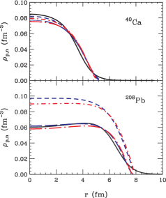
FIG. 1.: Nucleon density profiles from solving the TF equations for MFs corresponding to $K=210$ MeV, together with the empirical charge density profiles for ⁴⁰Ca and ²⁰⁸Pb. The solid lines represent the empirical profiles from Ref. [25]. The long- and short-dashed lines represent the proton and neutron profiles, respectively, for the momentum-independent field. The long- and short-dash-dotted lines represent the proton and neutron profiles, respectively, for the momentum-dependent field in Table I that yields $m^{*}=0.70\,m$.

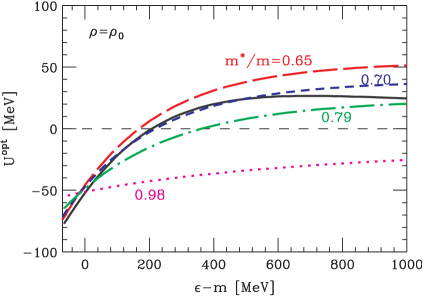
FIG. 2.: Real part of the optical potential in normal nuclear matter, as a function of nucleon energy. The solid line represents a fit [26] to the information from structure and nucleon scattering [28, 3]. The dashed lines represent the potential for different MF parametrizations in Table I for $K=210$ MeV. The numbers in the figure indicate the ratio $m^{*}/m$. For $m^{*}/m=0.65$ only the first set from the table is represented. The dotted line represents the potential for the MF without momentum dependence in its nonrelativistic reduction, corresponding to $K=210$ MeV.

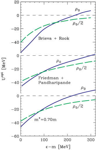
FIG. 3.: Optical potential in nuclear matter, as a function of nucleon energy, obtained in Brueckner-Hartee-Fock [29] (top) and variational [30] calculations and in our $K=210$ MeV and $m^{*}/m=0.70$ parametrization. Solid and dashed lines show the potential at $\rho_{0}$ and $\rho_{0}/2$, respectively.

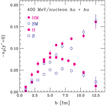
FIG. 4.: Negative of the ellipticity coefficient at midrapidity, as a function of the impact parameter, from simulations of Au + Au collisions at 400 MeV/nucleon. The squares and circles represent, respectively, the results for MF without and with momentum dependence ($m^{*}/m=0.65$, of Ref. [15]). The filled symbols are for the incompressibility $K=380$ MeV and the open symbols are for $K=210$ MeV.

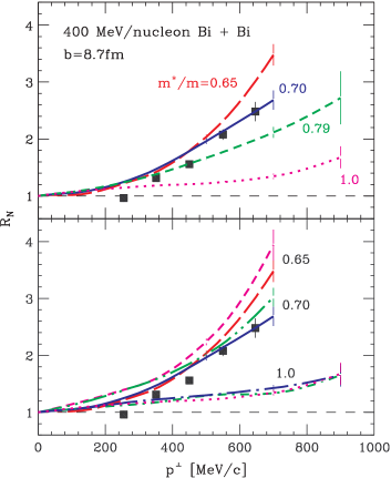
FIG. 5.: Measured [40] (filled squares) and calculated (lines) ratios of out-of-plane to in-plane proton yields at midrapidity (0.35 $<y/y_{beam}<$ 0.65), $R_{N}$ = $(N(90^{\circ})$ + $N(-90^{\circ}))/(N(0^{\circ})$ + $N(180^{\circ}))$, as a function of transverse momentum, in 400 MeV/nucleon ²⁰⁹Bi + ²⁰⁹Bi collisions at $b=8.7$ fm. Both the measured and the calculated ratios are computed from the lowest Fourier coefficients of the proton distribution, $R_{N}=(1-v_{2})/(1+v_{2})$. The lines in the top panel represent results of the simulations done using in-medium cross sections and those MFs for which the optical potentials are shown in Fig. 2. The numbers in the panels indicate the magnitude of effective mass for the MFs. The bottom panel shows the sensitivity of the results to the variation of cross sections and of incompressibility. The long-dashed, solid, and dotted lines repeat respective results from the top panel obtained with in-medium cross sections and $K=210$ MeV. The long-dash-dotted and short-dash-dotted lines represent additional results obtained, respectively, using the momentum-independent MF corresponding to $K=380$ MeV and using no MF at all. The short-dashed and long-dash-double-dotted lines represent the additional results obtained for free cross-sections and MFs corresponding to $m^{*}/m=0.65$ and to $m^{*}/m=0.70$, respectively.

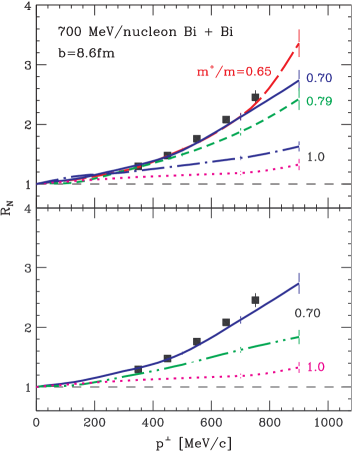
FIG. 6.: Measured [40] (filled squares) and calculated (lines) ratios of out-of-plane to in-plane proton yields at midrapidity (0.35 $<y/y_{beam}<$ 0.65), as a function of transverse momentum, in 700 MeV/nucleon ²⁰⁹Bi + ²⁰⁹Bi collisions at $b=8.6$ fm. Both the measured and the calculated ratios are computed from the lowest Fourier coefficients of the proton distribution, $R_{N}=(1-v_{2})/(1+v_{2})$. The numbers in the figure indicate the values of the effective mass in the ground state at Fermi momentum for the calculations. The value of incompressibility is $K=380$ MeV for the calculation represented by the long-dash-dotted line in the top panel and $K=210$ MeV for other calculations in that panel. The solid and dotted lines in the bottom panel repeat the results from the top panel. The long-dash-double-dotted line in the bottom panel represents the results of a calculation where the momentum dependence of the MF at $\rho>\rho_{0}$ is made to follow the dependence at $\rho=\rho_{0}$, cf. the text.

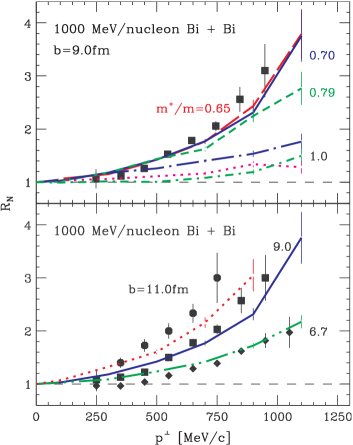
FIG. 7.: Measured [40] (filled symbols) and calculated (lines) ratios of out-of-plane to in-plane proton yields at midrapidity (0.35 $<y/y_{beam}<$ 0.65), as a function of transverse momentum, in 1000 MeV/nucleon ²⁰⁹Bi + ²⁰⁹Bi collisions. Both the measured and calculated ratios are computed from the lowest Fourier coefficients of the proton distribution, $R_{N}=(1-v_{2})/(1+v_{2})$. The top panel shows the ratios for collisions at $b=9.0$ fm. The long-dashed, solid, and short-dashed lines represent calculations for the momentum-dependent MFs corresponding to $K=210$ MeV and $m^{*}/m=$ 0.65 (first of the sets in Table I), $m^{*}/m=0.70$, and 0.79, respectively. The long-dash-dotted, dotted, and short-dash-dotted lines represent two calculations with momentum-independent MFs corresponding to $K=380$ MeV, and $K=210~{}MeV$, and one with no MF at all, respectively. The numbers in the panel indicate values of the effective mass for the calculations. The bottom panel shows ratios for collisions at impact parameters $b=11.0$ fm (filled circles and dotted line), 9.0 fm (filled squares and solid line), and 6.7 fm (filled diamonds and long-dash-double-dot line). The calculations for the bottom panel were carried out using the MF characterized by $K=210$ MeV and $m^{*}/m=0.70$. The numbers in the bottom panel indicate the values of impact parameter.

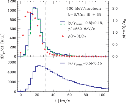
FIG. 8.: Time dependence of baryon density (stars in the top panel) at the system center and time dependence of midrapidity emission-rate for high-momentum (lines in the top panel) and all (bottom panel) protons, in Bi + Bi simulations at 400 MeV/nucleon and $b=8.7$ fm. All results were obtained with the $K=210$ MeV $m^{*}/m=0.70$ MF, except for the emission rate for the high-momentum protons represented by the thick dashed line, obtained with the $K=380$ MeV momentum-independent MF. The thin vertical dashed line at $t=30$ fm/c is drawn to guide the eye.

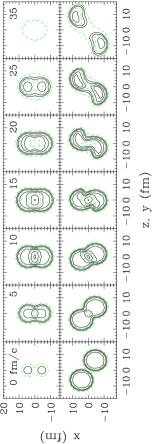
FIG. 9.: Contour plots of baryon density in the 400 MeV/nucleon Bi + Bi reaction at $b=8.7$ fm in the reaction plane (bottom panels) and in the plane through the system center othogonal to the beam axis (top panels). The simulation was done using the MF characterized by $K=210$ MeV and $m^{*}/m=0.70$. The density contours are shown at intervals of 0.2 in $\rho/\rho_{0}$, starting from $\rho/\rho_{0}=0.1$. Every third contour, i.e. for $\rho/\rho_{0}=0.1$, 0.7, and 1.3, is represented by a dashed line. The remaining contours are represented by solid lines. Numbers in the figure indicate time in fm/c.

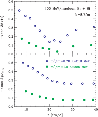
FIG. 10.: Time dependence of $-v_{2}$ for protons at $p^{\perp}>550$ MeV/c from 400 MeV/nucleon Bi + Bi simulations employing either the $m^{*}/m=0.70$ $K=210$ MeV MF (open circles) or the $K=380$ MeV momentum-independent MF (filled circles). The top panel shows the average values for protons emitted in the vicinity of a given time, while the bottom panel shows the value for all protons emitted up to that time.

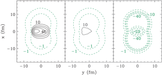
FIG. 11.: Contour plots of the optical potential field, Eq. (27), in the 400 MeV/nucleon $b=8.7$ fm Bi + Bi reaction, within the plane through the system center perpendicular to the beam axis, at $t=10$ fm/c, for nucleons with $p^{\perp}=600$ MeV/c directed to the right of the plot. The three panels, from left to right of the plot respectively, show results for three different MFs: the standard MF characterized by $m^{*}/m=0.70$ and $K=210$ MeV, the same MF with momentum-dependence frozen above $\rho_{0}$, and the momentum-independent MF characterized by $K=310$ MeV. The Coulomb and isospin contributions to the potential are ignored in every case. The contours are indicated for the potential value of $-1$ MeV and for positive and negative multiples of 10 MeV. The contours for the positive and negative values are represented, respectively, by the solid and dashed lines. The $-1$, $\pm 10$, and $\pm 40$ MeV contours are labeled.

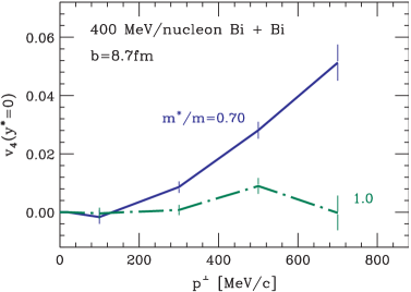
FIG. 12.: Proton Fourier coefficient $v_{4}=\langle\cos{4\phi}\rangle$ as a function of transverse momentum at midrapidity in the Bi + Bi system at 400 MeV/nucleon and $b=8.7$ fm, from simulations utilizing the $m^{*}/m=0.70$ $K=210$ MeV MF (solid line) and the $K=380$ MeV momentum-independent MF (dash-dotted line). Numbers in the figure indicate the effective mass.

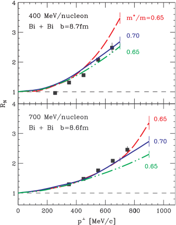
FIG. 13.: Measured [40] (filled squares) and calculated (lines) ratios of out-of-plane to in-plane proton yields at midrapidity (0.35 $<y/y_{beam}<$ 0.65), as a function of transverse momentum, in ²⁰⁹Bi + ²⁰⁹Bi collisions at $b=8.6$ fm and energies of 400 (top panel) and 700 MeV/nucleon (bottom panel). Both the measured and calculated ratios are computed from the lowest Fourier coefficients of the proton distribution, $R_{N}=(1-v_{2})/(1+v_{2})$. The calculations were carried out using in-medium cross sections and MFs characterized by the incompressibility of $K=210$ MeV. The numbers in the figure indicate the values of the effective mass for the MFs; the solid lines represent results obtained using the MF in Table I characterized by $m^{*}/m=0.70$ and the long-dashed and long-dash-double-dotted lines represent results obtained the first and second $m^{*}/m=0.65$ MF in the table, respectively.

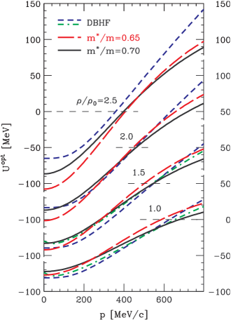
FIG. 14.: Optical potential in nuclear matter as a function of nucleon momentum, at different densities, from the DBHF calculations with Bonn-A interaction [43] and in our parametrizations. The short-dashed and short-dash-dotted lines represent the DBHF potentials obtained assuming, respectively, momentum-independent vector and scalar MFs [7, 43] and parametrized momentum-dependent MFs [9]. The solid and long-dashed lines represent the optical potentials for our $m^{*}/m=0.70$ and first $m^{*}/m=0.65$ $K=210$ MeV MF parametrizations, respectively. The numbers in the figure indicate the values of density in units of the normal density $\rho_{0}=0.16$ fm^-3. The thin horizontal dashed lines indicate the zero value for the potential.

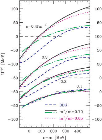
FIG. 15.: Optical potential in nuclear matter as a function of nucleon energy, at different densities, from the BBG calculations with Paris interaction [6, 8] and in our parametrizations. The short-dashed, dotted, and solid lines represent the BBG potential and the potential for our second $m^{*}/m=0.65$ and $m^{*}/m=0.70$ $K=210$ MeV parametrizations, respectively. The long-dash-double-dotted lines represent the potential for our $m^{*}/m=0.70$ parametrization with the momentum dependence frozen above $\rho_{0}=0.16$ fm^-3. The numbers in the figure indicate the values of density in units of fm^-3. The thin horizontal dashed lines indicate the zero value for the potential.

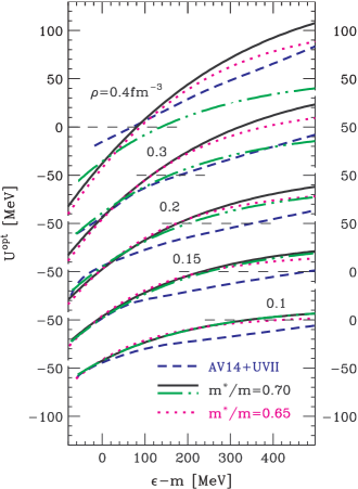
FIG. 16.: Optical potential in nuclear matter as a function of nucleon energy, at different densities, from the variational calculations with AV14 + UVII interactions [5] and in our parametrizations. The short-dashed, dotted, and solid lines represent the AV14 + UVII potential and the potential for our second $m^{*}/m=0.65$ and $m^{*}/m=0.70$ $K=210$ MeV parametrizations, respectively. The long-dash-double-dotted lines represent the potential for our $m^{*}/m=0.70$ parametrization with the momentum dependence frozen above $\rho_{0}=0.16$ fm^-3. The numbers in the figure indicate the values of density in units of fm^-3. The thin horizontal dashed lines indicate the zero value for the potential.

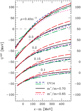
FIG. 17.: Optical potential in nuclear matter as a function of nucleon energy, at different densities, from the variational calculations with UV14 + TNI and UV14 + UVII interactions [5] and in our parametrizations. The short-dashed and long-dash-dotted lines represent the UV14 + TNI and UV14 + UVII potentials, respectively. The solid, long-dashed, and dotted lines represent, respectively, the potentials for our $m^{*}/m=0.70$, and first and second $m^{*}/m=0.65$ $K=210$ MeV MF parametrizations. The numbers in the figure indicate the values of density in units of fm^-3. The thin horizontal dashed lines indicate the zero value for the potential.