Ground state correlations and mean-field in 16O:
Part II
Abstract
We continue the investigations of the 16O ground state using the coupled-cluster expansion [] method with realistic nuclear interaction. In this stage of the project, we take into account the three nucleon interaction, and examine in some detail the definition of the internal Hamiltonian, thus trying to correct for the center-of-mass motion. We show that this may result in a better separation of the internal and center-of-mass degrees of freedom in the many-body nuclear wave function. The resulting ground state wave function is used to calculate the “theoretical” charge form factor and charge density. Using the “theoretical” charge density, we generate the charge form factor in the DWBA picture, which is then compared with the available experimental data. The longitudinal response function in inclusive electron scattering for 16O is also computed.
pacs:
21.60.Gx,25.30.-c,21.10.Ft,27.20.+n2
I Introduction
The coupled-cluster expansion, also called the method, was developed about 40 years ago by Coester [1]. It was then applied to finite nuclei quite successfully by Kümmel and the Bochum group [2] using a representation of the wave function in coordinate space together with common interactions of that time. While the method in general is viewed as essentially exact, approximations are introduced stemming from truncations in the coupled cluster equations, as well as truncations in the model space. The results for the binding energy were well above the Coester-line and were taken as evidence for the presence of three-nucleon and higher order interactions.
While few further developments took place since that time, the ongoing expansion in computer power as well as the availability of more sophisticated nucleon-nucleon interactions suggests that one should go back to these precise methods. During the past several years we have reexamined the coupled cluster approach and applied it to the spherical nucleus 16O using the Argonne 18 potential [3]. We combine the mean field approach together with the coupled cluster expansion in a harmonic oscillator basis of 50 (which constitutes our truncated Hilbert space) and going up to the level of 44 clusters.
Further, we have expanded the formulation to include the Urbana IX three-nucleon interaction. The results are in reasonable agreement with the experiment and make the subject of the present paper. These results obtained using the coupled cluster expansion should be directly comparable with those obtained using the Variational Monte Carlo (VMC) [4] or the Green’s Function Monte Carlo (GFMC) methods, using the same interaction. Especially the GFMC method with the Argonne 18 potential and the Urbana IX three-nucleon interaction has proved quite accurate in nuclei with [5], even though a certain uncertainty in the three-nucleon interaction model is responsible for a systematic lack of binding in the heavier systems. These difficulties will be addressed however in the future, by considering more sophisticated three-body interaction models.
In section II we briefly review the coupled-cluster approach as outlined in [3] when the Hamiltonian includes only the two-body interaction. We continue this discussion in section III with comments pertaining to the inclusion of the center-of-mass Hamiltonian, which is supposed to constrain the center-of-mass degrees of motion in the ground state wave function. In section IV we outline the changes necessary in order to include the three-nucleon interaction via a density-dependent approximation. In section V we show various observables calculated in the ground state for 16O. Finally, in section VI we present our conclusions and a brief outlook.
II Coupled-cluster method: a review
For a spherically symmetric nuclear system, consisting of both protons and neutrons, the total Hamiltonian is given as the sum of a nonrelativistic one-body kinetic energy, a two-nucleon potential and a three-nucleon potential
| (1) |
Since our calculation is carried out in configuration space, we need the nuclear interaction projected out in an operator format allowing for calculation of two- and three-body matrix elements. We chose to use the operator format of the Argonne and Urbana family potentials. The Argonne 18 model [6] is one of a new class of potentials that accurately fit both and scattering data up to 350 MeV with a /datum near one. The Urbana IX potential [7] includes a long-range two-pion exchange and a short-range phenomenological component. The strength constant of the short-range component is adjusted to reproduce the binding energy of the three-nucleon system.
In configuration space, the many-body correlated ground state, , of is written as a linear combination of all possible particle configurations, which are defined in terms of the nn creation operators, ( = , = , = ) acting on the reference state, . Since the nucleon system obeys the Fermi statistics, the natural choice for the vacuum is a single-particle Slater determinant. In the coupled-cluster expansion, we have
where is the cluster correlation operator, defined in terms of its ph-creation operators expansion as
In order to determine the amplitudes we solve a set of non-linear equations, which may be obtained using a variational principle [3]:
| (2) |
The coefficients of the operators carry the physical significance of nuclear correlations.
In reference [3] we have outlined our approach to solving the coupled-cluster equations (2). We first introduce a mean-field Hamiltonian in terms of the one-body kinetic energy operator and a mean-field potential. The mean-field is partially constrained by the assumption that , or the maximum overlap basis. The set of single-particle energies and wave functions which determine the configuration space is determined by diagonalizing the mean-field Hamiltonian.
The mean-field component calculation is carried out together with the calculation of the 22 correlations in a self-consistent manner. Even though the 33 and 44 correlations are not calculated explicitly, the 22 correlations are implicitly corrected for the presence of higher-order correlations, consistently with our truncation scheme. In this respect we replace the traditional truncation in [2] by a truncation in , where is the nn excitation energy. The results presented here are obtained by keeping only terms up to second order in .
III Center-of-mass Hamiltonian
The correlated ground-state is a function of sets of coordinates . Consequently, the ground state wave function is not translationally invariant. As a result, it is common practice [3] to attempt solving the Schrödinger equation for the ground state of the internal Hamiltonian
instead of the Hamiltonian (1). The internal Hamiltonian is entirely written in the center-of-mass frame by removing the center-of-mass kinetic energy, , with being the nucleon mass. Both the two- and three-nucleon interactions are given in terms of the relative distances between nucleons, so in this respect no corrections are needed.
However, this does not prevent the contamination of the correlated ground-state by the center-of-mass motion. Especially since we are interested in the calculation of the excited states spectrum, this contamination will result in spurious excitations of the center-of-mass. Moreover, the calculation of observables to be compared with experimental data which are taken in the center-of-mass frame, requires the evaluation of a many-body expansion as explained in [8]. This in turn relies on the assumption that we can neglect the correlations between the internal and center-of-mass degrees of freedom at the level of the correlated ground-state . In order to ensure such a separation, a supplemental center-of-mass Hamiltonian is added
The center-of-mass Hamiltonian has the role of constraining the center-of-mass component of the ground state wave function [9]. Then, we have to identify a domain of values for the parameters and such that the binding energy
is insensitive to the choice of these parameters.
IV Three-nucleon interaction corrections
We will present here the corrections necessary to take into account the three-nucleon interaction as part of the general nuclear interaction. As discussed before we consider the three-nucleon interaction as the sum of two components: a long-range two-pion exchange and a short-range phenomenological component. The calculation of the three-nucleon interaction has been presented elsewhere [10].
Given the form (1) of the Hamiltonian, we write the operator in second quantization as
| (3) |
Here, the matrix elements are given as integrals involving the single particle states (including spins)
| (4) | |||
| (5) |
In addition to being symmetric with respect to the interchange of the particles labelled and
| (6) |
the integrals (5) also satisfy the symmetry
| (7) |
The last property is a consequence of the cyclic sums involved in the definition of the interaction, which make the interaction invariant with respect to the labelling of the particles.
In previous applications the approximation has been made that such an interaction can be represented by a density dependent two-body interaction. While such a substitution is the easiest modification, it has been stated that this is insufficient [7]. However, the rigorous inclusion of the three-nucleon interaction in configuration space using the coupled-cluster method is seriously hampered by our present computing capabilities and the necessary size of the configuration space. Ideally, we would like to calculate all integrals of the form (5) without any artificial restrictions. In practice though, we must limit ourselves to calculating matrix elements of the form
| (8) |
where and couple to spin 0 only. We are then faced with a compromise: Since matrix elements of the form (8) are all we need in order to calculate exactly the first- and second-order () contributions to the mean-field and binding energy, the leading orders in our expansion are treated rigorously correct. Then we make a reduction of the three-nucleon interaction to an effective two-body interaction, and use this effective interaction when dealing with higher-order corrections (3). This is achieved by defining the effective two-body interaction as
| (9) |
where we define the matrix element to be equal to
| (10) | |||
| (11) | |||
| (12) |
The definition (12) has been inspired by the form of second order () contributions to the binding-energy and has the additional advantage of being fully anti-symmetric, so that all procedures developed when dealing with the nucleon-nucleon interaction [11], can be naturally extended to handle the three-nucleon interaction. Note that the first two terms in Eq. (12) are equivalent to the standard density-dependent reduction of the three-body force.
We shall now detail the changes necessary to take into account the effects of the three-nucleon interaction in the calculation of the binding-energy and mean field using the coupled-cluster formalism.
A Binding Energy Corrections.
We are only interested in the total binding energy when the wave function satisfies the Hartree-Fock conditions. Thus, it suffices to compute
| (13) |
The first order corrections to the binding energy are due to the expectation value of the three-nucleon interaction in the uncorrelated ground state. We have
| (16) | |||||
Using the symmetries (6, 7), the last equation becomes
| (18) | |||||
We notice that only the first two terms in Eq. (LABEL:eq:vtni_av) have the form (8). However, in this particular case, it is a simple endeavor to calculate the missing third matrix element. We find that the magnitude of this term is small compared to the sum of the terms (8).
Second order contributions are calculated exactly as
| (20) |
At the present time, the third order corrections have not been evaluated. Their magnitude is expected to be small, and their inclusion is definitely next-order in terms of the present expansion.
B Mean Field Corrections.
In our approach to the coupled cluster formalism, the single particle orbits are eigenfunctions of an mean-field Hamiltonian, defined as the sum of a one-body kinetic energy term and a one-body mean-field potential. The later is not unique, and in the maximum overlap hypothesis , the mean-field is defined as
| (21) |
Correspondingly, the contributions due to the three-nucleon interaction can be written as the sum of three terms
| (22) | |||
| (23) |
In leading order, the three-nucleon interaction correction of the mean-field is given as
| (26) | |||||
Again, using the symmetries (6, 7), Eq. (LABEL:eq:vtni_mf_a1) becomes
| (29) | |||||
The second- and third-order contributions in Eq. (23) look very similar when one uses the proposed reduction of the three-body force, Eq. (12), for the account of the 33 correlations. Then, by making use of the full anti-symmetry of and we can show that the required corrections can be written as
| (31) | |||
| (32) | |||
| (33) |
To maintain the symmetry we have also added similar terms to the - and -terms of the single particle Hamiltonian.
V Observables
The results we report here are carried out in a configuration space. In general, the expectation value of any arbitrary operator in the correlated ground-state is obtained as
where similarly to the cluster correlation operator , the new operator is expanded out in terms of ph-creation operators
The amplitudes are calculated iteratively in terms of the amplitudes [3].
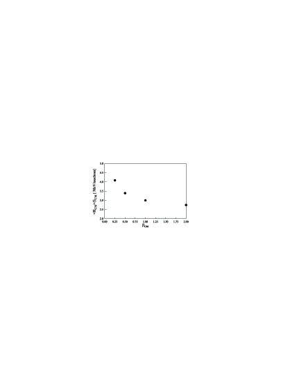
The resulting binding energy and charge radii for the Argonne 18 with/without the Urbana IX potential, are shown in Table I. Note that the charge radii correspond to the “theoretical” charge density as explained below. The calculation is shown to be stable with respect to the two cut-off parameters, and , which control the size of the configuration space as . Figure 3 shows the binding energy for 16O calculated using the 18 and Urbana IX interactions, as a function of the (, ) cut-off pair, and show the calculation to be reasonably converged for and , same as the 18 based calculation of [3].
A Charge Form Factor
The charge form factor is calculated as the sum of a one- and two-body operator. The one-body component is evaluated in the nonrelativistic one-body Born-approximation picture, where the charge form factor is given as
Here is the nucleon form factor, which takes into account the finite size of the nucleon . In our calculation we use the Iachello-Jackson-Lande [12] nucleon-form factors. Note however that at the rather small values of involved in the present discussion, fm-1, the differences between the various models of the nucleon form factor are expected to be small [13].
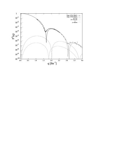
As seen from previous calculations [4], the main contributions from the two-body charge density not related to center-of-mass corrections is expected to come from the the - and -exchange “seagull” diagrams. These are taken into account as referred in the model-independent part of the “Helsinki meson-exchange model” [13]. In this model the pion and -meson propagators are replaced by the Fourier transforms of the isospin dependent spin-spin and tensor components of the 18 interaction, in order to ensure that the exchange current operator does satisfy the continuity equation together with the interaction model. As seen from Fig. 4, the contributions of - and -exchange give a measurable correction for fm-1. The order of magnitude of the - and -exchange contributions compares well with the calculation of [4] for 16O using the Argonne 14 potential and Urbana VII three-nucleon interaction.
Since the correlated ground state wave function is not translationally invariant, extra care needs to be taken in order to account for the effect of the center-of-mass motion on the expectation value of the operator in the ground state. Center-of-mass corrections have been discussed in [8], and rely on the assumption that the motion of the intrinsic coordinates , and the center-of-mass are not correlated, and that our correlated ground-state provides indeed a good description of the internal structure of the nucleus.
Figure 4 depicts the center-of-mass corrected charge form factor both in the impulse approximation and including the meson-exchange two-body component, together with the experimental results for fm-1 [14]. These various approximations of the theoretical charge form factor correspond to the 18+UIX+ interaction in Table I.
Figure 5 shows the corresponding charge density together with the “experimental” charge density as derived in [14]. This calculation simply represents the result of Fourier transforming the charge form-factor presented in Fig. 4. However, in doing so we use predictions for a momentum transfer greater than 4 fm-1, where the present calculation is not expected to offer reliable predictions. This results in uncertainties of the charge density distribution at short distances .
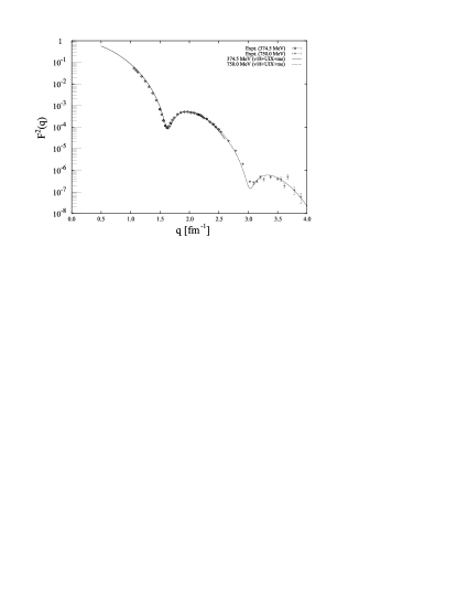
Also, the distortion effect related to the interaction of the electron probe with the nuclear Coulomb field has not yet been accounted for. Thus, we use the Distorted Wave Born Approximation (DWBA) to calculated a new charge form factor [15], which is depicted in Fig. 6. Note this calculation is now sensitive to the energy of the incident electron as shown in Fig. 6. This time the agreement is quite impressive, and the calculation of the corresponding charge density will give a result considerably closer to the “experimental” one. As a result of this exercise, we conclude that it is better to compare the results of the distorted charge form factor calculation with the experimental charge form factor over the domain of momentum transfer covered by the experiment. In any event the charge form factor represents the primary result of the experiment, and comparing form factors is thus more reliable than comparing model-dependent charge densities.
Note that the persistent discrepancy at large may be a signature of the break down of the nonrelativistic approach to calculating the charge form factor. However, due to the various other approximations made so far, a calculation based on the relativistic description of the one-body charge form factor [16] may be too expensive at this time.
B Coulomb Sum Rule
The Coulomb sum rule, , represents the total integrated strength of the longitudinal response function measured in inclusive electron scattering. The Coulomb sum rule is related to the Fourier transform of the proton-proton distribution function in the nuclear ground state [17]. As such, this quantity is sensitive to the short-range correlations induced by the repulsive core of the interaction. In the nonrelativistic limit we have [18]
| (34) | |||||
| (35) |
where is the nuclear charge operator
| (36) |
In Eq. (35), the longitudinal-longitudinal distribution function is given in terms of the proton-proton two-body density as
| (37) |
We have outlined recently [3] the calculation of the proton-proton two-body density in the coupled-cluster framework, as the expectation value
| (38) | |||
| (39) |
with the normalization
| (40) |
Figure 7 depicts the results of the present calculation for 16O. Agai, the theoretical calculation corresponds to the 18+UIX+ interaction in Table I. Since no experimental data are available for 16O we compare these results with the 12C experimental data of [19], where an estimate [20] for contributions from large has been added. Preliminary theoretical results for 12C obtained using the coupled-cluster method have been recently reported in [21] and shown to be close to the 16O result. The large error bars on the experimental data are largely due to systematic uncertainties associated with tail contribution [22].
VI Conclusions and Outlook
The goal of our effort is to make a contribution to the ongoing effort of building realistic models of nuclear structure that explicitly account for realistic correlations. In a first stage we focus our attention on obtaining a realistic description for the ground state of a doubly-magic nucleus using the coupled-cluster method. In this sense, the present calculation represents the most detailed calculation available today, using the coupled-cluster method for a nuclear system with . We base our calculation on what is considered the best realistic description of the two- and three-body interactions available today [5].
At this stage we have proved conclusively that it is possible to choose a large enough configuration space to handle the relatively hard-core of the nucleon-nucleon interaction. We believe that we have also identified the dominant contributions of the three body interaction, and we have introduced an effective two-body interaction, accordingly.
An interesting conclusion from the charge form factor calculation has to do with the importance of the distortion effect due to the interaction between the electron and the Coulomb field of the nucleus. In this context we have shown that it is desirable to compare the distorted charge form factor with the experimental one, and to de-emphasize the comparisons regarding the nuclear charge density, which is not very surprising as the charge form factor represents the primary result of the experiment.
In this paper we have confined ourselves to presenting a purely nonrelativistic description of the charge form factor in 16O. In the future it will be interesting to get a better understanding of the importance of relativistic effects on the charge form factor calculation. In this sense we plan to redo this calculation using the relativistic description of the one-body charge form factor of [16], together with a consistent relativistic derivation of the two-body meson-exchange density [23].
With the calculation of the 16O ground state completed we intend to extend our formulation to address the calculation of discrete excited states as well as neighboring odd-even nuclei. This is a necessary step in the quest of modeling the (e,e’N) reaction, where the final state has the asymptotic form of a distorted wave times a discrete state of the (A-1) nucleus. However, this is not a solution to the Hamiltonian close to the origin, and thus the wave function needs to be modified in the region of the origin.
acknowledgements
This work was supported in part by the U.S. Department of Energy (DE-FG02-87ER-40371). The work of B.M. was also supported in part by the U.S. Department of Energy under contract number DE-FG05-87ER40361 (Joint Institute for Heavy Ion Research), and DE-AC05-96OR22464 with Lockheed Martin Energy Research Corp. (Oak Ridge National Laboratory). Special thanks go to our colleagues F. W. Hersman, M. Holtrop, and their student T. Streeter, J. Kirkpatrick, and D. Protopopescu from the University of New Hampshire for setting up the computer farm of 100 Intel Celeron processors at 500 MHz. This allowed us to run several test cases simultaneously. The authors gratefully acknowledge useful conversations with John Dawson and David Dean.
REFERENCES
- [1] F. Coester, Nucl. Phys. 7, 421 (1958); F. Coester and H. Kümmel, Nucl. Phys. 17, 477 (1960).
- [2] H. Kümmel, K. H. Lührmann, and J. G. Zabolitzky, Phys. Reports 36, 1 (1978).
- [3] J.H. Heisenberg and B. Mihaila, Phys. Rev. C 59, 1440 (1999), nucl-th/9802029.
- [4] S. C. Pieper, R. B. Wiringa, and V. R. Pandharipande, Phys. Rev. C 46, 1747 (1992).
- [5] B. S. Pudliner, V. R. Pandharipande, J. Carlson, S. C. Pieper, and R. B. Wiringa, Phys. Rev. C 56, 1720 (1997), nucl-th/9705009; B. S. Pudliner, V. R. Pandharipande, J. Carlson, and R. B. Wiringa, Phys. Rev. Lett. 74, 4396 (1995).
- [6] R. B. Wiringa, V. G. Stoks, and R. Schiavilla, Phys. Rev. C 51, 38 (1995).
- [7] J. Carlson, V.R. Pandharipande, and R. B. Wiringa, Nucl. Phys. A 401, 59 (1983).
- [8] B. Mihaila and J. H. Heisenberg, Phys. Rev. C 60, 054303 (1999), nucl-th/9802029.
- [9] P. Navratil and B. R. Barrett, Phys. Rev. C 57, 3119 (1998); D. J. Dean et al., Phys. Rev. C 59, 2474 (1999).
- [10] B. Mihaila and J. H. Heisenberg, nucl-th/9912024 (1999).
- [11] B. Mihaila and J. H. Heisenberg, nucl-th/9802012 (1998).
- [12] F. Iachello, A. D. Jackson, and A. Lande, Phys. Lett. 43B, 191 (1973).
- [13] R. Schiavilla, V. R. Pandharipande, and O. Riska, Phys. Rev. C 41, 309 (1990).
- [14] I. Sick and J.S. McCarthy, Nucl. Phys. A 150, 631 (1970).
- [15] D. R. Yennie, D. G. Ravenhall, and R. N. Wilson, Phys. Rev. 95, 500 (1954).
- [16] S. Jeschonnek and T. W. Donnelly, Phys. Rev. C 57, 2438 (1998).
- [17] K. M. McVoy and L. Van Hove, Phys. Rev. 125, 1034 (1962).
- [18] J. Carlson and R. Schiavilla, Rev. Mod. Phys. 70, 743 (1998).
- [19] P. Barreau et al., Nucl. Phys. A402, 515 (1983).
- [20] R. Schiavilla, A. Fabrocini, and V. R. Pandharipande, Nucl. Phys. A473, 290 (1987).
- [21] B. Mihaila and J. H. Heisenberg, Phys. Rev. Lett. (in press).
- [22] R. Schiavilla, R. B. Wiringa, and J. Carlson, Phys. Rev. Lett. 70, 3856 (1993).
- [23] J. E. Amaro, M. B. Barbaro, J. A. Caballero, T. W. Donnelly and A. Molinari, Nucl. Phys. A643, 349 (1998)
| Interaction | B.E. | r.m.s |
|---|---|---|
| [MeV/nucleon] | [fm | |
| 18 | -5.9 | 2.85 |
| 18 + UIX | -7.7 | 2.74 |
| 18 + UIX + | -8.0 | 2.62 |
| expt. | 8.00 | 2.73 0.025 |