[

Fine Structure in the Decay of Deformed Proton Emitters: Non-adiabatic Approach

Abstract

The coupled-channel Schrödinger equation with outgoing wave boundary conditions is employed to study the fine structure seen in the proton decay of deformed even-$N$, odd-$Z$ rare earth nuclei ¹³¹Eu and ¹⁴¹Ho. Experimental lifetimes and proton-decay branching ratios are reproduced. The comparison with the standard adiabatic theory is made.

]

Proton radioactivity has proven to be a very powerful tool to observe neutron-deficient nuclei and study their structure. Theoretically, proton radioactivity is an excellent example of a simple three-dimensional quantum-mechanical tunneling problem. Indeed, in first order, it only involves a single proton moving through the Coulomb barrier of the daughter nucleus. In reality, the process of proton emission is more complicated since the perfect separation of the nuclear many-body wave function into that of the proton and the daughter cannot be made, and – in addition – the decay is greatly influenced by nuclear structure effects such as configuration mixing. In spite of this, the first-order one-body picture works surprisingly well; it enables us to determine the angular momentum content of a resonance and the associated spectroscopic factor in many cases [1, 2]. Experimental and theoretical investigations of proton emitters are opening up a wealth of exciting physics associated with the coupling between bound states and extremely narrow resonances in the region of very low single-particle level density. One particular example of such a coupling, due to the Coriolis interaction, is discussed in this work.

The last two years have seen an explosive number of exciting discoveries in this field, including new ground-state proton emitters and proton-decaying excited states [3, 4, 5, 6], and the first evidence of fine structure in proton decay [7]. The main focus of recent investigations has been on well-deformed systems which exhibit collective rotational motion; consequently, they are splendid laboratories for the interplay between proton emission and angular momentum.

From a theoretical viewpoint, the understanding of proton emitters is a test of how well one can describe very narrow resonances. For spherical nuclei, there are many available theoretical methods, most of which give very similar and accurate results [8]. There have been several theoretical attempts to describe deformed proton emitters. These approaches can be divided into three groups. The first family of calculations [3, 7, 9] is based on the reaction-theoretical framework of Kadmenskiĭ and collaborators [10]. The second group is based on the theory of Gamow (resonant) states [5, 11, 12, 13]. Finally, calculations based on the time-dependent Schrödinger equation have recently become available [14]. All of these papers assume a strong coupling approximation. That is, the daughter nucleus is considered to be a perfect rotor with an infinitely large moment of inertia. Consequently, all the members of the ground-state rotational band are degenerate and the Coriolis coupling is ignored. Our work is the first attempt to go beyond these simplified assumptions in the description of proton radioactivity.

Our technique is based on the theory of Gamow states. More precisely, we solve the coupled-channel Schrödinger equation describing the motion of the proton in the deformed average potential of a core (a daughter nucleus). It is assumed that the wave function of the proton is regular at the origin and asymptotes to a purely outgoing Coulomb wave. These boundary conditions result in complex-energy eigenstates [15]. For resonant states, the real part of the energy, $E_{0}={\rm Re}(E)$, can be interpreted as the resonance’s energy, while the imaginary part is proportional to the resonance’s width, $\Gamma=-2{\rm Im}\,(E)$.

Let us consider the Hamiltonian of the daughter-plus-proton system

$$H=H_{d}+H_{p}+V,$$ (1)

where $H_{\rm d}$ is the Hamiltonian of the daughter nucleus, $H_{p}$ is the proton Hamiltonian, and $V$ represents the proton-daughter interaction. The total wave function, $\Psi$, of the parent nucleus can be written in the weak-coupling form

$$\Psi_{JM}=r^{-1}\sum_{J_{d}l_{p}j_{p}}u_{J_{d}l_{p}j_{p}}^{J}(r)\left({\cal Y}_{l_{p}j_{p}}\otimes\Phi_{J_{d}}\right)_{JM}.$$ (2)

In (2) $u_{\alpha}^{J}$ ($\alpha$$\equiv$$(J_{d}l_{p}j_{p})$ labels the channel quantum numbers) is the cluster radial function representing the relative radial motion of the proton and the daughter nucleus, ${\cal Y}_{j_{p}l_{p}m_{p}}$ is the orbital-spin wave function of the proton, and $\Phi_{J_{d}M_{d}}$ is the wave function of the daughter nucleus. By definition, one has

$$H_{d}\Phi_{J_{d}M_{d}}=E_{J_{d}}\Phi_{J_{d}M_{d}}.$$ (3)

In practice, the energies $E_{J_{d}}$ are taken from experiment or, if the data are not available, they are modeled theoretically. Inserting (2) into the Schrödinger equation and integrating over all coordinates except the radial variable $r$, one obtains the set of coupled equations for the cluster functions [9, 16]:

$$\left[-\frac{\hbar^{2}}{2\mu}\frac{d^{2}}{dr^{2}}\right. + \left.\frac{\hbar^{2}l_{p}(l_{p}+1)}{2\mu r^{2}}+V_{\alpha}(r)-Q_{J_{d}}\right]u_{\alpha}^{J}(r)$$ (4)

$$+ \sum_{\alpha^{\prime}}V_{\alpha,\alpha^{\prime}}^{J}(r)u_{\alpha^{\prime}}^{J}(r)=0.$$ (5)

In Eq. (4) $V_{\alpha}$ represents the average spherical potential of the proton in the state $\alpha$, $V_{\alpha,\alpha^{\prime}}^{J}$ is the off-diagonal coupling term, and $Q_{J_{d}}$ is the energy of the relative motion of the proton and daughter nucleus in the state $J_{d}$. One obviously has $Q_{J_{d}}=Q_{0}-E_{J_{d}}$, where $Q_{0}$ is the $Q_{p}$-value for the decay to the $J_{d}^{\pi}$=0⁺ ground state.

The method of coupled-channels described above has several advantages over the commonly used strong coupling formalism. First, excitations in the core may be included in a straightforward manner. This enables us to study the proton decay from the rotational bands of the parent nucleus to various rotational states of the daughter. Furthermore, since the formalism is based on the laboratory-system description [Hamiltonian (1) is rotationally invariant and the wave function $\Psi$ conserves angular momentum], the Coriolis coupling is automatically included.

The coupled equations (4) are solved in the complex energy plane. Asymptotically, the cluster wave function $u_{J_{d}j_{p}l_{p}}^{J}$ behaves like a purely outgoing Coulomb wave $G_{l_{p}}(k_{J_{d}}r)+iF_{l_{p}}(k_{J_{d}}r)$ with $k_{J_{d}}=\sqrt{2\mu Q_{J_{d}}}/\hbar$. In this work we assume that the average single-particle potential is approximated by the sum of a Woods-Saxon (WS) potential, spin-orbit term, and the Coulomb potential. The axially deformed WS potential is defined according to Ref. [17]. We employ the Chepurnov parameterization [18]; it gives good agreement with proton single-particle energy levels as given in Ref. [20]. The Chepurnov parameterization provides a reasonable compromise between the Becchetti-Greenlees parameter set [19] (excellent for the description of reaction aspects but slightly displacing the $h_{11/2}$, $g_{9/2}$, and $s_{1/2}$ proton shells) and the universal parameter set [21] (excellent for the description of structure properties of deformed rare earth nuclei [20] but having too large a radius to give a quantitative description of the tunneling rate [8]).

Since the resonance energy cannot be predicted with sufficient accuracy, following Refs. [5, 8], the depth of the WS potential is adjusted to give the experimental $Q_{0}$ value. The deformed part of the spin-orbit interaction is neglected; we do not expect this to have a noticeable effect on the results [22]. The off-diagonal coupling in (4) appears thanks to the non-spherical parts of WS and Coulomb potentials. The exact form of $V_{\alpha,\alpha^{\prime}}^{J}$ can be found in Ref. [16], Eq. (40) and Ref. [9], Eq. (32). Here, the coupling potential is obtained by decomposing the WS potential into spherical multipoles up to 12.

We ensure that enough daughter states are considered for proper convergence. In practice, we must include some energetically forbidden states. These states do not directly contribute to the width, but do affect the solution. Furthermore, we assume that the daughter nucleus is left in its ground-state rotational band and the deformation is unchanged during the decay process. To normalize the cluster radial functions, we use a method [23] which became known as “exterior complex scaling” [24].

The description of very narrow proton resonances is a challenging task due to dramatically different energy scales of $E_{0}$ and $\Gamma$. Indeed, while the energies of single-proton resonances are of the order of 1 MeV, their widths can be as small as 10^-22 MeV. This calls for unprecedented numerical accuracy. In this work, we apply the piece-wise perturbation method [25] generalized to the coupled-channels case. The calculations are performed in extended precision arithmetic. The details of the numerical procedure employed are given in Ref. [26]. As a check on the calculated widths, we also calculate the width from the probability current expression [15] $\Gamma=\sum_{\alpha}\Gamma_{\alpha}$, where the channel width is

$$\Gamma_{\alpha}^{J}=i{{\hbar^{2}}\over{2\mu}}{{{u_{\alpha}^{J\prime}}^{*}(r)u_{\alpha}^{J}(r)-u^{J\prime}_{\alpha}(r)u_{\alpha}^{J*}(r)}\over{\sum_{\alpha^{\prime}}\int_{0}^{r}|u_{\alpha^{\prime}}^{J}(r^{\prime})|^{2}dr^{\prime}}}.$$ (6)

The agreement between the two methods is always better than $0.1\%$. It should be noted that $\Gamma$ is independent of $r$. For narrow and isolated resonances, one can approximate the exact Eq. (6) by the R-matrix expression, as was done in Refs. [12, 13].

One limit of Eq. (4) is the degenerate case in which $Q_{J_{d}}$ =$Q_{p}$ for all values of $J_{d}$. This is the adiabatic approximation discussed in Refs. [16, 27]. It is easy to check that in the adiabatic limit the set of new wave functions

$$u_{JK\,j_{p}l_{p}}=\sqrt{2}\ (-1)^{K+J}\sum_{J_{d}}C^{J_{d}0}_{j_{p}K,J-K}u^{J}_{J_{d}l_{p}j_{p}},$$ (7)

with $|K|$$\leq$$j_{p}$ is also a solution of (4) with an eigenvalue $Q_{0}$. For $\Omega$=$K$=$J$, the wave function $\Psi_{\Omega}=\sum_{j_{p}l_{p}}\frac{u_{\Omega\Omega j_{p}l_{p}}(r)}{r}{\cal Y}_{l_{p}j_{p}\Omega}$ represents the intrinsic single-particle Nilsson wave function with the angular momentum projection on the symmetry axis $\Omega$. As seen from Eq. (7), the strongly-coupled intrinsic state contains contributions from all the cluster wave functions corresponding to different core states. Another property of the adiabatic limit is the existence of solutions with $J$$\geq$$\Omega$. Since, as discussed by Tamura [16], there is no dynamic coupling between the angular momentum of the proton and that of the daughter nucleus (the daughter nucleus is perfectly inert during the proton emission), there exist infinitely many solutions obtained by combining $\mathchoice{{\hbox{\boldmath$\displaystyle j$}}}{{\hbox{\boldmath$\textstyle j$}}}{{\hbox{\boldmath$\scriptstyle j$}}}{{\hbox{\boldmath$\scriptscriptstyle j$}}}_{p}$ and $\mathchoice{{\hbox{\boldmath$\displaystyle J$}}}{{\hbox{\boldmath$\textstyle J$}}}{{\hbox{\boldmath$\scriptstyle J$}}}{{\hbox{\boldmath$\scriptscriptstyle J$}}}_{d}$. Since the core states are degenerate, all the solutions with $J$$\geq$$\Omega$ are degenerate as well.

Let us discuss the results of our calculations. Since for the very proton-rich nuclei considered in this work practically nothing is known about their spectra, we parameterize the ground-state band of the daughter nucleus as $E_{J}=\kappa J(J+1)$ and fix $\kappa$ to the experimental value of $E_{2^{+}}$ (or to the value taken from systematic trends). In the limit of infinite moment of inertia ($\kappa\rightarrow 0$) one reaches the adiabatic limit.

The presence of the rotational spectrum in the daughter nucleus gives rise to rotational bands in the parent nucleus built upon the $J$=$\Omega$ band-head. Figure 1 shows the calculated rotational band in ¹³¹Eu built upon the $J=3/2^{+}$ level (associated with the [411]3/2 Nilsson orbital). For the energy of the $2^{+}$ state in the daughter nucleus ¹³⁰Sm we took the experimental value [7]. The $J=5/2$ and $7/2$ levels follow very closely the expected $J(J+1)$ spacing; the small deviations are due to the Coriolis coupling.

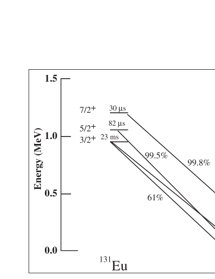
FIG. 1.: Proton emission from the [411]3/2 rotational band in ¹³¹Eu calculated in the non-adiabatic model. Half-lives for proton emission and branching ratios are indicated.

The calculation of branching ratios (b.r.) is straightforward in the non-adiabatic formalism. The partial width corresponding to the $J$$\rightarrow$$J_{d}$ decay is given by $\Gamma(J\rightarrow J_{d})=\sum_{j_{p}l_{p}}\Gamma^{J}_{J_{d}j_{p}l_{p}}$ It is seen that the proton-emission lifetimes and b.r. change with $J$. Of course, at the low energies shown in Fig. 1, rotational states decay by emitting gamma radiation ($\Gamma_{\gamma}$$\gg$$\Gamma_{p}$). (The competition with proton emission is expected to take place at higher energies/spins.) The 3/2⁺$\rightarrow$0⁺ decay is given by the very small $d_{3/2}$ component. The large branching to the 2⁺ state is due to the dominating $d_{5/2}$ partial wave. (This also explains the fact that the 5/2⁺ level decays predominantly to the 0⁺ ground state.) It is worth noting that the $s_{1/2}$ component, not allowed in the adiabatic approach due to $K$-conservation, also contributes to the 3/2⁺$\rightarrow$2⁺ transition. Although $K$ is not conserved in the non-adiabatic approach, one can decompose the wave function into states (7) with definite $K$. In most cases, we find that one $K$-component dominates the wave function. Consequently, the Nilsson labeling convention can still be used.

Transitions to excited daughter states, $K$$\rightarrow$$J_{d}$, may also be approximated in the strong coupling framework [7, 9]. In this case the angular momentum conservation is guaranteed by the presence of the geometric factor $(C_{KK,K-K}^{J_{d}0})^{2}$. In addition, the $Q_{p}$ value is adjusted to $Q_{J_{d}}$.

As shown previously in Ref. [5], at large deformations our calculations show a very small dependence on $\beta_{2}$ and $\beta_{4}$. This is because the spherical decomposition of the corresponding Nilsson orbitals varies little in this regime, and there are no crossings between the levels of interest. The uncertainty due to the $\beta_{2}$ value is usually much smaller than the experimental uncertainty in the proton energy. Table I shows predicted half-lives and b.r. for ¹³¹Eu and ¹⁴¹Ho. For ¹³¹Eu we take $\beta_{2}=0.32$ and for ¹⁴¹Ho ($\beta_{2}=0.29,\beta_{4}=-0.06$) [5]. Spectroscopic factors have been estimated in the independent-quasiparticle picture. Note that the $1/(\Omega+1/2)$ coefficient multiplying the BCS values of $u^{2}$, assumed in Ref. [5], is no longer present.

	Orbital	$u^{2}$	$\tau_{1/2}$	b.r. (nad)	b.r. (ad)
	$[411]{\scriptstyle{\frac{3}{2}}}$	0.71	34.0 ms	39%	37%
131Eu	$[413]{\scriptstyle{\frac{5}{2}}}$	0.52	184 ms	7%	2%
	$[532]{\scriptstyle{\frac{5}{2}}}$	0.48	3.90 s	52%	38%
			17.8(19) ms	24(5) %
141Ho	$[523]{\scriptstyle{\frac{7}{2}}}$	0.84	19.1 ms	6%	3%
			3.9(5) ms
141mHo	$[411]{\scriptstyle{\frac{1}{2}}}$	0.70	3.3 $\mu$s	1%	1%
			8(3) $\mu$s

TABLE I.: Half-lives and branching ratios (b.r.) to the $J_{d}^{+}$=$2^{+}$ state for deformed proton resonances in ¹³¹Eu and ¹⁴¹Ho calculated in the non-adiabatic (nad) and adiabatic (ad) formalism. The experimental values (shown in boldface) are taken from Refs. [7, 5]. The energy of the 2⁺ state in ¹³⁰Sm and ¹⁴⁰Dy was assumed to be 120 keV and 160 keV, respectively.

Considering both the half-life and b.r., the ground state of ¹³¹Eu is consistent with the $[411]3/2$ assignment. This result agrees with the analysis of Ref. [7] and is at variance with the suggestion by Maglione et al. who assigned the [413]5/2 orbital as a ground state of ¹³¹Eu. The very small b.r. for the [413]5/2 orbital results from the fact that both the 5/2⁺$\rightarrow$0⁺ and 5/2⁺$\rightarrow$2⁺ transitions go via the $d_{5/2}$ component which constitutes about 4% of the wave function. On the other hand, for the yet-unobserved [532]5/2 state, the 5/2^-$\rightarrow$0⁺ transition goes via the tiny (0.1%) $f_{5/2}$ wave, while the 5/2^-$\rightarrow$2⁺ decay is dominated by the $f_{7/2}$ component (17%) and the $K$-forbidden $p_{3/2}$ wave, which appears due to the Coriolis coupling. This results in the huge branching predicted for this state.

For ¹⁴¹Ho, based on calculated half-lives, we can assign the $[523]7/2$ level to the ground state and $[411]1/2$ to the excited state. We note that these assignments are identical to our previous assignment in Ref. [5], although we are now using the non-adiabatic formalism and have changed the optical model parameters. These assignments also agree with those proposed in Refs. [3, 13].

For ¹⁴⁰Dy, the energy of the $2^{+}$ state is experimentally unknown, but it can be estimated from systematic trends. For instance, according to the $N_{p}N_{n}$ scheme, one obtains the value $E_{2^{+}}$=160 keV [28], which was adopted in the calculations displayed in Table I. Figure 2 shows the expected b.r. to the $2^{+}$ state as a function of $E_{2^{+}}$ for both proton-emitting states in ¹⁴¹Ho. For the [523]7/2 ground state, the predicted b.r. is still of the order of a few percent even at relatively large values of $E_{2^{+}}$, and this offers good prospects for its experimental observation. On the other hand, the b.r. for the isomeric [411]1/2 state is lower by an order of magnitude.

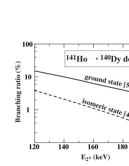
FIG. 2.: Predicted branching ratio for the proton transition from $J^{\pi}$=7/2^- and 1/2⁺ states in ¹⁴¹Ho to the $2^{+}$ state in ¹⁴⁰Dy as a function of $E_{2^{+}}$. The expected value of $E_{2^{+}}$ is around 160 keV.

In ¹³¹Eu the experimental uncertainty in the $Q_{p}$ value leads to an uncertainty of $+30\%$ / $-22\%$ for all three levels. The branching ratios vary by less than $3\%$.

In conclusion, we applied a non-adiabatic formalism, based on the coupled-channel Schrödinger equation with outgoing wave boundary conditions, to describe very narrow proton resonances in deformed nuclei. The non-adiabatic model takes into account the fact that the daughter nucleus has a finite moment of inertia. Our calculations are consistent with the experimental data for the best deformed proton emitters known so far: ¹³¹Eu and ¹⁴¹Ho. As shown in Table I, the adiabatic approximation gives rise to an underestimation of branching ratios sometimes by a factor 2-3. According to our predictions, there is a good chance to study experimentally the fine structure in the proton decay of ¹⁴¹Ho.

- [1] S. Hofmann, Radiochim. Acta 70/71, 93 (1995).
- [2] P.J. Woods and C.N. Davids, Ann. Rev. Nucl. Part. Sci. 47, 541 (1997).
- [3] C.N. Davids et al., Phys. Rev. Lett. 80, 1849 (1998).
- [4] J.C. Batchelder et al., Phys. Rev. C57, R1042 (1998).
- [5] K. Rykaczewski et al., Phys. Rev. C 60, 011301 (1999).
- [6] C.R. Bingham et al., Phys. Rev. C 59, R2984 (1999).
- [7] A.A. Sonzogni et al., Phys. Rev. Lett. 83, 1116 (1999).
- [8] S. Åberg, P.B. Semmes, and W. Nazarewicz, Phys. Rev. C 56, 1762 (1997).
- [9] V.P. Bugrov and S.G. Kadmenskiĭ, Sov. J. Nucl. Phys. 49, 967 (1989); S.G. Kadmenskiĭ and V.P. Bugrov, Phys. Atomic Nuclei 59, 399 (1996).
- [10] S.G. Kadmenskiĭ, V.E. Kalechtis, and A.A. Martynov, Sov. J. Nucl. Phys. 14, 193 (1972); S.G. Kadmenskiĭ and V.G. Khlebostroev, Sov. J. Nucl. Phys. 18, 505 (1974).
- [11] L.S. Ferreira, E. Maglione, and R.J. Liotta, Phys. Rev. Lett. 78, 1640 (1997).
- [12] E. Maglione, L.S. Ferreira, and R.J. Liotta, Phys. Rev. Lett. 81, 538 (1998).
- [13] E. Maglione, L.S. Ferreira, and R.J. Liotta, Phys. Rev. C 59, R589 (1999).
- [14] P. Talou, N. Carjan, and D. Strottman, Phys. Rev. C58, 3280 (1998).
- [15] J. Humblet and L. Rosenfeld, Nucl. Phys. 26, 529 (1961).
- [16] T. Tamura, Rev. Mod. Phys. 67, 679 (1965).
- [17] S. Ćwiok, J. Dudek, W. Nazarewicz, J. Skalski, and T. Werner, Comput. Phys. Commun. 46, 379 (1987).
- [18] V.A. Chepurnov, Yad. Fiz. 6, 955 (1967); Sov. J. Nucl. Phys. 7, 715 (1968).
- [19] F.D. Becchetti, Jr. and G.W. Greenlees, Phys. Rev. 182, 1190 (1969).
- [20] W. Nazarewicz, M.A. Riley, and J.D. Garrett, Nucl. Phys. A512, 61 (1990).
- [21] J. Dudek, Z. Szymański, and T. Werner, Phys. Rev. C23, 920 (1981).
- [22] S.G. Nilsson, Mat. Fys. Medd. Dan. Vid. Selsk. 29, No. 16 (1955).
- [23] B. Gyarmati and T. Vertse, Nucl. Phys. A160, 523 (1971).
- [24] B. Simon, Phys. Lett. 73A, 211 (1979).
- [25] L.Gr. Ixaru, Numerical Methods for Differential Equations, (Reidel, Dordrecht-Boston-Lancaster, 1984).
- [26] T. Vertse, A.T. Kruppa, L.Gr. Ixaru, and M. Rizea, in preparation.
- [27] B.C. Barrett, Nucl. Phys. 51, 27 (1964).
- [28] N.V. Zamfir, private communication, 1999.