The Role of Meson Retardation in the $NN$ Interaction above Pion Threshold

Abstract

A model is developed for the hadronic interaction in the two-nucleon system above pion threshold which is based on meson, nucleon and $\Delta$ degrees of freedom and which includes full meson retardation in the exchange operators. For technical reasons, the model allows maximal one meson to be present explicitly. Thus the Hilbert space contains besides $NN$ and $N\Delta$ also configurations consisting of two nucleons and one meson. For this reason, only two- and three-body unitarity is obeyed, and the model is suited for reactions in the two nucleon sector, where only one pion is produced or absorbed. Starting from a realistic pure nucleonic retarded potential, which had to be renormalized because of the additional $\pi$ and $\Delta$ degrees of freedom, a reasonable fit to experimental $NN$ scattering data could be achieved.

I Introduction

At present a very interesting topic in the field of medium energy physics is devoted to the role of effective degrees of freedom (d.o.f.) in hadronic systems in terms of nucleon, meson and isobar d.o.f. and their connection to the underlying quark-gluon dynamics of QCD. For the study of this basic question, the two-nucleon system provides an important test laboratory, because it is obviously the simplest nuclear system for the study of the nucleon-nucleon interaction in $NN$ scattering including deuteron properties, and, furthermore, for testing this effective description in other reactions on the deuteron, for example, in elastic and inelastic electron scattering, in photodisintegration, and meson photo- and electroproduction. Moreover, due to the lack of free neutron targets, reactions on the deuteron are also an important tool to test our present understanding of neutron properties. As an example for the latter aspect, we would like to mention the recently much discussed determination of the electric form factor $G_{E,n}$ of the neutron in $d(\vec{e},e^{\prime}\vec{n})p$ [1] and $\vec{d}(\vec{e},e^{\prime}n)p$ [2], or the investigation of the Gerasimov-Drell-Hearn sum rule for the deuteron [3]. However, in order to separate the unwanted binding effects from the neutron properties, a precise knowledge of the structure dependent effects is needed.

Intense efforts over many past decades in experiment and theory have shown that for energies below pion threshold a satisfactory description of $NN$ scattering and deuteron properties [4, 5], as well as photo- and electrodisintegration of the deuteron is achieved within the conventional framework of nucleon, meson and isobar d.o.f. [6, 7], although the description of observables is not perfect because for certain observables significant discrepancies remain unresolved as, for example, in elastic electron deuteron scattering [8]. At higher energies, above pion threshold our theoretical understanding of the various experimental data is much less well settled. Even for deuteron photodisintegration (for a detailed review see [6]), none of the various theoretical approaches like the diagrammatic method of Laget [9], the framework of nuclear isobar configurations in the impulse approximation [10], the unitary three-body model [11] or the coupled channel approach (CC) [12, 13] is able to describe in a satisfactory manner the whole set of experimental data on differential cross sections and polarization observables for energies covering the whole $\Delta$ resonance region.

A common feature of most of these approaches is the extensive use of the static limit for the meson propagator which enters the hadronic interaction and the electromagnetic two-body exchange current operators, although there is little justification for that in view of the relatively high excitation energies involved. Also from the point of view of special relativity, a non-instantaneous interaction would be required. The reason, why this static approximation is still used, is the enormous simplification of the operator structure becoming local, and thus is much simpler to evaluate numerically. It has already been conjectured in [13], that one main reason for the above mentioned failure of the theoretical description lies in the neglect of meson retardation in the meson exchange operators. Indeed, first results [14, 15] based on the thesis of M. Schwamb [16] have shown that a much better description of deuteron photodisintegration compared to the static approaches is obtained if meson retardation is retained.

In this paper, we want to present a realistic, but still tractable model for a retarded hadronic interaction within a nonrelativistic framework which is suitable to be used as input in electromagnetic reactions on the deuteron like, for example, photo- and electrodisintegration or pion production. There exists already a variety of models for treating retardation in $NN$ scattering based on three-body theory, for example, the work of Kloet and Silbar [17] and Tanabe and Ohta [18]. In these calculations, however, the driving force is basically one-pion-exchange so that the lower partial waves in $NN$ scattering cannot be described reasonably well, even at energies below pion threshold. The neglected short-range interaction is, however, of crucial importance for electromagnetic and hadronic breakup reactions on the deuteron. Tanabe and Ohta, for example, have ”patched up” this problem in photodisintegration of the deuteron [11] by mixing retarded and static frameworks, namely the static Paris potential for the final state interaction with respect to the nucleon one-body current and the $\pi$ MEC, whereas for the $\Delta$ contributions they employ a three-body model in which heavy meson exchange has been neglected. Kloet and Silbar on the other hand have taken a retarded pion exchange and static heavy meson exchange in an improved model of $NN$ scattering [19]. Also other treatments of retardation in the $NN$-interaction like, e.g. Refs. [22, 23] have some drawbacks as will be discussed later. The shortcomings of these approaches have been overcome to a large extent in the present model which ensures, due to the use of the Elster-Potential [20, 21] as an input, a reasonable description of all relevant partial waves below and above pion threshold within a consistent framework in time-ordered perturbation theory.

Thus we will present here the basic framework of a model for the hadronic interaction in which retardation in the exchange operators is fully included. We would like to emphasize the fact that this formalism can be applied to any reaction on the two-nucleon system for excitation energies up to about 500 MeV in which not more than one pion is produced or absorbed. But in this paper we will restrict ourselves to the hadronic interaction in studying $NN$ scattering and deuteron properties only in order to fix all free hadronic parameters of our model. The application of this formalism to other hadronic reactions like $\pi d$ scattering as well as to electromagnetic reactions will be deferred to forthcoming papers.

The conceptual basis and the main features of our model are laid out in Sect. II. In view of the fact that conventional retarded interactions in pure nucleonic space are energy dependent and thus non-hermitean, we enlarge the Hilbert space by considering explicitly meson and $\Delta$ d.o.f. in order to start with a hermitean hamiltonian. The retarded interaction is then generated by meson-nucleon and $\pi N\Delta$ vertices. For reasons of simplicity, we restrict ourselves in this work to configurations with only one meson present besides the baryons. Special attention is laid on the question of nucleon dressing and the corresponding renormalization of operators as well as the fulfilment of two- and three-body unitarity. With respect to the latter, we have incorporated the $\pi d$ channel in a realistic model showing some interesting effects. The $NN$ scattering $T$ matrix is derived, and the structure of the deuteron is discussed. A field theoretical realization in the form of a one-boson-exchange model is developed in Sect. III with inclusion of the $\Delta$ isobar which is conceptually similar to the work of the Bonn group [24] but differs in some essential details. Then we will present and discuss in Sect. IV the results for $NN$ scattering comparing them with experiment as well as with other theoretical approaches. Finally, Sect. V contains a summary and an outlook.

II Basic considerations

A The Hilbert space

Our model for the description of a nuclear system allows besides $n$ nucleons configurations with one additional meson present or where one nucleon is replaced by a $\Delta$ isobar. It is similar (but not identical) to the approach of Sauer and collaborators [23, 25, 26, 27] which is also used in [13, 28, 29]. Thus the model Hilbert space ${\cal H}^{[n]}$ is subdivided into three orthogonal spaces according to the different configurations containing either $n$ bare nucleons $({\cal H}^{[n]}_{\bar{N}})$, $n-1$ nucleons and one $\Delta$ (${\cal H}^{[n]}_{\Delta})$, or $n$ nucleons and one meson $({\cal H}^{[n]}_{X})$, i.e.

$${\cal H}^{[n]}={\cal H}^{[n]}_{\bar{N}}\oplus{\cal H}^{[n]}_{\Delta}\oplus{\cal H}^{[n]}_{X}\,.$$ (1)

The “bar” indicates a bare nucleon to be distinguished from the corresponding physical nucleon, denoted without a bar. This distinction is necessary in order to take into account the dressing of a bare nucleon by meson-nucleon loops. For the $\Delta$ isobar we will not make this distinction, because the self energy contributions from $\pi N$ loops will be retained explicitly, whereas the dressing of the bare nucleon to become a physical nucleon will be incorporated into the effective operators by dressing factors. In ${\cal H}^{[n]}_{X}$ only one meson is present besides $n$ nucleons, i.e., no components with two or more mesons are taken into account (one-meson-approximation). This limitation creates some pathologies as will be pointed out later. In detail it means

$${\cal H}^{[n]}_{X}=\bigoplus\limits_{x\in\{\pi,\,\eta,\,\sigma,\,\delta,\,\omega,\,\rho\}}{\cal H}^{[n]}_{x}\,,$$ (2)

considering as mesons $\pi$, $\eta$, $\sigma$, $\delta$, $\omega$, and $\rho$.

In order to distinguish the various sectors of ${\cal H}^{[n]}$, we introduce corresponding projection operators by

$$P_{{\bar{N}}}{\cal H}^{[n]}={\cal H}^{[n]}_{\bar{N}}\,,\qquad P_{\Delta}{\cal H}^{[n]}={\cal H}^{[n]}_{\Delta}\,,\qquad P_{X}{\cal H}^{[n]}={\cal H}^{[n]}_{X}\,,\mbox{ and }P=P_{\bar{N}}+P_{\Delta}\,.$$ (3)

The latter is introduced since later we also will need the projection operator on the combined pure baryon subspace ${\cal H}^{[n]}_{\bar{N}}\oplus{\cal H}^{[n]}_{\Delta}$. Moreover, in view of the different subspaces in the meson-nucleon sector, it is useful to decompose the projection operator $P_{X}$ into a sum of six orthogonal projectors corresponding to the six mesons considered

$$P_{X}=\sum_{x\in\{\pi,\,\eta,\,\sigma,\,\delta,\,\omega,\,\rho\}}P_{x}\,\mbox{ with }P_{x}{\cal H}^{[n]}={\cal H}^{[n]}_{x}\,\mbox{ for }x\in\{\pi,\eta,\sigma,\delta,\omega,\rho\}\,.$$ (4)

Using the notation

$$\Omega_{\alpha\beta}=P_{\alpha}\Omega P_{\beta}\,,\qquad\alpha,\,\beta\in\{\bar{N},\,\Delta,\,X\}\,,$$ (5)

any operator $\Omega$ acting in ${\cal H}^{[n]}$ can be written as a symbolic $3\times 3$ matrix

$$\Omega=\left(\begin{array}[]{ccc}\Omega_{{\bar{N}}{\bar{N}}}&\Omega_{{\bar{N}}\Delta}&\Omega_{{\bar{N}}X}\\ \Omega_{\Delta{\bar{N}}}&\Omega_{\Delta\Delta}&\Omega_{\Delta X}\\ \Omega_{X{\bar{N}}}&\Omega_{X\Delta}&\Omega_{XX}\end{array}\right).$$ (6)

B The Hamiltonian

The Hamilton operator $H$ of the model can be divided into a diagonal kinetic part and an interaction describing the emission and absorption of a meson by a baryon and, in addition, an ab initio baryon-baryon interaction

$$H=\bar{H}_{0}+H_{I}\,,$$ (7)

where the bar indicates that it refers to bare baryons. In particular, the nucleon kinetic energies are determined by the bare nucleon mass $M_{\bar{N}}$. However, due to the truncation of the Hilbert space with respect to the number of mesons, no explicit dressing of the bare nucleons is possible in ${\cal H}^{[n]}_{\Delta}\oplus{\cal H}^{[n]}_{X}$. This is one of the pathologies which one encounters in the one-meson-approximation. Therefore, we will use the physical instead of the bare nucleon mass in ${\cal H}^{[n]}_{\Delta}\oplus{\cal H}^{[n]}_{X}$, so that the formally suppressed meson-nucleon loops can be taken into account at least effectively by the physical nucleon mass. For simplicity, we use in ${\cal H}^{[n]}_{\Delta}$ the nonrelativistic expressions for the kinetic energies of nucleon and $\Delta$ isobar because we will treat the $\Delta$ nonrelativistically. This approximation is, however, not crucial. For later purposes we will introduce as kinetic energy in addition a second type of one-body operator $H_{0}$ which differs from $\bar{H}_{0}$ in the pure nucleonic sector only, referring to physical nucleon kinetic energies also in ${\cal H}^{[n]}_{\bar{N}}$. Thus we have in detail

$$\bar{H}_{0,\,{\bar{N}}{\bar{N}}} = \sum_{j=1}^{n}{h}_{\bar{N}}(j)\,,$$ (8)

$$H_{0,\,{\bar{N}}{\bar{N}}} = \sum_{j=1}^{n}{h}_{N}(j)\,,$$ (9)

$$\bar{H}_{0,\,\Delta\Delta} = H_{0,\,\Delta\Delta}=\sum_{j=1}^{n-1}{h}^{nr}_{N}(j)+{h}_{\Delta}\,,$$ (10)

$$\bar{H}_{0,\,XX} = H_{0,\,XX}=\sum_{j=1}^{n}{h}_{N}(j)+{h}_{X}\,,$$ (11)

with the various kinetic energies (with masses $m_{x},x\in\{\pi,\,\eta,\,\sigma,\,\delta,\,\omega,\,\rho\}$, $M^{0}_{\Delta}$, $M_{\bar{N}}$ and $M_{N}$, respectively)

$$\mbox{$\langle{\bar{N}}(\vec{p}^{\,\prime})|$}{h}_{\bar{N}}\mbox{$|{\bar{N}}(\vec{p}\,)\rangle$}=e_{\bar{N}}(p)\,\delta\left(\vec{p}^{\,\prime}-\vec{p}\,\right)\,, e_{\bar{N}}(p)=\sqrt{{M^{2}_{\bar{N}}}+p^{2}}\,,$$ (12)

$$\mbox{$\langle{\bar{N}}(\vec{p}^{\,\prime})|$}{h}_{N}\mbox{$|{\bar{N}}(\vec{p}\,)\rangle$}=e_{N}(p)\,\delta\left(\vec{p}^{\,\prime}-\vec{p}\,\right)\,, e_{N}(p)=\sqrt{M^{2}_{N}+p^{2}}\,,$$ (13)

$$\mbox{$\langle{\bar{N}}(\vec{p}^{\,\prime})|$}{h}^{nr}_{N}\mbox{$|{\bar{N}}(\vec{p}\,)\rangle$}=e^{nr}_{N}(p)\,\delta\left(\vec{p}^{\,\prime}-\vec{p}\,\right)\,, e^{nr}_{N}(p)=M_{N}+\frac{p^{2}}{2M_{N}}\,,$$ (14)

$$\mbox{$\langle\Delta(\vec{p}^{\,\prime})|$}{h}_{\Delta}\mbox{$|\Delta(\vec{p}\,)\rangle$}=e_{\Delta}(p)\,\delta\left(\vec{p}^{\,\prime}-\vec{p}\,\right)\,, e_{\Delta}(p)=M^{0}_{\Delta}+\frac{p^{2}}{2M^{0}_{\Delta}}\,,$$ (15)

$$\mbox{$\langle x(\vec{q}^{\,\prime})|$}{h}_{x}\mbox{$|x(\vec{q}\,)\rangle$}=(2\pi)^{3}\,2\,\omega_{x}(q)\,\delta\left(\vec{q}^{\,\prime}-\vec{q}\,\right)\,, \omega_{x}(p)=\sqrt{m_{x}^{2}+p^{2}}\,,\quad\mbox{for}\,\,x\in\left\{\pi,\eta,\sigma,\delta,\omega,\rho\right\}\,.$$ (16)

In view of the two choices for the kinetic energy, one obtains besides the interaction $H_{I}$, defined in (7) another interaction operator $V^{0}$ as defined via

$$H=H_{0}+V^{0}\,.$$ (17)

The various components of the interaction $V^{0}$ are depicted in Fig. 1. First of all, $V^{0}$ contains, because of

$$V^{0}=H_{I}+\bar{H}_{0}-H_{0}\,,$$ (18)

besides the interaction $H_{I}$, a diagonal counter term

$$V^{[c]}=\bar{H}_{0}-H_{0}\,,$$ (19)

which is nonzero in ${\cal H}^{[n]}_{\bar{N}}$ only, and which is a pure one-body operator

$$V^{[c]}_{\bar{N}\bar{N}}=\sum_{j=1}^{n}v^{[c]}_{\bar{N}\bar{N}}(j)\,,\mbox{ with }v^{[c]}_{\bar{N}\bar{N}}={h}_{\bar{N}}-{h}_{N}\,.$$ (20)

As already mentioned, we allow in addition in $V^{0}_{PP}$ a two-body part $V^{0\,[2]}_{PP}$ which describes an ab initio given hermitean interaction between two baryons, i.e.,

$$V^{0}_{PP}=V^{[c]}_{PP}+V^{0\,[2]}_{PP}\,,$$ (21)

which will be specified later. The nondiagonal components $V^{0}_{X{\bar{N}}}$ and $V^{0}_{X\Delta}$ are one-body operators

$$V^{0}_{X{\bar{N}}} = \sum_{j=1}^{n}v^{0}_{X{\bar{N}}}(j)\,,\quad V^{0}_{X\Delta}=\sum_{j=1}^{n}v^{0}_{X\Delta}(j)\,,$$ (22)

describing the emission of a meson by a baryon. The remaining interaction $V^{0}_{XX}$ consists in the one-meson-approximation in principle of two parts

$$V^{0}_{XX}=V^{0\,\bar{N}}_{XX}+\sum_{x\in\{\pi,\,\eta,\,\sigma,\,\delta,\,\omega,\,\rho\}}V^{0\,x}_{XX}\,.$$ (23)

The first one describes a meson-nucleon interaction with the other nucleons as spectators and the second one two interacting nucleons with a meson $x$ and the remaining nucleons as spectators (see Fig. 1). In consequence, $V^{0\,{\bar{N}}}_{XX}$ is a one-body operator

$$V^{0\,{\bar{N}}}_{XX}=\sum_{i=1,2}v^{0}_{XX}(i)\,.$$ (24)

In the previous work of Wilhelm et al. [13, 28, 29] and Bulla et al. [23], $V^{0}_{XX}$ was neglected completely for practical reasons. Above the $\pi d$ threshold, however, this approximation leads to several problems, in particular for three-body unitarity (see the discussion in Sect. III D), which are solely due to the neglect of $V^{0\,\pi}_{XX}$. We therefore set

$$V^{0\,{\bar{N}}}_{XX}\equiv 0\,,$$ (25)

and for $x\neq\pi$

$$V^{0\,x}_{XX}\equiv 0\,,$$ (26)

whereas only $V^{0\,\pi}_{XX}$ will be retained nonzero.

C $NN$ scattering

Now we will consider $NN$ scattering in the two-nucleon sector. The renormalization of a free nucleon state $|N;\,\vec{p}\,\rangle$ is sketched briefly in Appendix A. The scattering states of two physical nucleons $\mbox{$|NN;\,\vec{p},\alpha\rangle$}^{(\pm)}$ in the c.m. system with the asymptotic free relative momentum $\vec{p}$, energy $E^{NN}_{p}=2e_{N}(p)$ and a complete set of internal quantum numbers $\alpha$ are given by

$$\mbox{$|NN;\,\vec{p},\alpha\,\rangle$}^{(\pm)}=N_{[2]}^{-1}(\vec{p}\,)\Big{(}1+G_{0}(E^{NN}_{p}\pm i\epsilon)T^{0}(E^{NN}_{p}\pm i\epsilon)\Big{)}\mbox{$|\bar{N}\bar{N};\,\vec{p},\alpha\rangle$}\,,$$ (27)

where $N_{[2]}(\vec{p}\,)$ is a renormalization constant which appears because both, the bare as well as the physical free two-nucleon states are normalized to the $\delta$ function. The transition amplitude $T^{0}$ satisfies the Lippmann-Schwinger equation

$$T^{0}(z) = V^{0}+V^{0}G_{0}(z)T^{0}(z)\,\,$$ (28)

with the free propagator $G_{0}$

$$G_{0}(z)=(z-H_{0})^{-1}\,,$$ (29)

which is represented in Fig. 2. As is shown in detail in the Appendix B, one finds for the $T$ matrix element

$$\mbox{$\langle NN;\,\vec{p}^{\,\prime},\alpha^{\prime}|$}T(E^{NN}_{p}+i\epsilon)\mbox{$|NN;\,\vec{p},\alpha\rangle$} = N_{[2]}^{-2}(p)\mbox{$\langle{\bar{N}}{\bar{N}};\,\vec{p}^{\,\prime},\alpha^{\prime}|$}T^{0}(E^{NN}_{p}+i\epsilon)\mbox{$|{\bar{N}}{\bar{N}};\,\vec{p},\alpha\rangle$}$$ (30)

$$= \mbox{$\langle{\bar{N}}{\bar{N}};\,\vec{p}^{\,\prime},\alpha^{\prime}|$}T^{con}_{{\bar{N}}{\bar{N}}}(E^{NN}_{p}+i\epsilon))\mbox{$|{\bar{N}}{\bar{N}};\,\vec{p},\alpha\rangle$}\,.$$ (31)

Here, $T^{con}$ - the superscript “$con$” refers to connected diagrams (see Appendix B) - obeys a Lippmann-Schwinger equation

$$T^{con}_{PP}(z)={\widehat{R}}(z)\,V^{con}_{PP}(z)\,{\widehat{R}}(z)+{\widehat{R}}(z)\,V^{con}_{PP}(z)\,{\widehat{R}}(z)\,G_{0}(z)\,T^{con}_{PP}(z)\,.$$ (32)

Its driving term contains a “renormalized” interaction

$$V^{con}_{PP}(z) = ({\widehat{Z}}_{[2]}^{os})^{-1}\,V^{0,\,con}_{PP}(z)\,({\widehat{Z}}_{[2]}^{os})^{-1}\,,$$ (33)

where $V^{0,\,con}_{PP}$, as defined in Appendix B, comprises besides $\pi N$ loop contributions to the $\Delta$ self energy the genuine retarded baryon-baryon interaction. Its diagrammatic representation is shown in Fig. 3. Furthermore, the “dressing operator” is given by

$${\widehat{R}}(z)={\widehat{Z}}_{[2]}^{os}\,{\widehat{Z}}_{[2]}^{-1}(z)\,.$$ (34)

Here the two-body renormalization operator ${\widehat{Z}}_{[2]}$ is defined as

$${\widehat{Z}}^{2}_{[2]}(z) = 1+\int dz^{\prime}\,\delta(z^{\prime}-H_{0})\,\left[V^{0}_{{\bar{N}}X}\,G_{0}(z^{\prime})\,G_{0}(z)\,V^{0}_{X{\bar{N}}}\right]_{dis}\,,$$ (35)

where the subscript “$dis$” refers to disconnected diagrams (see Appendix B), and which differs from unity in ${\cal H}^{[2]}_{\bar{N}}$ only. Its onshell value is

$$({\widehat{Z}}^{os}_{[2]})^{2} = 1+\int dz^{\prime}\,\delta(z^{\prime}-H_{0})\,\left[V^{0}_{{\bar{N}}X}\,G_{0}(z^{\prime})\,G_{0}(z^{\prime})\,V^{0}_{X{\bar{N}}}\right]_{dis}\,.$$ (36)

Thus $NN$ scattering is unambiguously fixed by the onshell matrix element of $T^{con}_{{\bar{N}}{\bar{N}}}$.

For later applications we need also the offshell form of $T^{con}_{PP}(z)$ for which one finds the following expression

$$T^{con}_{PP}(z)=G_{0}^{-1}(z)\left\{G_{0}^{(\Delta)}(z)+G_{0}^{(\Delta)}(z){\widetilde{T}}^{con}_{PP}(z)G_{0}^{(\Delta)}(z)\right\}G_{0}^{-1}(z)-G_{0}^{-1}(z)\,.$$ (37)

The auxiliary amplitude ${\widetilde{T}}^{con}_{PP}(z)$ is given by the integral equation

$${\widetilde{T}}^{con}_{PP}(z)=V^{con}_{[2]\,PP}(z)+V^{con}_{[2]\,PP}(z)G_{0}^{(\Delta)}(z){\widetilde{T}}^{con}_{PP}(z)\,,$$ (38)

where the driving terms $V^{con}_{[i]\,PP}(z)$ ($i=1,2$) are defined by separating in $V^{con}_{PP}(z)$ the $\pi N$ loop contributions to the $\Delta$ self energy, subdividing it into two parts

$$V^{con}_{PP}(z)=V^{con}_{[1]\,PP}(z)+V^{con}_{[2]\,PP}(z)\,,$$ (39)

where

$$V^{con}_{[1]\,PP}(z) = \left[V_{\Delta X}G_{0}(z)V_{X\Delta}\right]_{dis}\,,$$ (40)

$$V^{con}_{[2]\,PP}(z) = V^{[2]}_{PP}+\left[V_{PX}G_{0}(z)V_{XP}\right]_{con}+V_{PX}G_{0}(z)T^{X}(z)G_{0}(z)V_{XP}\,,$$ (41)

with the renormalized interactions

$$V^{[2]}_{PP} = ({\widehat{Z}}_{[2]}^{os})^{-1}\,V_{PP}^{0\,[2]}\,({\widehat{Z}}_{[2]}^{os})^{-1}\,,$$ (42)

$$V_{XP} = ({\widehat{Z}}_{[2]}^{os})^{-1}\,V_{XP}^{0}\,({\widehat{Z}}_{[2]}^{os})^{-1}\,.$$ (43)

Here, $T^{X}(z)$ is the $NN$ scattering matrix in the presence of a spectator meson fulfilling

$$T^{X}(z)=V^{0}_{XX}+V^{0}_{XX}\,G_{0}(z)\,T^{X}(z)\,.$$ (44)

Its diagrammatic representation is shown in Fig. 4. Thus the term $V^{con}_{[1]\,PP}(z)$ contains solely the intermediate $\pi N$ loop contributions to the $\Delta$ propagator. Furthermore, we have introduced in (37) a “dressed” propagator

$$G_{0}^{(\Delta)}(z)=G_{0}(z)+G_{0}(z)V^{con}_{[1]\,PP}(z)G_{0}^{(\Delta)}(z)\,,$$ (45)

which takes into account the dressing of the $\Delta$ in ${\cal H}^{[2]}_{\Delta}$. In ${\cal H}^{[2]}_{\bar{N}}$ and ${\cal H}^{[2]}_{X}$, $G_{0}^{(\Delta)}(z)$ is identical to the free propagator, whereas in ${\cal H}^{[2]}_{\Delta}$ one gets a simple connection between $G_{0}^{(\Delta)}(z)$ and the $\Delta$ propagator $g_{\Delta}(z)$ in the one-$\Delta$ sector (see Sect. III B)

$$\mbox{$\langle{\bar{N}}\Delta;\,\vec{p}^{\,\prime}|$}G_{0\Delta\Delta}^{(\Delta)}(z)\mbox{$|{\bar{N}}\Delta;\,\vec{p}\,\rangle$}=\mbox{$\langle\Delta;\,\vec{p}^{\,\prime}|$}g_{\Delta}\left(z-M_{N}-\frac{\vec{p}^{\,2}}{2\mu_{N\Delta}}\right)\mbox{$|\Delta;\,\vec{p}\,\rangle$}\,,$$ (46)

where $\vec{p}$ is the relative momentum of the $\bar{N}\Delta$ system, and its reduced mass is denoted by

$$\mu_{N\Delta}=\frac{M^{0}_{\Delta}M_{N}}{M^{0}_{\Delta}+M_{N}}\,.$$ (47)

In addition, we need the baryonic and mesonic components of the $NN$ scattering states for which one finds

$$P_{\bar{N}}\mbox{$|NN;\,\vec{p},\,\alpha\rangle$}^{(\pm)} = \frac{{\widehat{R}}(z)}{{\widehat{Z}}^{os}_{[2]}}\left(1+G_{0}(z){\widetilde{T}}^{con}_{\bar{N}\bar{N}}(z)\right)\mbox{$|\bar{N}\bar{N};\,\vec{p},\,\alpha\rangle$}\,,$$ (48)

$$P_{\Delta}\mbox{$|NN;\,\vec{p},\,\alpha\rangle$}^{(\pm)} = G_{0}^{(\Delta)}(z){\widetilde{T}}^{con}_{\Delta\bar{N}}(z)\mbox{$|\bar{N}\bar{N};\,\vec{p},\,\alpha\rangle$}\,,$$ (49)

$$P_{X}\mbox{$|NN;\,\vec{p},\,\alpha\rangle$}^{(\pm)} = G^{X}(z)\Big{(}V_{X\bar{N}}\,{\widehat{Z}}^{os}_{[2]}+V_{X\Delta}\Big{)}\mbox{$|NN;\,\vec{p},\,\alpha\rangle$}\,,$$ (50)

where $z=E^{NN}_{p}\pm i\epsilon$, and $G^{X}(z)$ describes the propagation of two interacting nucleons in the presence of a spectator meson

$$G^{X}(z) = (z-H_{0,\,XX}-V^{0}_{XX})^{-1}$$ (51)

$$= G_{0}(z)+G_{0}(z)\,T^{X}(z)\,G_{0}(z)\,.$$ (52)

D The deuteron

Due to its vanishing isospin, the deuteron cannot contain a $\bar{N}\Delta$ component. Thus, the deuteron state $|\bar{d}\rangle$ can be separated into a nucleonic and a mesonic component

$$\mbox{$|\bar{d}\rangle$}=P_{\bar{N}}\mbox{$|\bar{d}\rangle$}+P_{X}\mbox{$|\bar{d}\rangle$}\,,$$ (53)

which can be determined by the Schrödinger equation in the c.m. frame

$$\left(H_{0}+V^{0}\right)\mbox{$|\bar{d}\rangle$}=M_{d}\mbox{$|\bar{d}\rangle$}\,\,$$ (54)

with $M_{d}=2M_{N}-\varepsilon_{B}$ as deuteron mass and $\varepsilon_{B}$ its binding energy. Eliminating the mesonic component, we introduce the purely nucleonic part $P_{\bar{N}}\mbox{$|\bar{d}\rangle$}$ as an effective renormalized deuteron state by

$$\mbox{$|d\rangle$}={\widehat{Z}}_{[2]}(M_{d})P_{\bar{N}}\mbox{$|\bar{d}\rangle$}\,,$$ (55)

with the normalization $\mbox{$\langle d|d\rangle$}=1$. It is straightforward to show that $|d\rangle$ obeys the equation

$$\left(H_{0}+{\widehat{R}}(M_{d})\Big{(}V^{[2]}_{\bar{N}\bar{N}}+\left[V_{\bar{N}X}G_{0}(M_{d})V_{X\bar{N}}\right]_{con}\Big{)}{\widehat{R}}(M_{d})\right)\mbox{$|d\rangle$}=M_{d}\mbox{$|d\rangle$}\,,$$ (56)

which contains only renormalized quantities. From the effective state $|d\rangle$ the original deuteron state $|\bar{d}\rangle$ is obtained by

$$\mbox{$|\bar{d}\rangle$}=\frac{1}{N_{d}}\left(\frac{{\widehat{R}}(M_{d})}{{\widehat{Z}}^{os}_{[2]}}+G_{0}(M_{d})V_{X\bar{N}}{\widehat{R}}(M_{d})\right)\mbox{$|d\rangle$}\,,$$ (57)

with the renormalization constant $N_{d}$

$$N_{d}^{2} = \mbox{$\langle d|$}\left(1-\frac{\partial}{\partial z}\left.\left\{{\widehat{R}}(z)\left[V_{\bar{N}X}G_{0}(z)V_{X\bar{N}}\right]_{con}{\widehat{R}}(z)\right\}\right|_{z=M_{d}}\right)\mbox{$|d\rangle$}\,.$$ (58)

Due to the absence of $\bar{N}\Delta$ components and the vanishing of $V^{0}_{XX}$ in $(t=0)$ channels, the quantity $V^{[2]}_{\bar{N}\bar{N}}$ in (56) can be put equal to zero in retarded calculations. On the other hand, in static approaches, because of the choice $V^{0}_{\bar{N}X}=0$, one has to identify $V^{0\,\,[2]}_{NN}$ with the chosen realistic $NN$ potential $V^{real}_{NN}$ (see the next section).

III Field-theoretical realization

Now, we will introduce a field-theoretical realization of the hadronic interaction. In view of various approaches in the literature, it will be useful to distinguish two types of realizations which differ in the treatment of the interaction in ${\cal H}^{[2]}_{\bar{N}}$ only, i.e., in $V^{con}_{[2]\bar{N}\bar{N}}$ of (41) and which we will coin “static” and “retarded” approaches. In order to illustrate the essential differences, we will set $V^{0}_{XX}$ equal to zero for the moment being for simplicity. Then the pure nucleonic component $V^{con}_{[2]\bar{N}\bar{N}}$ consists of two contributions: (i) a given hermitean, energy independent potential generated from $V^{0\,[2]}_{\bar{N}\bar{N}}$, and (ii) a retarded one-meson exchange potential

$$V^{ret}_{\bar{N}\bar{N}}(z)=\left[V_{\bar{N}X}G_{0}(z)V_{X\bar{N}}\right]_{con}\,\,.$$ (59)

In the following, we will use the notion static approach for the case that any explicit meson-nucleon vertex $V^{0}_{\bar{N}X}$ vanishes. Thus in the static case the retarded one-meson exchange $V^{ret}_{\bar{N}\bar{N}}$ vanishes identically and the $NN$ interaction $V^{con}_{\bar{N}\bar{N}}$ is generated by $V^{[2]}_{NN}$ alone. One should note, however, that even in the static approach retardation is still contained in the interaction $V^{con}_{\Delta\Delta}$. Furthermore, there is no distinction between a bare and a physical nucleon, and the operators ${\widehat{Z}}_{[2]}$ and ${\widehat{R}}$ are both equal to the identity. Consequently, one can leave out the “bar” in the notation. Moreover, the upper index “0” in the interaction operator $V^{0}$ can be dropped. In order to have a realistic description, one then has to identify $V^{[2]}_{NN}\equiv V^{0\,[2]}_{NN}$ with a realistic $NN$ potential model $V^{real}_{NN}$, i.e.,

$$V^{con}_{[2]NN}(z)=V^{[2]}_{NN}=V^{real}_{NN}\,.$$ (60)

Furthermore, one has to keep in mind that due to the coupling to the $N\Delta$ and $\pi NN$ states, the realistic potential has to be renormalized in order to avoid double counting of parts of the interaction as will be discussed below in Sect. III E. Such an approach has been used in [25, 26] and also in the coupled channel calculation of [13, 29]. The obvious advantage of this framework is its simplicity. For excitation energies up to about 500 MeV, only pions could be created via the $\pi N\Delta$ vertex.

In the retarded approach, on the other hand, one chooses $V^{0}_{\bar{N}X}\neq 0$ and $V_{\bar{N}\bar{N}}^{0\,[2]}\equiv 0$. Neglecting $V^{0}_{XX}$ and $V^{0}_{\Delta\bar{N}}$ for a moment, the $NN$ interaction is generated completely by the retarded one-meson exchange part $V^{ret}_{\bar{N}\bar{N}}(z)$. In order to obtain a realistic description, one then has to consider besides the pion also heavier mesons explicitly. Otherwise, the $NN$ interaction would be generated by a retarded one-pion exchange potential only, which would result in a rather crude description of experimental data. In the present work, we use the potential of Elster et al. [20, 21]. Also in this case a renormalization of the $NN$ potential will be needed if one includes explicitly the $N\Delta$ and $\pi NN$ channels.

It is obvious that besides these two extremes various alternatives are possible. For example, Bulla and Sauer [23] used in their extension of the original model [25, 26] the choice

$$V^{0}_{\bar{N}\pi}\neq 0\,,\quad V^{0}_{\bar{N}x} = 0\,,\,\,x\in\{\rho,\,\omega,\,\sigma,\,\delta,\,\eta\}\,,\quad V^{[2]}_{\bar{N}\bar{N}}=V^{real}_{\bar{N}\bar{N}}-V^{ret}_{\bar{N}\bar{N}}(z=2M_{N})\,,$$ (61)

and for $V^{real}_{\bar{N}\bar{N}}$ the Paris potential [30], which has been renormalized with respect to $\pi$ exchange in order to avoid double counting as will be discussed in detail below in Sect. III E.

A The component $V^{0}_{{\bar{N}}X}$

The components $V^{0}_{{\bar{N}}X}$ and $V^{0}_{X{\bar{N}}}=\left({V^{0}_{{\bar{N}}X}}\right)^{\dagger}$ are explicitly present in retarded calculations only. For the meson-nucleon vertices, we have taken the usual couplings for pseudoscalar, scalar, and vector mesons whose explicit forms we have taken from [24]. At each vertex we have furthermore introduced a phenomenological hadronic form factor $F_{x}(\vec{q}^{\,2})$ parametrized in the conventional monopole ($n_{x}=1$) or dipole ($n_{x}=2$) form

$$F_{x}(\vec{q}^{\,2})=\left(\frac{\Lambda_{x}^{2}-m_{x}^{2}}{\Lambda_{x}^{2}+\vec{q}^{\,2}}\right)^{n_{x}}\,,\quad x\in\{\pi,\eta,\sigma,\delta,\omega,\rho\}\,,$$ (62)

where the cutoff parameters $\Lambda_{x}$ are treated as free parameters to be fixed by fitting the $NN$ scattering data below $\pi$ threshold and the deuteron properties.

B The coupling $V^{0}_{{\Delta}X}$ and the dressing of the $\Delta$ isobar

In view of the strong coupling of the $\Delta$ isobar to the $\pi N$ system, we restrict ourselves to the coupling of the $\Delta$ to the $\pi N$ channel, i.e., $V^{0}_{\Delta{\pi}}\neq 0$ only, for which we take the usual nonrelativistic form for the one-body vertices of (22)

$${v}^{\,0}_{\Delta{\pi}}(\vec{p}^{\,\prime}\lambda^{\prime};\vec{p}\,\lambda\vec{q}\,\mu) = i\,\frac{f^{0}_{\Delta N\pi}}{m_{\pi}}\,\chi_{\Delta,\,\lambda^{\prime}}^{\dagger}\,{\vec{\sigma}}_{\Delta{\bar{N}}}\,\cdot\vec{q}\,\chi_{\bar{N},\,\lambda}\,F_{\Delta N\pi}(\vec{q}^{\,2})\,\tau_{\Delta\bar{N},\,\mu}\,,$$ (63)

where $\chi_{\Delta,\,\lambda^{\prime}}$ and $\chi_{\bar{N},\,\lambda}$ denote the nonrelativistic $\Delta$ and nucleon spinors, respectively, and the spin and isospin transition operators $\vec{\sigma}_{\Delta\bar{N}}$ and $\vec{\tau}_{\Delta\bar{N}}$ are fixed by the reduced matrix elements $\mbox{$\langle\frac{3}{2}|$}|\sigma_{\Delta{\bar{N}}}^{[1]}|\mbox{$|\frac{1}{2}\rangle$}=\mbox{$\langle\frac{3}{2}|$}|\tau_{\Delta\bar{N}}^{[1]}|\mbox{$|\frac{1}{2}\rangle$}=2$. Again a phenomenological form factor

$$F_{\Delta N\pi}(\vec{q}^{\,2})=\left(\frac{\Lambda_{\Delta N\pi}^{2}-m_{\pi}^{2}}{\Lambda_{\Delta N\pi}^{2}+\vec{q}^{\,2}}\right)^{n_{\Delta\pi}}$$ (64)

has been introduced. Similar to [13, 26], the free parameters $f^{0}_{\Delta N\pi}$ and $\Lambda_{\Delta N\pi}$ are fixed by fitting $\pi N$ scattering in the $P_{33}$ channel. One finds for the dressed $\Delta$ propagator $g_{\Delta}$, depicted in Fig. 5,

$$g_{\Delta}(z)=(z-M^{0}_{\Delta}-\Sigma_{\Delta}(z))^{-1}$$ (65)

with the $\Delta$ self energy

$$\Sigma_{\Delta}(z)=v^{0}_{\Delta{\pi}}g_{0}(z)v^{0}_{\pi\Delta}\,.$$ (66)

Because of our choice $v^{0}_{XX}=0$ and the one-meson-approximation, background mechanisms like, e.g., the Chew-Low term have to be neglected as in [13, 26]. In detail, one obtains for the $\Delta$ mass and width, respectively,

$$M_{\Delta}(W) = M^{0}_{\Delta}+\frac{4\pi}{3}{\rm IP}\int_{0}^{\infty}\frac{dq^{\prime}\,q^{\prime\,4}}{(2\pi)^{3}2\omega_{\pi}(q^{\prime})}\left(\frac{f^{0}_{\Delta N\pi}}{m_{\pi}}\right)^{2}\frac{F_{\Delta N\pi}^{2}(q^{\prime 2})}{W-\omega_{\pi}(q^{\prime})-e^{nr}_{N}(q^{\prime})}\,,$$ (67)

$$\Gamma_{\Delta}(W) = \left\{\begin{array}[]{ll}\frac{1}{6\pi}\frac{q^{3}M_{N}}{\omega_{\pi}(q)+M_{N}}\left(\frac{f^{0}_{\Delta N\pi}}{m_{\pi}}\right)^{2}F_{\Delta N\pi}^{2}(q^{2})&\mbox{for}\quad W>m_{\pi}+M_{N}\,,\\ 0&\mbox{for}\quad W\leq m_{\pi}+M_{N}\,,\end{array}\right.$$ (70)

with the invariant energy $W=\omega_{\pi}(q)+e^{nr}_{N}(q)$. For the free parameters $f^{0}_{\Delta N\pi}$, $\Lambda_{\Delta N\pi}$ and $M^{0}_{\Delta}$, our fit to the solution SM95 of [31] yields

$$\frac{\left(f^{0}_{\Delta N\pi}\right)^{2}}{4\pi}=0.9452\,,\quad\Lambda_{\Delta N\pi}=482.11\,\mbox{MeV}\,,\quad M^{0}_{\Delta}=1281.7\,\mbox{MeV}\,,\quad{n_{\Delta\pi}}=2\,,$$ (71)

whereas in [13, 26]

$$\frac{\left(f^{0}_{\Delta N\pi}\right)^{2}}{4\pi}=1.393\,,\quad\Lambda_{\Delta N\pi}=287.9\,\mbox{MeV}\,,\quad M^{0}_{\Delta}=1315\,\mbox{MeV}\,\,,\quad{n_{\Delta\pi}}=1\,\,$$ (72)

has been used. We would like to emphasize that the values in (71) have been obtained by fitting simultaneously $\pi N$ scattering in the $P_{33}$ channel and the $M_{1+}^{(3/2)}$ multipole of photopionproduction. The reason for this procedure will become apparent in a forthcoming paper on e.m. reactions on the deuteron, because it turned out that a reasonable description of the most important $M_{1+}^{(3/2)}$ multipole in the $\Delta$ region is not possible in our approach if only $\pi N$ scattering is considered for the fit of $f^{0}_{\Delta N\pi}$, $\Lambda_{\Delta N\pi}$ and $M^{0}_{\Delta}$.

C The interactions ${\bar{N}}{\bar{N}}\leftrightarrow{\bar{N}}\Delta$ and ${\bar{N}}\Delta\leftrightarrow{\bar{N}}\Delta$

The time ordered diagrams of the interactions ${\bar{N}}\Delta\leftrightarrow{\bar{N}}{\bar{N}}$ and ${\bar{N}}\Delta\leftrightarrow{\bar{N}}\Delta$ are depicted in Fig. 6. In view of the truncation of the model Hilbert space, not allowing explicit meson-$\bar{N}\Delta$ or meson-$\Delta\Delta$ configurations, the contributions to the three diagrams (d) through (f) have to be described by the ab initio potentials $V^{0\,[2]}_{\Delta\bar{N}}$, $V^{0\,[2]}_{\bar{N}\Delta}$ and $V^{0\,[2]}_{\Delta\Delta}$ in the energy-independent limit, represented by the diagrams (d’) through (f’) in Fig. 6. In the static approach, the $\Delta$-$N$ mass difference is neglected in the meson propagator of the diagrams (d’) through (f’) while it is retained in the retarded approach. As in the work of [23, 26], we consider $\pi$ and $\rho$ exchange only. With respect to the other three time-ordered diagrams (a) through (c) of Fig. 6, for which we consider only $\pi$ exchange, one has to distinguish retarded and static approaches. Whereas retardation is kept for diagram (c) in both cases, diagrams (a) and (b) are only considered in the retarded framework. Otherwise they are contained in $V^{0\,[2]}_{\Delta\bar{N}}$ and $V^{0\,[2]}_{\bar{N}\Delta}$.

The corresponding matrix elements for retarded $\pi$ exchange have the following structure

$$\mbox{$\langle{\bar{N}}{\bar{N}};\,\vec{p}^{\,\prime}|$}[V^{0}_{{\bar{N}}X}\,G_{0}(z)\,V^{0}_{X\Delta}]_{con}\mbox{$|{\bar{N}}\Delta;\,\vec{p}\,\rangle$} = F_{\pi}(\vec{q}^{\,2})\,F_{\Delta N\pi}(\vec{q}^{\,2})\,\frac{f^{0}_{\pi}f^{0}_{\Delta N\pi}}{m_{\pi}^{2}}\frac{\vec{\tau}_{{\bar{N}}{\bar{N}}}(1)\cdot\vec{\tau}_{{\bar{N}}\Delta}(2)}{(2\pi)^{3}2\omega_{\pi}(q)}\,$$ (74)

$$\times\,\frac{(\vec{\sigma}_{{\bar{N}}{\bar{N}}}(1)\cdot\vec{q}\,)\,(\vec{\sigma}_{{\bar{N}}\Delta}(2)\cdot\vec{q}\,)}{z-e^{nr}_{N}(p)-e^{nr}_{N}(p^{\prime})-\omega_{\pi}(q)}+(1\leftrightarrow 2)\,,$$

$$\mbox{$\langle{\bar{N}}\Delta;\,\vec{p}^{\,\prime}|$}[V^{0}_{\Delta X}\,G_{0}(z)\,V^{0}_{X\Delta}]_{con}\mbox{$|{\bar{N}}\Delta;\,\vec{p}\,\rangle$} = F^{2}_{\Delta N\pi}(\vec{q}\,^{2})\,\frac{\left(f^{0}_{\Delta N\pi}\right)^{2}}{m_{\pi}^{2}}\frac{\vec{\tau}_{\Delta{\bar{N}}}(1)\cdot\vec{\tau}_{{\bar{N}}\Delta}(2)}{(2\pi)^{3}2\omega_{\pi}(q)}\,$$ (76)

$$\times\frac{(\vec{\sigma}_{\Delta{\bar{N}}}(1)\cdot\vec{q}\,)\,(\vec{\sigma}_{{\bar{N}}\Delta}(2)\cdot\vec{q}\,)}{z-e^{nr}_{N}(p)-e^{nr}_{N}(p^{\prime})-\omega_{\pi}(q)}+\,(1\leftrightarrow 2)\,,$$

where $\vec{q}=\vec{p}^{\,\prime}-\vec{p}$. For the evaluation of these expressions, the nonrelativistic reduction of the vertices has been used. As in (67), we take the nonrelativistic nucleon energies $e^{nr}_{N}(p)$ in the $\pi{\bar{N}}{\bar{N}}$ propagators for simplicity.

The remaining one-pion exchange diagrams (d’) through (f’) in Fig. 6 and the energy independent limit of all $\rho$ exchange diagrams corresponding to (a) through (f) in Fig. 6 are included in $V^{0\,[2]}_{{\bar{N}}\Delta}$, $V^{0\,[2]}_{\Delta{\bar{N}}}$ and $V^{0\,[2]}_{\Delta\Delta}$, respectively, which we decompose into $\pi$ and $\rho$ exchange parts according to

$$V^{0\,[2]}_{{\bar{N}}\Delta}(z) = V^{0\,(\pi)}_{{\bar{N}}\Delta}(z)+V^{0\,(\rho)}_{{\bar{N}}\Delta}(z)\,,$$ (77)

$$V^{0\,[2]}_{\Delta\Delta}(z) = V^{0\,(\pi)}_{\Delta\Delta}(z)+V^{0\,(\rho)}_{\Delta\Delta}(z)\,.$$ (78)

Explicitly, we take for them in the retarded approach the following expressions

$$\mbox{$\langle{\bar{N}}{\bar{N}};\,\vec{p}^{\,\prime}|$}V^{0\,(\pi)}_{{\bar{N}}\Delta}\mbox{$|{\bar{N}}\Delta;\,\vec{p}\,\rangle$} = {F}_{\pi}(\vec{q}\,^{2})\,{\bar{F}}_{\Delta N\pi}(\vec{q}\,^{2})\,\frac{f^{0}_{\pi}{\bar{f}}^{0}_{\Delta N\pi}}{m_{\pi}^{2}}\frac{\vec{\tau}_{{\bar{N}}{\bar{N}}}(1)\cdot\vec{\tau}_{{\bar{N}}\Delta}(2)}{(2\pi)^{3}2\omega_{\pi}(q)}\,\frac{(\vec{\sigma}_{{\bar{N}}{\bar{N}}}(1)\cdot\vec{q}\,)\,(\vec{\sigma}_{{\bar{N}}\Delta}(2)\cdot\vec{q}\,)}{M_{N}-M^{0}_{\Delta}-\omega_{\pi}(q)}+\,(1\leftrightarrow 2)\,,$$ (79)

$$\mbox{$\langle{\bar{N}}\Delta;\,\vec{p}^{\,\prime}|$}V^{0\,(\pi)}_{\Delta\Delta}\mbox{$|{\bar{N}}\Delta;\,\vec{p}\,\rangle$} = {\bar{F}}^{2}_{\Delta N\pi}(\vec{q}\,^{2})\,\frac{\left({\bar{f}}^{0}_{\Delta N\pi}\right)^{2}}{m_{\pi}^{2}}\,\frac{\vec{\tau}_{\Delta{\bar{N}}}(1)\cdot\vec{\tau}_{{\bar{N}}\Delta}(2)}{(2\pi)^{3}2\omega_{\pi}(q)}\,\frac{(\vec{\sigma}_{\Delta{\bar{N}}}(1)\cdot\vec{q}\,)\,(\vec{\sigma}_{{\bar{N}}\Delta}(2)\cdot\vec{q}\,)}{2M_{N}-2M^{0}_{\Delta}-\omega_{\pi}(q)}+\,(1\leftrightarrow 2)\,.$$ (80)

The corresponding expressions for the static approach for $V^{0\,(\pi)}_{\Delta\Delta}$ are obtained by neglecting here the $N$-$\Delta$ mass difference. The form factor ${\bar{F}}_{\Delta N\pi}$, parametrized as in (64) with parameters $\bar{\Lambda}_{\Delta N\pi}$ and $\bar{n}_{\Delta\pi}$, and the coupling constant ${\bar{f}}^{0}_{\Delta N\pi}$ are not identical with $F_{\Delta N\pi}$ and $f^{0}_{\Delta N\pi}$, respectively, which were fixed by fitting $\pi N$ scattering data, where $\pi\Delta$ configurations are not considered. Consequently, ${\bar{F}}_{\Delta N\pi}$ and ${\bar{f}}^{0}_{\Delta N\pi}$ can be treated in principle as free parameters to be fixed by $NN$ scattering (see the following section).

With respect to $\rho$ exchange, we consider besides the usual $\rho{\bar{N}}\Delta$ interaction density [24]

$$-i\frac{{\bar{f}}^{0}_{\Delta N\rho}}{m_{\rho}}{\bar{\psi}}^{\nu}_{\Delta}\gamma^{5}\gamma^{\mu}{\vec{\tau}}_{\Delta{\bar{N}}}\cdot\psi\left(\partial_{\mu}{\vec{\phi}}_{\nu}-\partial_{\nu}{\vec{\phi}}_{\mu}\right)+h.c.\,,$$ (81)

where $\psi^{\nu}_{\Delta}$, $\psi$, and $\vec{\phi}_{\nu}$ denote the $\Delta$ Rarita-Schwinger spinor, the nucleon Dirac spinor, and the $\rho$ meson field, respectively, an additional alternative

$$-\frac{{\bar{g}}^{\,0}_{\Delta N\rho}}{4M_{N}^{2}}{\bar{\psi}}^{\mu}_{\Delta}\gamma^{5}{\vec{\tau}}_{\Delta{\bar{N}}}\cdot\left(\partial^{\nu}\psi\right)\left(\partial_{\mu}{\vec{\phi}}_{\nu}-\partial_{\nu}{\vec{\phi}}_{\mu}\right)+h.\ c.\ \,\,,$$ (82)

which, to our knowledge, has not been discussed in the literature. A nonrelativistic reduction yields in the c.m. frame

$$\mbox{$\langle{\bar{N}}{\bar{N}};\,\vec{p}^{\,\prime}|$}V^{0\,(\rho)}_{{\bar{N}}\Delta}\mbox{$|{\bar{N}}\Delta;\,\vec{p}\,\rangle$} = \frac{\vec{\tau}_{{\bar{N}}{\bar{N}}}(1)\cdot\vec{\tau}_{{\bar{N}}\Delta}(2)}{(2\pi)^{3}2\omega_{\rho}(q)}\,\left(\frac{1}{M_{N}-M^{0}_{\Delta}-\omega_{\rho}(q)}-\frac{1}{\omega_{\rho}(q)}\right)\,$$ (86)

$$\times{F}_{\rho}(\vec{q}\,^{2})\,{\bar{F}}_{\Delta N\rho}(\vec{q}\,^{2})\,\frac{{\bar{f}}^{0}_{\Delta N\rho}}{m_{\rho}}\,\left\{-\frac{g^{0}_{\rho}}{2M_{N}}\,4i\,\vec{\sigma}_{{\bar{N}}\Delta}(2)\cdot\left(\vec{q}\times\vec{P}\right)\right.$$

$$+\frac{g^{0}_{\rho}+f^{0}_{\rho}}{2M_{N}}\,(\vec{\sigma}_{{\bar{N}}{\bar{N}}}(1)\times\vec{q}\,)\cdot(\vec{\sigma}_{{\bar{N}}\Delta}(2)\times\vec{q}\,)$$

$$+\left.\frac{g^{0}_{\rho}}{2M_{N}}\,\alpha_{\Delta N\rho}\,(\vec{\sigma}_{{\bar{N}}{\bar{N}}}(2)\times\vec{q}\,)\cdot(\vec{\sigma}_{{\bar{N}}\Delta}(2)\times\vec{q}\,)\right\}+\,(1\leftrightarrow 2)\,,$$

$$\mbox{$\langle\Delta{\bar{N}};\,\vec{p}^{\,\prime}|$}V^{0\,(\rho)}_{\Delta\Delta}\mbox{$|\Delta{\bar{N}};\,\vec{p}\,\rangle$} = \frac{\left({\bar{f}}^{0}_{\Delta N\rho}\right)^{2}}{m_{\rho}^{2}}\,\frac{\vec{\tau}_{\Delta{\bar{N}}}(1)\cdot\vec{\tau}_{{\bar{N}}\Delta}(2)}{(2\pi)^{3}2\omega_{\rho}(q)}\left(\frac{1}{2M_{N}-2M^{0}_{\Delta}-\omega_{\rho}(q)}-\frac{1}{\omega_{\rho}(q)}\right)$$ (88)

$$\times{\bar{F}}^{2}_{\Delta N\rho}(\vec{q}\,^{2})\,(\vec{\sigma}_{\Delta{\bar{N}}}(1)\times\vec{q}\,)\cdot(\vec{\sigma}_{{\bar{N}}\Delta}(2)\times\vec{q}\,)+(1\leftrightarrow 2)\,$$

with

$$\vec{q}=\vec{p}^{\,\prime}-\vec{p}\,,\qquad\vec{P}=\frac{1}{2}\left(\vec{p}^{\,\prime}+\vec{p}\,\right)\,,$$ (89)

and

$$\alpha_{\Delta N\rho}=1-\frac{m_{\rho}}{4M_{N}}\frac{{\bar{g}}^{\,0}_{\Delta N\rho}}{{\bar{f}}^{0}_{\Delta N\rho}}\,.$$ (90)

Again the form factor ${\bar{F}}_{\Delta N\rho}(\vec{q}\,^{2})$ and coupling constant ${\bar{f}}^{0}_{\Delta N\rho}$ are fitted to $NN$ scattering, whereas $f^{0}_{\rho}$ are $g^{0}_{\rho}$ are fixed by the values of the Elster-potential. Note that the terms proportional to $(\vec{q}\times\vec{P})$ and $(\vec{\sigma}_{{\bar{N}}{\bar{N}}}(2)\times\vec{q}\,)\cdot(\vec{\sigma}_{{\bar{N}}\Delta}(2)\times\vec{q}\,)$ are usually neglected in the literature, for example in [23, 26].

Finally, with respect to the static approach, only the ${\bar{N}}\Delta$ potential (76), represented by the diagram (c) in Fig. 6, is generated by iteration of the $\pi{\bar{N}}\Delta$ vertex, as has already been mentioned above. All other diagrams of Fig. 6 have to be described by $V^{0\,[2]}_{PP}$ where in addition the $N$-$\Delta$ mass difference is neglected. Consequently, we obtain in this limit

$$\mbox{$\langle NN;\,\vec{p}^{\,\prime}|$}V^{0\,(\pi)}_{N\Delta}\mbox{$|N\Delta;\,\vec{p}\,\rangle$} = -F_{\pi}(\vec{q}\,^{2})\,{\bar{F}}_{\Delta N\pi}(\vec{q}\,^{2})\frac{f^{0}_{\pi}{\bar{f}}^{0}_{\Delta N\pi}}{m_{\pi}^{2}}\,\frac{\vec{\tau}_{NN}(1)\cdot\vec{\tau}_{N\Delta}(2)}{(2\pi)^{3}\omega^{2}_{\pi}(q)}\,$$ (92)

$$\times(\vec{\sigma}_{NN}(1)\cdot\vec{q}\,)\cdot(\vec{\sigma}_{N\Delta}(2)\cdot\vec{q}\,)+(1\leftrightarrow 2)\,,$$

whereas Eqs. (80), (86), and (88) apply also to the static limit except for the neglect of the $N$-$\Delta$ mass difference. Note however, that in this case all coupling constants and cutoffs in $V^{0}_{N\Delta}$ and $V^{0}_{\Delta\Delta}$ can be treated in principle as free parameters due to the choice $V^{0}_{{\bar{N}}X}=0$.

D The interaction $V^{0}_{XX}$

The simplest choice for the diagonal interaction in the subspace ${\cal H}^{[2]}_{X}$ would certainly be $V^{0}_{XX}\equiv 0$. However, such a choice would lead to severe inconsistencies with respect to pion d.o.f., because it would lead to a violation of three-body unitarity. The reason for this violation lies in the fact that for excitation energies up to about 500 MeV, $\pi NN$ and $\pi d$ states can exist in this sector as asymptotically free states ($2\pi$ and $3\pi$ states are not allowed due to the one-meson-approximation). It is therefore obvious, that the interaction $V^{0\,\pi}_{XX}$, which describes the $NN$ interaction in the presence of a spectator pion, must be considered at least in the ${}^{3}S_{1}$-${}^{3}D_{1}$ channel which we will henceforth refer to as the $\pi d$ channel. Otherwise, the $\pi d$ state would not be present formally and reactions like $\pi d\rightarrow\pi d$ could not be studied without creating inconsistencies. In [27, 28, 29], for example, reactions with a $\pi d$ state in the initial and/or final state were studied without considering $V^{0\,\pi}_{XX}\neq 0$ leading to a violation of unitarity above the $\pi d$ threshold. On the other hand, a $\pi d$ state could not be generated if $V^{0\,\pi}_{XX}=0$. Therefore, $V^{0\,\pi}_{XX}$ has to be nonzero, since we are interested in the construction of a unitary model up to the $2\pi$ threshold. All other diagonal interactions in ${\cal H}^{[2]}_{X}$ do not affect three-body unitarity for energies up to 500 MeV and, therefore, can safely be set equal to zero for the sake of simplicity (see (25) and (26)). We consider this choice as the minimal requirement in order to satisfy three-body unitarity.

Thus we retain in $V^{0}_{XX}$ solely the interaction of two nucleons with isospin $t=0$ in the presence of a pion as spectator, where we restrict ourselves to an interaction, called $V^{d}$, which acts only in the ${}^{3}S_{1}$-${}^{3}D_{1}$ channel. Then $V^{0}_{XX}$ can be written in the form (see Fig. 7)

$$V^{0}_{XX}=\int\frac{d^{3}q}{(2\pi)^{3}2\omega_{\pi}(q)}\mbox{$|\pi(\vec{q}\,)\rangle$}V^{d}(M_{d}+\frac{\vec{q}^{\,2}}{4M_{N}})\mbox{$\langle\pi(\vec{q}\,)|$}\,,$$ (93)

where $|\pi(\vec{q}\,)\rangle$ denotes the spectator pion state with momentum $\vec{q}$. For practical reasons, we use for $V^{d}$ a separable interaction of rank 1

$$V^{d}(\alpha)=\frac{G_{0}^{-1}(\alpha)\mbox{$|d\rangle$}\mbox{$\langle d|$}G_{0}^{-1}(\alpha)}{\mbox{$\langle d|$}G_{0}^{-1}(\alpha)\mbox{$|d\rangle$}}\,,$$ (94)

which satisfies the Schrödinger equation for the nucleonic component of the deuteron

$$\left(H_{0}+V^{d}(M_{d})-M_{d}\right)\mbox{$|d\rangle$}=0\,.$$ (95)

The separable structure of $V^{d}$ leads to a rather simple expression for the relevant amplitude $T^{X}$ of (44). One obtains

$$T^{X}(z)=\int\frac{d^{3}q}{(2\pi)^{3}2\omega_{\pi}(q)}\mbox{$|\pi(\vec{q}\,)\rangle$}T^{d}(M_{d}+\frac{\vec{q}^{\,2}}{4M_{N}},z-\frac{\vec{q}^{\,2}}{4M_{N}}-\omega_{\pi}(q))\mbox{$\langle\pi(\vec{q}\,)|$}\,,$$ (96)

where the amplitude $T^{d}$ is given by the analytic expression

$$T^{d}(\alpha,z)=\frac{G_{0}^{-1}(\alpha)\mbox{$|d\rangle$}\mbox{$\langle d|$}G_{0}^{-1}(\alpha)}{\mbox{$\langle d|$}G_{0}^{-1}(\alpha)\mbox{$|d\rangle$}-\mbox{$\langle d|$}G_{0}^{-1}(\alpha)G_{0}(z)G_{0}^{-1}(\alpha)\mbox{$|d\rangle$}}\,.$$ (97)

The shifted arguments in $T^{d}$ in (96) have their origin in the fact that the two nucleons, interacting via $V^{d}$, have a total momentum $-\vec{q}$. We use the nonrelativistic energy in order to separate the c.m. energy exactly. It is therefore natural to use the nonrelativistic energy also in the propagator $G_{0}$ in (97). Boost contributions to the deuteron wave function are expected to be small [32] and thus are neglected. In our numerical evaluation, the intermediate $\pi\bar{N}\bar{N}$ propagation, entering into the term $[V_{PX}\,G_{0}(z)\,T^{X}(z)\,G_{0}(z)\,V_{XP}]_{con}$ (cut A and B in Fig. 7) of Eq. (41) is treated in the static limit for simplicity. Moreover, we use for the $\pi{\bar{N}}$ vertex $V^{0}_{{\bar{N}}X}$ in $[V^{0}_{PX}\,G_{0}(z)\,T^{X}(z)\,G_{0}(z)\,V^{0}_{XP}]_{con}$ the nonrelativistic version. Both approximations lead to a slight violation of unitarity which, however, is not critical.

At the end of this subsection, we will discuss briefly the quality of the separable interaction in the ${}^{3}S_{1}$-${}^{3}D_{1}$ channel. For the deuteron pole, i.e., for $W=M_{d}$, the resulting amplitude $T^{d}$ is identical to the exact solution obtained with the Bonn-OBEPR and Elster-potentials, respectively. However, for $W\neq M_{d}$ this equivalence breaks down. Concerning the resulting phase shifts, one obtains a strong deviation from the exact calculation for the ${}^{3}D_{1}$ phase shift and the mixing parameter $\epsilon$ (see Fig. 8). The most important ${}^{3}S_{1}$ channel, however, is described reasonably well. These facts indicate the limits of the separable ansatz.

E Renormalization of the realistic $NN$ potential

A problem of double counting in the nucleon-nucleon interaction appears if one starts from a potential incorporating effectively certain d.o.f., which have been projected out before but which are introduced again explicitly later on. For example, let us consider a realistic $NN$ potential like Bonn-OBEPR, Bonn-OBEPQ [4, 24], Paris [30], Argonne $V_{14}$ [33], or Nijmegen [34]. These potentials act in pure nucleonic space and are fitted to deuteron properties and $NN$ scattering data below $\pi$ threshold. However, if such potentials are used in a model with explicit $\Delta$ d.o.f. within a coupled channel approach, the problem of double counting becomes evident, because, for example, the dispersive box graphs depicted in Fig. 9 and implicitly present already in $V_{NN}$ would be considered explicitly in addition.

A simple way out of this problem is the box renormalization of Green and Sainio [35] which consists in a subtraction of the box diagrams at a fixed energy $E_{0}$ from $V_{\bar{N}\bar{N}}^{0,\,con}$ in (B7). We will adopt this method also here and use – similar to previous work [13, 23, 25, 26, 29] – the value $E_{0}=2M_{N}$. With respect to the above discussion we will distinguish

(i) static calculations ($V^{0}_{\bar{N}X}=0$):

$$V^{0\,[2]}_{NN} = V^{real}_{NN}-\left.V^{0}_{N\Delta}G_{0}(z)V^{0}_{\Delta N}\right|_{z=E_{0}}-\left.V^{0}_{NX}G_{0}(z)T^{X}(z)G_{0}(z)V^{0}_{XN}\right|_{z=E_{0}}\,,$$ (98)

and

(ii) retarded calculations ($V^{0}_{\bar{N}X}\neq 0$, $V^{real}_{\bar{N}\bar{N}}=0$):

$$V^{0\,[2]}_{\bar{N}\bar{N}} = -\left.V^{0\,full}_{\bar{N}\Delta}(z)G_{0}(z)V^{0\,\,full}_{\Delta\bar{N}}(z)\right|_{z=E_{0}}-\left.V^{0}_{\bar{N}X}G_{0}(z)T^{X}(z)G_{0}(z)V^{0}_{X\bar{N}}\right|_{z=E_{0}}\,,$$ (99)

where we have defined

$$V^{0\,\,full}_{\bar{N}\Delta}(z) = V^{0}_{\bar{N}\Delta}(z)+\left[V^{0}_{\bar{N}X}G_{0}(z)V^{0}_{X\Delta}\right]_{con}\,.$$ (100)

It should be emphasized that the intermediate $\bar{N}\Delta$ and $\pi d$ states have isospin $t=1$ so that the box subtraction has no influence on the $(t=0)$ channels, especially for the deuteron. However, such a subtraction would appear if also $\Delta\Delta$ configurations would be included explicitly. Furthermore, we would like to remark, that this subtraction is not a fundamental ingredient of our approach. It is only a relatively simple recipe in order to incorporate a given realistic $NN$ potential, which does not contain explicit $\Delta$ degrees of freedom, into a $N\Delta$ coupled channel approach, without a complete refit of all potential parameters. Obviously, the box subtraction will be obsolete in the future by the construction of a realistic potential which incorporates from the beginning explicitly nucleon and $\Delta$ d.o.f. in a coupled channel approach. Finally, we would like to remark that the inclusion of (99) in the Lippmann-Schwinger equation (32) leads to an energy dependence of the subtracted box graphs which we avoid by the substitution in (32)

$${\widehat{R}}(z){V}^{0\,[2]}_{\bar{N}\bar{N}}{\widehat{R}}(z)\rightarrow\{{\widehat{R}}(z){V}^{0\,[2]}_{\bar{N}\bar{N}}{\widehat{R}}(z)\}|_{z=E_{0}}\,.$$ (101)

F The nucleon-nucleon interaction

The properties of the two-nucleon system is governed by the $NN$ interaction. In this work, we restrict ourselves to realistic $NN$ potentials known from the literature, which have to be renormalized according to the discussion in the foregoing subsection. The starting points of our considerations are the Lippmann-Schwinger equation for the $NN$ scattering matrix (32) and the Schrödinger equation for the effective, purely nucleonic component of the deuteron (56), which we write in the forms, respectively,

$$T^{con}_{{\bar{N}}{\bar{N}}}(z) = V^{eff}_{{\bar{N}}{\bar{N}}}(z)+V^{eff}_{{\bar{N}}{\bar{N}}}(z)G_{0}(z)T^{con}_{{\bar{N}}{\bar{N}}}(z)\,,$$ (102)

$$\left(H_{0}+V^{eff}_{{\bar{N}}{\bar{N}}}(M_{d})\right)\mbox{$|d\rangle$} = M_{d}\mbox{$|d\rangle$}\,,$$ (103)

with the effective $NN$ interaction

$$V^{eff}_{{\bar{N}}{\bar{N}}}(z)={\widehat{R}}(z)\left(V^{[2]}_{{\bar{N}}{\bar{N}}}+\left[V_{{\bar{N}}X}G_{0}(z)V_{X{\bar{N}}}\right]_{con}\right){\widehat{R}}(z)\,.$$ (104)

Note that in (102) the $\Delta$ isobar and the $\pi d$ channel has been neglected, because the realistic $NN$ potential models do not consider these additional degrees of freedom in general. Exceptions are, for example, the “full” Bonn and the Argonne $V_{28}$ potentials [24, 33] which include the $\Delta$.

In view of the discussion in the foregoing subsection, we follow different strategies in static and retarded calculations. In the static limit the effective interaction simplifies to

$$V^{eff}_{NN}(z)=V^{[2]}_{NN}\,,$$ (105)

for which we use the Bonn-OBEPR potential $V^{OBEPR}$ [24] to be renormalized according to Eq. (98), whereas in the retarded approach $V^{[2]}_{{\bar{N}}{\bar{N}}}$ in $V^{eff}_{{\bar{N}}{\bar{N}}}(z)$ has to be chosen as (cf. (99)):

$$V^{[2]}_{{\bar{N}}{\bar{N}}} = ({\widehat{Z}}^{os}_{[2]})^{-1}V^{0\,[2]}_{{\bar{N}}{\bar{N}}}({\widehat{Z}}^{os}_{[2]})^{-1}$$ (106)

$$= -\left.\bar{V}_{{\bar{N}}\Delta}(z)G_{0}(z)\bar{V}_{\Delta{\bar{N}}}(z)\right|_{z=2M_{N}}-\left.V_{{\bar{N}}X}\,G_{0}(z)\,T^{X}(z)\,G_{0}(z)\,V_{X{\bar{N}}}\right|_{z=2M_{N}}\,,$$ (107)

with

$$\bar{V}_{{\bar{N}}\Delta} = {\widehat{Z}}_{[2]}^{os}V^{0\,full}_{{\bar{N}}\Delta}({\widehat{Z}}_{[2]}^{os})^{-1}$$ (108)

(note the analogy to (33)). Concerning the one-boson exchange part in (104), we are able to use the potential model $V^{Elster}$ of Elster et al. [20, 21], which can be considered as an extension of the retarded Bonn-OBEPT potential [24] with respect to the inclusion of additional $\pi{\bar{N}}$ loops. Consequently, we use in the retarded calculations (note (101))

$$V^{eff}_{{\bar{N}}{\bar{N}}}(z)=V^{Elster}(z)+\left.{\widehat{R}^{\pi}}(z)V^{[2]}_{{\bar{N}}{\bar{N}}}{\widehat{R}^{\pi}}(z)\right|_{z=2M_{N}}\,,$$ (109)

where $V^{[2]}_{{\bar{N}}{\bar{N}}}$ is given by (106), and the pionic part ${\widehat{R}^{\pi}}(z)$ of the dressing factor is discussed below.

Because of its importance for the present work, it is worthwhile to study $V^{Elster}$ in some more detail. Concerning the one-boson exchange, all six mesons $\pi,\,\eta,\,\sigma,\,\delta,\,\omega$ and $\rho$ are taken into account whereas only the pion is considered in the dressing operator, therefore denoted by $\widehat{R}^{\pi}(z)$, for simplicity. This approximation is, however, not crucial with respect to unitarity up to the $\eta$ threshold. Consequently, $V^{Elster}(z)$ has the structure

$$V^{Elster}(z)={\widehat{R}^{\pi}}(z)\sum_{x\in\{\pi,\eta,\sigma,\delta,\omega,\rho\}}\left[V_{{\bar{N}}x}\,G_{0}(z)\,V_{x{\bar{N}}}\right]_{con}{\widehat{R}^{\pi}}(z)\,,$$ (110)

where $\widehat{R}^{\pi}(z)$ is given in analogy to (34) with only $\pi N$ loops in ${\widehat{Z}}^{\pi}_{[2]}(z)$. Explicitly, one obtains for the matrix element of the latter

$$\mbox{$\langle{\bar{N}}{\bar{N}};\,\vec{p}^{\,\prime}|$}{\widehat{Z}}^{\pi}_{[2]}(z)\mbox{$|{\bar{N}}{\bar{N}};\,\vec{p}\,\rangle$} = \delta\left(\vec{p}\,^{\prime}-\vec{p}\,\right){Z}^{\pi}_{[2]}(z,p)$$ (111)

with

$$\left({Z}^{\pi}_{[2]}(z,p)\right)^{2} = 1+2\,\frac{\left(g^{0}_{\pi}\right)^{2}}{4\pi}\frac{3}{4\pi e_{N}(p)}\int_{0}^{\infty}dk\frac{k^{2}}{e_{N}(k)}\int_{-1}^{1}d\cos\theta\,F^{2}_{\pi}((\vec{p}-\vec{k}\,)^{\,2})$$ (113)

$$\times\frac{e_{N}(p)e_{N}(k)-M_{N}^{2}-pk\cos\theta}{\omega_{\pi}(\vec{p}-\vec{k}\,)\left(e_{N}(p)-e_{N}(k)-\omega_{\pi}(|\vec{p}-\vec{k}\,|)\right)\,\left(z-e_{N}(k)-\omega_{\pi}(|\vec{p}-\vec{k}\,|)\right)}\,,$$

where the angle between $\vec{p}$ and $\vec{k}$ is denoted by $\theta$.

In view of the renormalization of $V^{0}_{{\bar{N}}X}$ by the operator $\widehat{Z}^{\pi}_{[2]}$, renormalized meson-nucleon coupling constants

$$f_{x} = \frac{f^{0}_{x}}{{Z}^{\pi}_{[2]}(E_{p}^{NN},p)}\,\mbox{ and }\,\,g_{x}=\frac{g^{0}_{x}}{{Z}^{\pi}_{[2]}(E_{p}^{NN},p)}$$ (114)

will appear in (110), whose momentum dependence is small and, therefore, can be neglected (see Fig. 10). The free parameters in (110), i.e., the cutoffs and physical coupling constants are fixed by fitting $NN$ scattering data below $\pi$ threshold and deuteron properties. The resulting values are presented in Table I.

IV Results for $NN$ scattering

A Determination of the parameters

Now we will fix the remaining free parameters in the hadronic interaction by considering $NN$ scattering. As discussed in Sect. III C, in a retarded approach the parameters of the diagrams (a) through (c) of Fig. 6 are in principle fixed by the parametrization of the meson-nucleon vertices (Sect. III A) and of the $\pi{\bar{N}}\Delta$ vertex $V^{0}_{{\bar{N}}\Delta}$ (Sect. III B). Consequently, only the cutoffs and coupling constants in the diagrams (d’) through (f’) can be treated as free parameters. According to (77) through (90), these diagrams contain five open parameters, namely the coupling constants ${\bar{f}}^{0}_{\Delta N\pi}$ and ${\bar{f}}^{0}_{\Delta N\rho}$, the parameter $\alpha_{\Delta N\rho}$ and the form factors ${\bar{F}}_{\Delta N\pi}(\vec{q}\,^{2})$ and ${\bar{F}}_{\Delta N\rho}(\vec{q}\,^{2})$ which are parametrized as in (62). However, the question arises whether the parametrization of the $\pi{\bar{N}}{\bar{\Delta}}$ vertex as obtained from fitting $\pi N$ scattering data should be used for the OBE mechanisms, too. For example, one of the differences between $NN$ and $\pi N$ scattering is the fact that in $NN$ scattering above $\pi$ threshold a pion can be onshell, whereas in $\pi N$ scattering it must be onshell. This leads to dramatic differences in the cutoff ${\bar{\Lambda}}_{\Delta N\pi}$ in (64). For example, the value of 1200 MeV (with ${\bar{n}}_{\Delta\pi}=1$) for ${\bar{\Lambda}}_{\Delta N\pi}$ in the full Bonn potential [24] is much stronger than the value of typically 300 MeV (${\bar{n}}_{\Delta\pi}=1$) or 500 MeV (${\bar{n}}_{\Delta\pi}=2$) obtained from $\pi N$ scattering. Similar differences do occur also for the parametrization of the $\pi N$ vertex in $NN$ versus $\pi N$ scattering.

Holzwarth and Machleidt [36] have shown in a detailed analysis that these problems can be traced back to the use of the monopole or dipole parametrization of the hadronic form factors, which ties together the low and high momentum behaviour and thus is not able to describe both $NN$ and $\pi N$ data simultaneously with the same cutoff. In $NN$ scattering, for example, pion momenta in the neighbourhood of $q=0$ are the relevant ones. Thus for small $q$, the form factor should be close to unity in order to achieve, for example, a quantitative description of the deuteron quadrupole moment, which is dominated by long-range mechanisms. Therefore, a large cutoff mass is needed. On the other hand, for large cutoff masses the form factor does not decrease fast enough with increasing pion momenta as is necessary in $\pi N$ scattering. However, a form factor which is derived from the Skyrme model is able to describe both simultaneously, $NN$ as well as $\pi N$ scattering [36], because it combines the features of a hard monopole or dipole form factor at $q=0$ with the quality of a soft form factor for larger pion momenta.

For these reasons – although we are aware of the fact that this procedure leads to additional inconsistencies –, we do not use the values (71) in the OBE mechanism of our coupled ${\bar{N}}{\bar{N}}$-${\bar{N}}\Delta$ system. Thus, we replace the coupling constant $f^{0}_{\Delta N\pi}$ and the form factor $F_{\Delta N\pi}(\vec{q}^{\,2})$ in the retarded diagrams (a) and (b) of Fig. 6 (see (74)) by the corresponding quantities ${\bar{f}}^{0}_{\Delta N\pi}(\vec{q}\,^{2})$ and ${\bar{F}}_{\Delta N\pi}(\vec{q}\,^{2})$ of diagram (d’) and (e’), respectively. For the ${\bar{N}}\Delta\leftrightarrow{\bar{N}}\Delta$ transition (diagram (c) and (f’) in Fig. 6) we use the values (71) or (72) as obtained from $\pi N$ scattering. Similar to previous studies [13, 37], we do not determine the free parameters by a global fit to all $NN$ channels in the $\Delta$ region. Instead, we concentrate on the most important ${}^{1}D_{2}$ channel, because it is the only partial wave which couples to a $N\Delta$-$S$ state (see Table II) and thus where one expects the strongest $N\Delta$ interaction effects.

In order to distinguish the various cases, we introduce as nomenclature “CC(approach, mesons)”, where for “approach” we consider a retarded one (“ret”) and different static ones (“stat”, “stat1”, and “stat2”). The entry “meson” refers to the mesons included in the $N\Delta$ interaction, i.e., “$\pi$” means only pion exchange and “$\pi$, $\rho$, $\alpha_{\Delta N\pi}$” means $\pi$ and $\rho$ exchange including the additional coupling (82) whose strength is controlled by $\alpha_{\Delta N\pi}$. We begin with the discussion of the parameter choices for the retarded approach as listed in Table III. For ${\bar{f}}^{0}_{\Delta N\pi}$, ${\bar{f}}^{0}_{\Delta N\rho}$, and the cutoff ${\bar{\Lambda}}_{\Delta N\pi}$, we have chosen the values of the full Bonn Potential, i.e.,

$$\frac{\left({\bar{f}}^{0}_{\Delta N\pi}\right)^{2}}{4\pi} = 0.224\,,\quad\frac{\left({\bar{f}}^{0}_{\Delta N\rho}\right)^{2}}{4\pi}=20.45\,,\quad{\bar{\Lambda}}_{\Delta N\pi}(\vec{q}\,^{2})=1200\,\mbox{MeV}\,,\quad{\bar{n}}_{\Delta\pi}=1\,.$$ (115)

It turned out that for a variety of different combinations of the remaining parameters $\alpha_{\Delta N\rho}$ and ${\bar{\Lambda}}_{\Delta N\rho}$ a satisfactory description of the ${}^{1}D_{2}$ phase shift is possible. Thus we have restricted the choice of $\alpha_{\Delta N\rho}$ to the values $-1,\,0,\,1$. The resulting cutoff masses ${\bar{\Lambda}}_{\Delta N\rho}$ are listed in Table III as determined by a fit to the ${}^{1}D_{2}$ phase shift at $T_{lab}\approx 500$ MeV. The value $\alpha_{\Delta N\rho}=1$ corresponds to the usual neglect of the additional coupling (82). On the other hand, the choice $\alpha_{\Delta N\rho}=0$ can be motivated by vector dominance insofar as for this choice the $\rho{\bar{N}}\Delta$ vertex has the same spin structure as the dominant $M1$ $\gamma{\bar{N}}\Delta$ coupling.

As next, we turn to the static case. We would like to remind the reader that in this case all diagrams except the contribution (c) of Fig. 6 are incorporated into the static part of $V^{0\,[2]}$, where all corresponding coupling constants ($f^{0}_{\pi}$, $f^{0}_{\rho}$, $g^{0}_{\rho}$, ${\bar{f}}^{0}_{\Delta N\pi}$, ${\bar{f}}^{0}_{\Delta N\rho}$), the parameter $\alpha_{\Delta N\rho}$ and all form factors $F_{\pi}$, ${\bar{F}}_{\Delta N\pi}$ and ${\bar{F}}_{\Delta N\rho}$ are treated as free parameters. The resulting values are listed in Table IV. In the simplest approach, CC$(\mbox{stat1},\pi)$, which is identical to the one used in [13], we neglect the $\pi d$ channel and the $\rho$ exchange in $V^{0\,[2]}_{N\Delta}$ and $V^{0\,[2]}_{\Delta\Delta}$ completely, e.g., the $N\Delta$ interaction is solely given by $\pi$ exchange, where the cutoff $\Lambda_{\pi NN}={\bar{\Lambda}}_{\Delta N\pi}$ is fitted to the ${}^{1}D_{2}$ partial wave at $T_{lab}\approx 500$ MeV. The $\pi N\Delta$ vertex $V^{0}_{\Delta\pi}$ is given by the parametrization (72) of Sauer et al. [26]. Similar to the retarded case, we use these parameters (72) also in the potential $V^{0\,\pi}_{\Delta\Delta}$ (diagram (f) of Fig. 6).

The second approach CC(stat2, $\pi$) differs from CC(stat1, $\pi$) only with respect to the parametrization (71) instead of (72) for $V^{0}_{\Delta\pi}$, e.g., those values for $V^{0}_{\Delta\pi}$ are taken into account which are also present in our retarded approach. The choice (71) is also used in our third case CC(stat, $\pi,\,\rho,\,0$). But in contrast to the previous cases, we incorporate in addition $\rho$ exchange in $V^{0\,[2]}_{N\Delta}$ and $V^{0\,[2]}_{\Delta\Delta}$ as well as the $\pi d$ channel. Furthermore, we set $\alpha_{\Delta N\rho}=0$.

B Results

We will start the discussion with the ${}^{1}D_{2}$ partial wave. As already mentioned, all three retarded potential models are able to describe its phase shift and inelasticity equally well in the $\Delta$ region (see Fig. 11). This is of course not very surprising because we had used this channel for fixing the free parameters. However, above $T_{lab}\geq 800$ MeV one notes a rather large discrepancy between theory and experiment. In view of the fact that the parameter $\alpha_{\Delta N\rho}$ could not be fixed uniquely, we have studied the influence of different choices for $\alpha_{\Delta N\rho}$ on the other partial waves. It turned out that the strongest dependence was found for the $P$ waves (see Fig. 12). However, it was not possible to determine an optimal value for $\alpha_{\Delta N\rho}$. While the ${}^{3}P_{0}$ inelasticity and the ${}^{3}P_{1}$ channel seem to favour $\alpha_{\Delta N\rho}=1$, the value $\alpha_{\Delta N\rho}=-1$ leads to a slightly better fit of the ${}^{3}P_{2}$ channel, especially for energies $T_{lab}\leq 700$ MeV. But the overall description is still quite poor. On the other hand, this rather unsatisfactory situation is not very surprising since we have not fitted our parameters to all partial waves simultaneously.

Now we will turn to the discussion of the various static and retarded approaches for the hadronic interaction. We have chosen the model CC(ret, $\pi,\,\rho,\,0$) as a starting point and compare it with the static approaches CC(stat1, $\pi$), CC(stat2, $\pi$), and CC(stat, $\pi,\,\rho,\,0$) for all $(t=1)$ partial waves with total angular momentum $j\leq 3$ as shown in Figs. 13 through 15. With respect to the ${}^{1}D_{2}$ phase shift, all four models yield more or less similar results. The inelasticity in CC(stat1, $\pi$) and CC(stat2, $\pi$), however, is somewhat smaller than in the other two models. In accordance with [38], this behaviour can be traced back to the neglect of the $\pi d$ channel in CC(stat1, $\pi$) and CC(stat2, $\pi$). For the other partial waves, the comparison with experimental data does not give a uniform picture. For example, the calculation CC(stat, $\pi,\,\rho,\,0$) yields the comparably best, but still not satisfactory description of the ${}^{3}P_{1}$ phase shift and the ${}^{3}P_{0}$ inelasticity. On the other hand, the theoretical ${}^{3}P_{2}$ phase shift is largely at variance with the data, whereas CC(stat1, $\pi$) and CC(stat2, $\pi$) result in a rather good description. But in the ${}^{1}S_{0}$ and ${}^{3}F_{3}$ channels the retarded calculation CC(ret, $\pi,\,\rho,\,0$) is favoured.

In summary, one finds that our fit procedure leads to a satisfactory agreement with the experimental data for the ${}^{1}D_{2}$ channel, which is the most important one in the $\Delta$ resonance region. The overall description of the other channels is fairly well but needs further improvements. As a first step one would need to construct a potential model (static or retarded) in which all parameters are fitted simultaneously to all partial waves for energies up to about $T_{lab}=1$ GeV. This quite involved task will be one of our future projects.

Another remark is in order with respect to the question whether the static or the retarded interaction gives a better description. Although in principle, from the basic physical ideas, a retarded interaction is more appropriate, our results for the pure hadronic reactions do not allow a clear answer. To this end, one has to consider e.m. reactions where first results [14, 15] indicate a preference for the retarded interaction. This will be the subject of forthcoming papers.

C Comparison with other approaches

In the coupled $NN$-$N\Delta$ approach of Leidemann et al. [12], the static Reid soft core and Argonne potentials have been used as starting point for the $NN$ interaction, whereas the $\pi d$ channel has been neglected. Since the numerical calculations have been performed in r-space, nonlocalities, which are, for example, present in the $N\Delta$ propagation, could not be taken into account exactly. Therefore, additional approximations in the box-renormalization procedure had been used which lead to a much more flexible treatment by introducing one additional free parameter for each $NN$ partial wave. Thus, compared with our results, a better description of $NN$ scattering data was achieved because of this additional phenomenological ingredient. With respect to the static framework, we further would like to mention the work of Wilbois [37]. Among other things, he compared the results of a coupled channel approach for different static NN potentials (Bonn-OBEPR, Bonn-OBEPQ, Paris and Nijmegen). It turned out that the $NN$ phase shifts and inelasticities are rather sensitive to the choice of the underlying $NN$ potential. No $NN$ potential, incorporated into the CC approach, has been able to produce a quantitative description of all $NN$ phases and inelasticities in the $\Delta$ resonance region.

Retarded approaches based on three-body theory [17, 18] have already been discussed in Sect. I. Here, we want to consider in some more detail the work of Bulla et al. and Elster et al. [22, 23]. The coupled channel approach of [23], which includes an explicit $\pi{\bar{N}}$ vertex, differs at least in three important aspects compared to the present approach: (i) The $\pi d$ channel is neglected. (ii) Retardation is treated only for pion exchange. For the cutoff mass of the corresponding $\pi{\bar{N}}$ vertex form factor, a very small value of 443 MeV has been used in dipole parametrization as obtained from a fit of $\pi N$ scattering data in the $P_{11}$ channel, whereas the value of 1700 MeV in the Elster potential results from a fit to $NN$ scattering data. (iii) The static Paris potential is used as the underlying $NN$ interaction. Therefore, because of the renormalization procedure (61), the effective retarded OPE potential is considerably weakened. In view of the points (ii) and (iii), it is not very surprising that Bulla et al. found only a small influence from retardation, in fact much smaller than in our approach. Moreover, due to the mixture of retarded and static frameworks it is rather questionable to apply this approach to electromagnetic reactions on the deuteron. For example, due to the existence of two different $\pi$ exchange mechanisms in the Paris potential and the retarded interaction, two different types of MECs have to be constructed in order to guarantee gauge invariance - which is rather artificial.

In the work of Elster et al. [22], who have extended the Bonn boson exchange potential into the region above pion threshold by the inclusion of the $\Delta$ isobar, the interactions are treated in a retarded approach including appropriate nucleon and $\Delta$ dressing. Elster et al. start within a Lee model framework whereas our retarded interactions are derived within time-ordered perturbation theory. In contrast to our model, the $\pi d$ channel as well as the ${\bar{N}}\Delta\leftrightarrow{\bar{N}}\Delta$ transition potential (diagram (c) and (f) in Fig. 6) are neglected, so that unitarity is violated above $\pi$ threshold. On the other hand, the $\Delta$ is treated relativistically whereas we describe it nonrelativistically. Moreover, $\Delta\Delta$ components are taken into account in [22]. Concerning the pure nucleonic sector, however, both approaches yield exactly the same interaction.

V Summary and Outlook

In this paper, we have presented a hadronic interaction model which is suited for the study of electromagnetic and hadronic reactions in the two-nucleon sector for exitation energies up to about 500 MeV, for example, $NN$ scattering or electromagnetic deuteron break-up, in which not more than one pion is created or absorbed. This model respects in particular three-body unitarity. It is based on a previously developed model of Sauer and collaborators [23, 25, 26] which allows the explicit consideration of retardation in the two-body meson-exchange operators within a $NN$-$N\Delta$ coupled channel approach using time-ordered perturbation theory.

Since retarded interactions are not hermitean, we have generated the retarded one-boson exchange mechanisms by considering explicitly meson-nucleon and $\pi N\Delta$ vertices. Therefore, additional mesonic degrees of freedom besides the baryonic components had to be included explicitly into the Hilbert space of a two-baryon system. In the present work, we have restricted ourselves to the one-meson-approximation, which means that we allow only configurations with one meson present besides the baryons. As mesons we have taken into account explicitly $\pi,\,\rho,\,\omega,\,\sigma,\,\delta$, and $\eta$. In order to satisfy two- and three-body unitarity, we have incorporated the $\pi d$ channel as well as intermediate pion-nucleon loops. In view of the latter mechanism, a distinction between bare and physical nucleons was necessary in order to avoid inconsistencies.

In our explicit realization within a field-theoretical framework, we have used the realistic retarded potential model of Elster et al. [20, 21] as input for the basic nucleon-nucleon interaction in pure nucleonic space. This potential had to be renormalized because of the additional d.o.f., which lead to further contributions from $\bar{N}\Delta$ and $\pi d$ states. Because of some necessary approximations in our numerical evaluations, unitarity is not completely obeyed, which fact, however, we do not consider very critical. The free parameters of our model have been fixed by fitting $\pi N$ scattering in the $P_{33}$ channel and $NN$ scattering in the ${}^{1}D_{2}$ channel. For practical reasons, no global fit of the parameters to all relevant $NN$ or $\pi N$ channels has been performed. Therefore, the overall description ot the $NN$ phase shifts and inelasticities is fairly well but needs some further improvement in the future. Moreover, due to our fit procedure, there remain some ambiguities because not all parameters could be fitted uniquely. For example, besides the usual $\rho\bar{N}\Delta$ interaction density (81) we have incorporated an additional alternative (82) into the $\rho$ exchange of the $\bar{N}\bar{N}\rightarrow\bar{N}\Delta$ transition, which has, at least to our knowledge, not yet been discussed in the literature. The corresponding coupling constant could not be fixed unambiguously by studying the ${}^{1}D_{2}$ partial wave alone. However, different choices of this coupling constant lead to rather drastic changes in the $P$ wave phase shifts in the $\Delta$ region. For an improved description one would need to construct from scratch a hadronic interaction model which incorporates from the beginning nucleon, meson, and $\Delta$ degrees of freedom and whose open parameters are fitted to the phase shifts and inelasticities of all relevant $NN$ scattering partial waves for $T_{lab}$ energies up to about 1 GeV.

Another considerable improvement would be the implementation of the convolution approach of Kvinikhidze and Blankleider [40, 41, 42] into our model. This would allow one to abandon the one-meson-approximation which causes several pathologies. From a conceptual point of view, this problem deserves further attention because it deals with the fundamental question of deriving off-shell properties of particles in a many-body system (for example the dressing) from those of a single-particle system without creating inconsistencies.

In conclusion, we believe that the present model is realistic enough for the study of electromagnetic reactions like photo- and electrodisintegration of the deuteron as well as pion production. The predictions for the observables of such reactions will be presented in forthcoming papers.

Appendix A: The physical nucleon

Here we will consider briefly a “physical” nucleon state $|N\rangle$. It is straightforward to show that the physical nucleon state can be written as

$$\mbox{$|N(\vec{p}\,)\rangle$}=N_{[1]}^{-1}(p)\,\left(1+g_{0}(e_{N}(p))v^{0}_{X{\bar{N}}}\right)\mbox{$|{\bar{N}}(\vec{p}\,)\rangle$}\,,$$ (A1)

where the free propagator $g_{0}(z)$ is defined by

$$g_{0}(z)=(z-h_{0})^{-1}\,,$$ (A2)

and $v^{0}_{X{\bar{N}}}$ is the only interaction term describing the emission of a meson, since we do not consider a diagonal meson-nucleon interaction in ${\cal H}^{[1]}_{X}$, i.e., $v^{0}_{XX}$ vanishes. Note that a $\Delta$ will not appear because of isospin conservation and the one-meson-approximation. For the renormalization constant one finds

$$N_{[1]}(p)=\sqrt{1+v^{2}_{[1]}(p)}\,,$$ (A3)

where $v^{2}_{[1]}(p)$ is defined by

$$\mbox{$\langle{\bar{N}}(\vec{p}^{\,\prime}\,)|$}v^{0}_{{\bar{N}}X}g_{0}(e_{N}(p^{\,\prime}))g_{0}(e_{N}(p))v^{0}_{X{\bar{N}}}\mbox{$|{\bar{N}}(\vec{p}\,)\rangle$}=v^{2}_{[1]}(p)\delta(\vec{p}^{\,\prime}-\vec{p}\,)\,.$$ (A4)

Furthermore, for the counter term one obtains the identity

$$\mbox{$\langle{\bar{N}}(\vec{p}^{\,\prime})|$}v^{[c]}_{{\bar{N}}{\bar{N}}}\mbox{$|{\bar{N}}(\vec{p}\,)\rangle$}=-\mbox{$\langle{\bar{N}}(\vec{p}\,)|$}v^{0}_{{\bar{N}}X}\,(e_{N}(p)-h_{0,\,XX})^{-1}v^{0}_{X{\bar{N}}}\mbox{$|{\bar{N}}(\vec{p}\,)\rangle$}\,\delta(\vec{p}^{\,\prime}-\vec{p}\,)\,,$$ (A5)

yielding the following compact expression

$$v^{[c]}_{{\bar{N}}{\bar{N}}}=-\int dz\,\delta(z-H_{0})\,v^{0}_{\bar{N}X}\,g_{0}(z)\,v^{0}_{X\bar{N}}\,.$$ (A6)

In summary, it is obvious that a distinction between bare and physical nucleons is necessary due to the occurrence of the interaction $v^{0}_{\bar{N}X}$ which generates intermediate meson-nucleon loops.

Appendix B: Derivation of the $NN$ scattering $T$-matrix

In this appendix we will briefly sketch the derivation of Eq. (31). With the help of projection operators one can bring (27) into the equivalent form

$$\mbox{$|NN;\,\vec{p},\alpha\rangle$}^{(\pm)} = N_{[2]}^{-1}(\vec{p}\,)\Big{(}1+G_{0}(E^{NN}_{p}\pm i\epsilon)T^{0}_{P\bar{N}}(E^{NN}_{p}\pm i\epsilon)+G_{0}(E^{NN}_{p}\pm i\epsilon)T^{0}_{X\bar{N}}(E^{NN}_{p}\pm i\epsilon)\Big{)}\mbox{$|{\bar{N}}{\bar{N}};\,\vec{p},\alpha\rangle$}\,,$$ (B1)

where $T^{0}_{PP}$ and $T^{0}_{XP}$ are given by (note $P=P_{\bar{N}}+P_{\Delta}$)

$$T^{0}_{PP}(z) = \bar{V}^{0}_{PP}(z)+\bar{V}^{0}_{PP}(z)G_{0}(z)T^{0}_{PP}(z)\,,$$ (B2)

$$T^{0}_{XP}(z) = G_{0}^{-1}(z)G^{X}(z)V_{XP}^{0}\Big{(}1+G_{0}(z)T^{0}_{PP}(z)\Big{)}\,.$$ (B3)

In these relations, $\bar{V}^{0}_{PP}$ is defined by

$$\bar{V}^{0}_{PP}(z)=V_{PP}^{0}+V_{PX}^{0}G^{X}(z)V_{XP}^{0}\,,$$ (B4)

and $G^{X}(z)$ in (52). The driving term $\bar{V}^{0}_{PP}$ in (B4) can now be split into a connected (“con”) and a disconnected (“dis”) part

$$\bar{V}^{0}_{PP}(z)=V^{0,\,dis}_{PP}(z)+V^{0,\,con}_{PP}(z)\,,$$ (B5)

where, by definition, $V^{0,\,dis}_{PP}$ contains only those parts of the driving term $\bar{V}^{0}_{PP}$ which do not describe an interaction between the two baryons except for the $\pi N$ loop contributions to the $\Delta$ self energy, which we have incorporated into $V^{0,\,con}_{PP}(z)$, containing otherwise the genuine baryon-baryon interaction. In detail one finds from (B4) and (52) with (21)

$$V^{0,\,dis}_{PP}(z) = V^{[c]}_{{\bar{N}}{\bar{N}}}+\left[V^{0}_{{\bar{N}}X}G_{0}(z)V^{0}_{X{\bar{N}}}\right]_{dis}\,,$$ (B6)

$$V^{0,\,con}_{PP}(z) = V^{0\,[2]}_{PP}+\left[V^{0}_{PX}G_{0}(z)V^{0}_{XP}\right]_{con}+V^{0}_{PX}G_{0}(z)T^{X}(z)G_{0}(z)V^{0}_{XP}+\left[V^{0}_{\Delta X}G_{0}(z)V^{0}_{X\Delta}\right]_{dis}\,,$$ (B7)

where we have defined

$$\left[V^{0}_{\alpha X}G_{0}(z)V^{0}_{X\alpha}\right]_{dis} = \sum_{i=1,2}v^{0}_{\alpha X}(i)G_{0}(z)v^{0}_{X\alpha}(i)\,,\quad\alpha\in\{\bar{N},\,\Delta\}\,,$$ (B8)

$$\left[V^{0}_{\alpha X}G_{0}(z)V^{0}_{X\beta}\right]_{con} = \sum_{i,j=1,2;\,j\neq i}v^{0}_{\alpha X}(i)G_{0}(z)v^{0}_{X\beta}(j)\,,\quad\alpha,\,\beta\in\{\bar{N},\,\Delta\}\,.$$ (B9)

Thus the connected part $V^{0,\,con}_{PP}(z)$, which is shown in Fig. 3, contains besides $V^{0\,[2]}_{PP}$ a retarded one-boson exchange interaction, the coupling to the $\pi NN$ channel, and, furthermore, also a disconnected part, namely, the already mentioned $\pi N$ loop contributions to the $\Delta$ self energy in the last term of (B7). The separation (B5) allows us to represent the total amplitude by a “disconnected” $T^{0,\,dis}_{PP}(z)$ and a “connected” $T^{0,\,con}(z)$ amplitude

$$T^{0}_{PP}(z)=T^{0,\,dis}_{PP}(z)+\left(1+T^{0,\,dis}_{PP}(z)G_{0}(z)\right)T^{0,\,con}_{PP}(z)\left(1+G_{0}(z)T^{0,\,dis}_{PP}(z)\right)\,,$$ (B10)

where

$$T^{0,\,dis}_{PP}(z) = V^{0,\,dis}_{PP}(z)+V^{0,\,dis}_{PP}(z)G_{0}(z)T^{0,\,dis}_{PP}(z)\,,$$ (B11)

$$T^{0,\,con}_{PP}(z) = V^{0,\,con}_{PP}(z)+V^{0,\,con}_{PP}(z){\widehat{G}}_{0}(z)T^{0,\,con}_{PP}(z)\,,$$ (B12)

with the dressed propagator

$${\widehat{G}}_{0}(z) = (z-H_{0}-V^{0,\,dis}_{PP}(z))^{-1}$$ (B13)

$$= G_{0}(z)+G_{0}(z)T^{0,\,dis}_{PP}(z)G_{0}(z)\,.$$ (B14)

A graphical representation of the dressed propagator in the form ${\widehat{G}}_{0}(z)=G_{0}(z)+G_{0}(z)V^{0,\,dis}_{PP}(z)\widehat{G}_{0}(z)$ is displayed in Fig. 16 and of the connected scattering amplitude $T^{0,\,con}_{PP}(z)$ in Fig. 17.

We are now in the position to rewrite (27) as follows

$$\mbox{$|NN;\,\vec{p},\alpha\rangle$}^{(\pm)} = N_{[2]}^{-1}(\vec{p}\,)\left(1+G^{X}(E^{NN}_{p}\pm i\epsilon)V^{0}_{XP}\right)\left(1+{\widehat{G}}_{0}(E^{NN}_{p}\pm i\epsilon)T^{0,\,con}_{PP}(E^{NN}_{p}\pm i\epsilon)\right)$$ (B16)

$$\times\left(1+G_{0}(E^{NN}_{p}\pm i\epsilon)T^{0,\,dis}_{PP}(E^{NN}_{p}\pm i\epsilon)\right)\mbox{$|{\bar{N}}{\bar{N}};\,\vec{p},\alpha\rangle$}\,.$$

In order to determine the counterterm $V^{[c]}_{{\bar{N}}{\bar{N}}}$ in the two-nucleon sector, we will consider the special case of two noninteracting physical nucleons denoted by $|NN;\,\vec{p},\alpha\rangle$. Using the decomposition

$$\mbox{$|NN;\,\vec{p},\alpha\rangle$}=P_{\bar{N}}\mbox{$|NN;\,\vec{p},\alpha\rangle$}+P_{X}\mbox{$|NN;\,\vec{p},\alpha\rangle$}\,$$ (B17)

into nucleonic and mesonic components, one obtains, for example, for $P_{\bar{N}}\mbox{$|NN;\,\vec{p},\alpha\rangle$}$ a Schrödinger equation

$$\left(H_{0}+V^{0,\,dis}_{PP}(E^{NN}_{p})\right)P_{\bar{N}}\mbox{$|NN;\,\vec{p},\alpha\rangle$}=E^{NN}_{p}\mbox{$|NN;\,\vec{p},\alpha\rangle$}\,.$$ (B18)

In view of $P_{\bar{N}}\mbox{$|NN\rangle$}\sim\mbox{$|{\bar{N}}{\bar{N}}\rangle$}$ and the trivial identity $H_{0}P_{\bar{N}}\mbox{$|NN(\vec{p},\alpha)\rangle$}=E^{NN}_{p}P_{\bar{N}}\mbox{$|NN(\vec{p},\alpha)\rangle$}$, one finds for the counterterm (note the analogy to the one-nucleon sector)

$$V^{[c]}_{{\bar{N}}{\bar{N}}}=-\int dz\,\delta(z-H_{0})\,\left[V^{0}_{{\bar{N}}X}\,G_{0}(z)\,V^{0}_{X{\bar{N}}}\right]_{dis}\,.$$ (B19)

It should be emphasized that, due to the one-meson-approximation, one has to face the pathological situation that a dressing of both nucleons at the same time is not possible. Therefore, $|NN;\,\vec{p},\alpha\rangle$ is not the direct product of two physical nucleon states of the one-nucleon sector, i.e.,

$$\mbox{$|NN(\vec{p}\,)\rangle$}\not=\mbox{$|N(\vec{p}\,)\rangle$}\otimes\mbox{$|N(-\vec{p}\,)\rangle$}\,\,.$$ (B20)

A way out of this well known problem [43] could be the “convolution approach” of Kvinikhidze and Blankleider [40, 41, 42], which for technical reasons has not yet been implemented in our model.

With the help of the two-body renormalization operator ${\widehat{Z}}_{[2]}(z)$ as defined in (35), one can rewrite the dressed propagator ${\widehat{G}}_{0}(z)$ according to

$${\widehat{G}}_{0}(z) = G_{0}(z)\,{\widehat{Z}}^{-2}_{[2]}(z)\,,$$ (B21)

and one obtains from (B14) the identity

$$1+G_{0}(z)T^{0,\,dis}_{PP}(z)={\widehat{Z}}^{-2}_{[2]}(z)\,,$$ (B22)

which allows us to determine the renormalization constant $N_{[2]}(p)$ straightforwardly. From the normalization condition

$$\mbox{$\langle NN;\,\vec{p}^{\,\prime},\alpha^{\prime}|NN;\,\vec{p},\alpha\rangle$}=\delta_{\alpha^{\prime}\alpha}\delta(\vec{p}^{\,\prime}-\vec{p}\,)\,,$$ (B23)

one finds

$$\mbox{$\langle{\bar{N}}{\bar{N}};\,\vec{p}^{\,\prime},\alpha|$}({\widehat{Z}}_{[2]}^{os})^{-1}\mbox{$|{\bar{N}}{\bar{N}};\,\vec{p},\alpha\rangle$}=N_{[2]}(p)\delta_{\alpha^{\prime}\alpha}\delta(\vec{p}^{\,\prime}-\vec{p}\,)\,.$$ (B24)

Introducing the “renormalized” interaction from (33), one obtains from (B12) with the help of (B21) and (34), for the renormalized amplitude $T^{con}_{PP}(z)$, defined as

$$T^{con}_{PP}(z)={\widehat{Z}}^{-1}_{[2]}(z)\,T^{0,\,con}_{PP}(z)\,,{\widehat{Z}}^{-1}_{[2]}(z)\,$$ (B25)

the Lippmann-Schwinger equation in (32), which is very useful for practical evaluations. In fact, considering $NN$ scattering for which the $T$ matrix is given by the onshell matrix element of $T^{0}$

$$N_{[2]}^{-2}(p)\,\mbox{$\langle{\bar{N}}{\bar{N}};\,\vec{p}^{\,\prime},\alpha^{\prime}|$}T^{0}(E^{NN}_{p}+i\epsilon)\mbox{$|{\bar{N}}{\bar{N}};\,\vec{p},\alpha\rangle$}\,,$$ (B26)

where $|\vec{p}^{\,\prime}|=|\vec{p}\,|=p$ has been used, one can rewrite the total amplitude $T^{0}_{PP}$ (B10) as

$$T^{0}_{PP}(z)=T^{0,\,dis}_{PP}(z)+{\widehat{Z}}^{-1}_{[2]}(z)\,T^{con}_{PP}(z)\,{\widehat{Z}}^{-1}_{[2]}(z)\,.$$ (B27)

With (B24) and the relation

$$T^{0\,\,dis}_{PP}(z)\mbox{$|{\bar{N}}{\bar{N}};\,\vec{p},\alpha\rangle$} = \left({\widehat{Z}}^{-2}_{[2]}(z)-1\right)G_{0}^{-1}(z)\mbox{$|{\bar{N}}{\bar{N}};\,\vec{p},\alpha\rangle$}\,,$$ (B28)

which vanishes for $z=E^{NN}_{p}\pm i\epsilon$, one finds for the matrix element in Eq.  (B26) the desired expression of (31).

TABLE I.: Meson parameters of $V^{Elster}$. The parameters for the $\sigma$ meson apply only to the $(t=1)$-$NN$ potential. For $t=0$, we use $g_{\sigma}^{2}/4\pi=9.4050$, $m_{\sigma}=580$ MeV, $\Lambda_{\sigma}=2300$ MeV, $n_{\sigma}=1$.

$x$	$\frac{g_{x}^{2}}{4\pi}(f_{x}/g_{x})$	$m_{x}$ [MeV]	$\Lambda_{x}$ [MeV]	$n_{x}$
$\pi$	14.4	138.03	1700	2
$\rho$	0.9 (6.1)	769	1500	1
$\omega$	20.0 (0)	782.6	1500	1
$\sigma$	9.4080	575	2600	1
$\delta$	0.3912	983	1500	1
$\eta$	5.0	548.8	1500	1

TABLE II.: $NN$ and $N\Delta$ partial waves (${}^{2s+1}l_{j}$) with total angular momentum $j\leq 3$, parity $\pi$ and isospin $t$.

$j$	$\pi$	t	$NN$	$N\Delta$
0	+	1	${}^{1}S_{0}$	${}^{5}D_{0}$
0	$-$	1	${}^{3}P_{0}$	${}^{3}P_{0}$
1	$-$	1	${}^{3}P_{1}$	${}^{3}P_{1}$, ${}^{5}P_{1}$, ${}^{5}F_{1}$
1	+	0	${}^{3}S_{1}$, ${}^{3}D_{1}$
1	$-$	0	${}^{1}P_{1}$
2	+	1	${}^{1}D_{2}$	${}^{5}S_{2}$, ${}^{3}D_{2}$, ${}^{5}D_{2}$, ${}^{5}G_{2}$
2	$-$	1	${}^{3}P_{2}$, ${}^{3}F_{2}$	${}^{3}P_{2}$, ${}^{5}P_{2}$, ${}^{3}F_{2}$, ${}^{5}F_{2}$
2	+	0	${}^{3}D_{2}$
3	$-$	1	${}^{3}F_{3}$	${}^{5}P_{3}$, ${}^{3}F_{3}$, ${}^{5}F_{3}$, ${}^{5}H_{3}$
3	+	0	${}^{3}D_{3}$, ${}^{3}G_{3}$
3	$-$	0	${}^{1}F_{3}$

TABLE III.: Parameter values for $V^{0}_{{\bar{N}}\Delta}$ and $V^{0}_{\Delta\Delta}$ in the retarded approach.

CC(type)	$\frac{\left({\bar{f}}^{0}_{\Delta N\pi}\right)^{2}}{4\pi}$	${\bar{\Lambda}}_{\Delta N\pi}$ [MeV]	${\bar{n}}_{\Delta\pi}$	$\frac{\left({\bar{f}}^{0}_{\Delta N\rho}\right)^{2}}{4\pi}$	${\bar{\Lambda}}_{\Delta N\rho}$ [MeV]	${\bar{n}}_{\Delta\rho}$	$\alpha_{\Delta N\rho}$
$(\mbox{ret},\pi,\rho,-1)$	0.224	1200	1	20.45	1340	2	$-1$
$(\mbox{ret},\pi,\rho,0)$	0.224	1200	1	20.45	1420	2	0
$(\mbox{ret},\pi,\rho,1)$	0.224	1200	1	20.45	1560	2	1

TABLE IV.: Parameter values in the static approach. Note that the models differ in the parametrization of the $\pi N\Delta$ vertex $V^{0}_{\Delta\pi}$ (see the discussion in the text).

CC(type)	$\frac{\left(f^{0}_{\pi}\right)^{2}}{4\pi}$	${\Lambda}_{\pi}$ [MeV]	${n}_{\pi}$	$\frac{\left(f^{0}_{\rho}\right)^{2}}{4\pi}(f^{0}_{\rho}/g^{0}_{\rho})$	${\Lambda}_{\rho}$ [MeV]	${n}_{\rho}$
$(\mbox{stat1},\pi)$	0.08	700	1	0 (0)
$(\mbox{stat2},\pi)$	0.08	680	1	0 (0)
$(\mbox{stat},\pi,\rho,0)$	0.0778	1300	1	0.84 (6.1)	1400	1
CC(type)	$\frac{\left({\bar{f}}^{0}_{\Delta N\pi}\right)^{2}}{4\pi}$	${\bar{\Lambda}}_{\Delta N\pi}$ [MeV]	${\bar{n}}_{\Delta\pi}$	$\frac{\left({\bar{f}}^{0}_{\Delta N\rho}\right)^{2}}{4\pi}$	${\bar{\Lambda}}_{\Delta N\rho}$ [MeV]	${\bar{n}}_{\Delta\rho}$	$\alpha_{\Delta N\rho}$
$(\mbox{stat1},\pi)$	0.35	700	1
$(\mbox{stat2},\pi)$	0.35	680	1
$(\mbox{stat},\pi,\rho,0)$	0.224	1200	1	20.45	1600	2	0

FIG. 1.: Diagrammatic representation of the various components of $V^{0}$. The open ellipse symbolizes a given hermitean two-body interaction. The one-nucleon counter term $v^{[c]}$ is indicated by a cross.

FIG. 2.: Diagrammatic representation of the free propagator $G_{0}(z)$ with the three contributions in ${\cal H}^{[2]}_{\bar{N}}$, ${\cal H}^{[2]}_{\Delta}$, and ${\cal H}^{[2]}_{X}$.

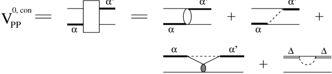
FIG. 3.: Diagrammatic representation of the connected driving term $V^{0,\,con}_{PP}(z)$. The greek letters $\alpha$ and $\alpha^{\prime}$ label either a bare nucleon ${\bar{N}}$ or a $\Delta$.

FIG. 4.: Diagrammatic representation of the $NN$ scattering matrix $T^{X}(z)$ in the presence of a spectator meson.

FIG. 5.: Diagrammatic representation of the dressed $\Delta$ propagator $g_{\Delta}$ (see Eq.  (65)). In order to distinguish $g_{\Delta}$ from the free propagator, it is denoted by a “$\bullet$”.

FIG. 6.: One-boson exchange diagrams for the various interactions involving a ${\bar{N}}\Delta$ configuration. Diagrams (a) through (c) represent retarded contributions (here $\pi$ only). Diagrams (d) through (f) are treated in the energy independent approximation as indicated by the diagrams (d’) through (f’) because of the absence of $\pi N\Delta$ and $\pi\Delta\Delta$ configurations.

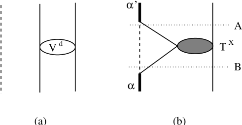
FIG. 7.: Diagrammatic representation of (a) $V^{0}_{XX}$ describing the interaction $V^{d}_{NN}$ between the two nucleons in the ${}^{3}S_{1}$-${}^{3}D_{1}$ channel with a pion as spectator, and (b) of the term $[V_{PX}\,G_{0}(z)\,T^{X}(z)\,G_{0}(z)\,V_{XP}]_{con}$ in Eq. (41).

FIG. 8.: Phase shifts and mixing angle for the ${}^{3}S_{1}$-${}^{3}D_{1}$ channel of $NN$ scattering as a function of the lab kinetic energy $T_{lab}$, compared with the experimental data (solution SM97 of Arndt et al. [31]). Notation of the curves: dotted: separable ansatz (94) with the deuteron wave function of the Bonn OBEPR potential; solid: exact calculation using the full OBEPR potential.

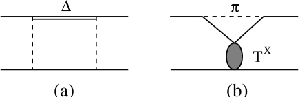
FIG. 9.: Dispersive contributions to the $NN$ interaction: (a) from intermediate $N\Delta$ states, (b) from intermediate offshell $NN$ scattering in the presence of a spectator meson.

FIG. 10.: The renormalization factor $Z^{\pi}_{[2]}(E^{NN}_{p},\,p)$ of Eq. (111) as function of the external nucleon momentum $p$ for different parameter sets: dashed: $\frac{{\left(g^{0}_{\pi}\right)}^{2}}{4\pi}=15$, $\Lambda_{\pi}=500$ MeV; dash-dotted: $\frac{{\left(g^{0}_{\pi}\right)}^{2}}{4\pi}=15$, $\Lambda_{\pi}=1700$ MeV; dotted: $\,\,\frac{\left({g^{0}_{\pi}}\right)^{2}}{4\pi}=25$, $\Lambda_{\pi}=500$ MeV; solid: $\,\,\frac{{\left(g^{0}_{\pi}\right)}^{2}}{4\pi}=25$, $\Lambda_{\pi}=1700$ MeV. A dipole form factor has been used.

FIG. 11.: Phase shift $\delta$ and inelasticity $\rho$ for the ${}^{1}D_{2}$ channel in comparison with experiment (solution SM97 of Arndt et al. [31]) for different retarded potential models (see Table III): full curve: CC(ret$,\pi,\rho,0)$, dotted curve: CC(ret$,\pi,\rho,1)$, and dashed curve: CC(ret$,\pi,\rho,-1)$.

FIG. 12.: Phase shift $\delta$ and inelasticity $\rho$ for the ${}^{3}P_{0}$, ${}^{3}P_{1}$, and ${}^{3}P_{2}$ channels for different retarded potential models as in Fig. 11. Notation of the curves as in Fig. 11 and experimental data: solution SM97 of Arndt et al. [31].

FIG. 13.: Phase shift $\delta$ and inelasticity $\rho$ for the ${}^{1}S_{0}$ , ${}^{3}P_{0}$ and ${}^{3}P_{1}$ channels for different static and retarded approaches: dotted curve: CC$(\mbox{stat1},\pi)$, dashed curve: CC$(\mbox{stat2},\pi)$, dash-dotted curve: CC$(\mbox{stat},\pi,\rho,0)$, and full curve: CC(ret$,\pi,\rho,0)$. The experimental data represent solution SM97 of Arndt et al. [31].

FIG. 14.: Phase shift $\delta$ and inelasticity $\rho$ for the ${}^{1}D_{2}$ and ${}^{3}F_{3}$ channels for different static and retarded approaches as in Fig. 13. Notation of the curves as in Fig. 13 and experimental data: solution SM97 of Arndt et al. [31].

FIG. 15.: Phase shifts, inelasticities and mixing angles for the ${}^{3}P_{2}$-${}^{3}F_{2}$ channel for different static and retarded approaches as in Fig. 13. Notation of the curves as in Fig. 13 and experimental data: solution SM97 of Arndt et al. [31].

FIG. 16.: Diagrammatic representation of the dressed propagator $\widehat{G}_{0}(z)$. The cross represents the one-nucleon counter term $v^{[c]}$.

FIG. 17.: Graphical representation of the scattering amplitude $T^{0,\,con}_{PP}(z)$. The greek letters $\alpha$ and $\alpha^{\prime}$ label either a bare nucleon ${\bar{N}}$ or a $\Delta$. The driving term $V^{0,\,con}_{PP}(z)$ is shown in Fig. 3.

REFERENCES

- [1] C. Herberg et al., Eur. Phys. Journal A 5, 131 (1999); M. Ostrick et al., Phys. Rev. Lett. 83, 276 (1999).
- [2] I. Passchier et al., Phys. Rev. Lett. 82, 4988 (1999).
- [3] H. Arenhövel, G. Kreß, R. Schmidt, and P. Wilhelm, Phys. Lett. B 407, 1 (1997); Nucl. Phys. A 631, 612c (1998).
- [4] R. Machleidt, Adv. Nucl. Phys. Vol. 19, p. 189 (Plenum, New York, 1989)
- [5] J. Carlson and R. Schiavilla, Rev. Mod. Phys. 70, 743 (1998).
- [6] H. Arenhövel and M. Sanzone, Few-Body Syst. Supp. 3, 1 (1991).
- [7] H. Arenhövel, Few-Body Syst. 26, 43 (1999).
- [8] H. Arenhövel, F. Ritz, and Th. Wilbois, Phys. Rev. C 61, 034002 (2000).
- [9] J.M. Laget, Nucl. Phys. A 312, 265 (1978); Can. J. Phys. 62, 1046 (1984).
- [10] M. Schwamb, H. Arenhövel, and P. Wilhelm, Few-Body Syst. 19, 121 (1995).
- [11] H. Tanabe and K. Ohta, Phys. Rev. C 40, 1905 (1989).
- [12] W. Leidemann and H. Arenhövel, Nucl. Phys. A 465, 573 (1987).
- [13] P. Wilhelm and H. Arenhövel, Phys. Lett. B 318, 410 (1993).
- [14] M. Schwamb, H. Arenhövel, P. Wilhelm, and Th. Wilbois, Phys. Lett. B 420 , 255 (1998).
- [15] M. Schwamb, H. Arenhövel, P. Wilhelm, and Th. Wilbois, Nucl. Phys. A 631, 583c (1998).
- [16] M. Schwamb, PhD Thesis, Mainz 1999.
- [17] W.M. Kloet, R.R. Silbar, Nucl. Phys. A 338, 281 (1980); R.R. Silbar, W.M. Kloet, Nucl. Phys. A 338, 317 (1980).
- [18] H. Tanabe, K. Ohta, Nucl. Phys. A 484, 493 (1988).
- [19] W.M. Kloet, R.R. Silbar, Phys. Rev. Lett. 45, 970 (1980).
- [20] Ch. Elster, PhD Thesis, Bonn 1986.
- [21] Ch. Elster, W. Ferchländer, K. Holinde, D. Schütte, and R. Machleidt, Phys. Rev. C 37, 1647 (1988).
- [22] Ch. Elster, K. Holinde, D. Schütte, and R. Machleidt, Phys. Rev. C 38, 1828 (1988).
- [23] A. Bulla and P.U. Sauer, Few-Body Syst. 12, 141 (1992).
- [24] R. Machleidt, K. Holinde, and Ch. Elster, Phys. Rep. 149, 1 (1987).
- [25] P.U. Sauer, Progress in Particle and Nuclear Physics, Vol. 16 , ed. A. Faessler (Pergamon Press, 1986).
-
[26]
H. Pöpping, P.U. Sauer, and X.-Z. Zang,
Nucl. Phys. A 474, 557 (1987);
H. Pöpping, P.U. Sauer, and X.-Z. Zang, Nucl. Phys. A 550, 563 (1992). - [27] M. T. Peña, H. Garcilazo, U. Oelfke, and P. U. Sauer, Phys. Rev. C 45, 1487 (1992).
- [28] P. Wilhelm and H. Arenhövel, Nucl. Phys. A 593, 435 (1995).
- [29] P. Wilhelm and H. Arenhövel, Nucl. Phys. A 609, 469 (1996).
- [30] M. Lacombe, B. Loiseau, J. M. Richard, R. Vinh Mau, J. Côté, P. Pirès, and R. de Tourreil, Phys. Rev. C 21, 861 (1980).
- [31] R.A. Arndt et al., program SAID.
- [32] H. Göller and H. Arenhövel, Few-Body Syst. 13, 117 (1992).
- [33] R.B. Wiringa, R.A. Smith, and T. L. Ainsworth, Phys. Rev. C 29, 1207 (1984).
- [34] V.G.J. Stoks, R.A.M. Klomp, C.P.F. Terheggen, and J.J. de Swart, Phys. Rev. C 49, 2950 (1993).
- [35] A.M. Green and M.E. Sainio, J. Phys. G. 8, 1337 (1982).
- [36] G. Holzwarth and R. Machleidt, Phys. Rev. C 5, 1088 (1997).
- [37] Th. Wilbois, PhD Thesis, Mainz 1996.
- [38] H. Tanabe and K. Ohta, Phys. Rev. C 36, 2495 (1987).
- [39] T.D. Lee, Phys. Rev. 95, 1329 (1954).
- [40] A.N. Kvinikhidze and B. Blankleider, Phys. Rev. C 48, 25 (1993).
- [41] A.N. Kvinikhidze and B. Blankleider, Phys. Lett. B 307, 7 (1993).
- [42] B. Blankleider and A.N. Kvinikhidze, Few-Body Syst. Suppl. 7, 294 (1994).
- [43] P.U. Sauer, M. Sawicki, and S. Furu, Prog. Theor. Phys. 74, 1290 (1985).