Effects of HBT correlations on flow measurements

Abstract

The methods currently used to measure collective flow in nucleus–nucleus collisions assume that the only azimuthal correlations between particles are those arising from their correlation with the reaction plane. However, quantum HBT correlations also produce short range azimuthal correlations between identical particles. This creates apparent azimuthal anisotropies of a few percent when pions are used to estimate the direction of the reaction plane. These should not be misinterpreted as originating from collective flow. In particular, we show that the peculiar behaviour of the directed and elliptic flow of pions observed by NA49 at low $p_{T}$ can be entirely understood in terms of HBT correlations. Such correlations also produce apparent higher Fourier harmonics (of order $n\geq 3$) of the azimuthal distribution, with magnitudes of the order of 1%, which should be looked for in the data.

I Introduction

In a heavy ion collision, the azimuthal distribution of particles with respect to the direction of impact (reaction plane) is not isotropic for non-central collisions. This phenomenon, referred to as collective flow, was first observed fifteen years ago at Bevalac [1], and more recently at the higher AGS [2] and SPS [3] energies. Azimuthal anisotropies are very sensitive to nuclear matter properties [4, 5]. It is therefore important to measure them accurately. Throughout this paper, we use the word “flow” in the restricted meaning of “azimuthal correlation between the directions of outgoing particles and the reaction plane”. We do not consider radial flow [6], which is usually measured for central collisions only.

Flow measurements are done in three steps (see [7] for a recent review of the methods): first, one estimates the direction of the reaction plane event by event from the directions of the outgoing particles; then, one measures the azimuthal distribution of particles with respect to this estimated reaction plane; finally, one corrects this distribution for the statistical error in the reaction plane determination. In performing this analysis, one usually assumes that the only azimuthal correlations between particles result from their correlations with the reaction plane, i.e. from flow This implicit assumption is made, in particular, in the “subevent” method proposed by Danielewicz and Odyniec [8] in order to estimate the error in the reaction plane determination. This method is now used by most, if not all, heavy ion experiments.

However, other sources of azimuthal correlations are known, which do not depend on the orientation of the reaction plane. For instance, there are quantum correlations between identical particles, due to the (anti)symmetry of the wave function : this is the so-called Hanbury-Brown and Twiss effect [9], hereafter denoted by HBT (see [10, 11] for reviews). Azimuthal correlations due to the HBT effect have been studied recently in [12]. In the present paper, we show that if the standard flow analysis is performed, these correlations produce a spurious flow. This effect is important when pions are used to estimated the reaction plane, which is often the case at ultrarelativistic energies, in particular for the NA49 experiment at CERN [13]. We show that when these correlations are properly subtracted, the flow observables are considerably modified at low transverse momentum.

In section 2, we recall how the Fourier coefficients of the azimuthal distribution with respect to the reaction plane are extracted from the two-particle correlation function in the standard flow analysis. Then, in section 3, we apply this procedure to the measured two-particle HBT correlations, and calculate the spurious flow arising from these correlations. Finally, in section 4, we explain how to subtract HBT correlations in the flow analysis, and perform this subtraction on the NA49 data, using the HBT correlations measured by the same experiment. Conclusions are presented in section 5.

II Standard flow analysis

In nucleus–nucleus collisions, the determination of the reaction plane event by event allows in principle to measure the distribution of particles not only in transverse momentum $p_{T}$ and rapidity $y$, but also in azimuth $\phi$, where $\phi$ is the azimuthal angle with respect to the reaction plane. The $\phi$ distribution is conveniently characterized by its Fourier coefficients [14]

$$v_{n}(p_{T},y)\equiv\langle\cos n\phi\rangle={\int_{0}^{2\pi}\cos n\phi{\displaystyle dN\over\displaystyle d^{3}{\bf p}}d\phi\over\int_{0}^{2\pi}{\displaystyle dN\over\displaystyle d^{3}{\bf p}}d\phi}$$ (1)

where the brackets denote an average value over many events. Since the system is symmetric with respect to the reaction plane for spherical nuclei, $\langle\sin n\phi\rangle$ vanishes. Most of the time, because of limited statistics, $v_{n}$ is averaged over $p_{T}$ and/or $y$. The average value of $v_{n}(p_{T},y)$ over a domain ${\cal D}$ of the $(p_{T},y)$ plane, corresponding to a detector, will be denoted by $v_{n}({\cal D})$. In practice, the published data are limited to the $n=1$ (directed flow) and $n=2$ (elliptic flow) coefficients. However, higher harmonics could reveal more detailed features of the $\phi$ distribution [7].

Since the orientation of the reaction plane is not known a priori, $v_{n}$ must be extracted from the azimuthal correlations between the produced particles. We introduce the two-particle distribution, which is generally written as

$${dN\over d^{3}{\bf p_{1}}d^{3}{\bf p_{2}}}={dN\over d^{3}{\bf p_{1}}}{dN\over d^{3}{\bf p_{2}}}\left(1+C({\bf p}_{1},{\bf p}_{2})\right)$$ (2)

where $C({\bf p}_{1},{\bf p}_{2})$ is the two-particle connected correlation function, which vanishes for independent particles. The Fourier coefficients of the relative azimuthal distribution are given by

$$c_{n}(p_{T1},y_{1},p_{T2},y_{2})\equiv\langle\cos n(\phi_{1}-\phi_{2})\rangle={\int\!\!\!\int{\cos n(\phi_{1}-\phi_{2}){\displaystyle dN\over\displaystyle d^{3}{\bf p}_{1}d^{3}{\bf p}_{2}}d\phi_{1}d\phi_{2}}\over\int\!\!\!\int{{\displaystyle dN\over\displaystyle d^{3}{\bf p}_{1}d^{3}{\bf p}_{2}}d\phi_{1}d\phi_{2}}}.$$ (3)

We denote the average value of $c_{n}$ over $(p_{T2},y_{2})$ in the domain ${\cal D}$ by $c_{n}(p_{T1},y_{1},{\cal D})$, and the average over both $(p_{T1},y_{1})$ and $(p_{T2},y_{2})$ by $c_{n}({\cal D},{\cal D})$.

Using the decomposition (2), one can write $c_{n}$ as the sum of two terms:

$$c_{n}(p_{T1},y_{1},p_{T2},y_{2})=c_{n}^{\rm flow}(p_{T1},y_{1},p_{T2},y_{2})+c_{n}^{\rm non-flow}(p_{T1},y_{1},p_{T2},y_{2})$$ (4)

where the first term is due to flow:

$$c_{n}^{\rm flow}(p_{T1},y_{1},p_{T2},y_{2})=v_{n}(p_{T1},y_{1})v_{n}(p_{T2},y_{2})$$ (5)

and the remaining term comes from two-particle correlations:

$$c_{n}^{\rm non-flow}(p_{T1},y_{1},p_{T2},y_{2})={\int\!\!\!\int{\cos n(\phi_{1}-\phi_{2})C({\bf p}_{1},{\bf p}_{2}){\displaystyle dN\over\displaystyle d^{3}{\bf p}_{1}}{\displaystyle dN\over\displaystyle d^{3}{\bf p}_{2}}d\phi_{1}d\phi_{2}}\over\int\!\!\!\int{{\displaystyle dN\over\displaystyle d^{3}{\bf p}_{1}d^{3}{\bf p}_{2}}d\phi_{1}d\phi_{2}}}$$ (6)

In writing Eq.(5), we have used the fact that $\langle\sin n\phi_{1}\rangle=\langle\sin n\phi_{2}\rangle=0$ and neglected the correlation $C({\bf p}_{1},{\bf p}_{2})$ in the denominator.

In the standard flow analysis, non-flow correlations are neglected [7, 8], with a few exceptions: the correlations due to momentum conservation are taken into account at intermediate energies [15], and correlations between photons originating from $\pi^{0}$ decays were considered in [16]. The effect of non-flow correlations on flow observables is considered from a general point of view in [17]. In the remainder of this section, we assume that $c_{n}^{\rm non-flow}=0$. Then, $v_{n}$ can be calculated simply as a function of the measured correlation $c_{n}$ using Eq.(5), as we now show. Note, however, that Eq.(5) is invariant under a global change of sign: $v_{n}(p_{T},y)\to-v_{n}(p_{T},y)$. Hence the sign of $v_{n}$ cannot be determined from $c_{n}$. It is fixed either by physical considerations or by an independent measurement. For instance, NA49 chooses the minus sign for the $v_{1}$ of charged pions, in order to make the $v_{1}$ of protons at forward rapidities come out positive [13]. Averaging Eq.(5) over $(p_{T1},y_{1})$ and $(p_{T2},y_{2})$ in the domain ${\cal D}$, one obtains :

$$v_{n}({\cal D})=\pm\sqrt{c_{n}({\cal D},{\cal D})}.$$ (7)

This equation shows in particular that the average two-particle correlation $c_{n}({\cal D},{\cal D})$ due to flow is positive. Finally, integrating (5) over $(p_{T2},y_{2})$, and using (7), one obtains the expression of $v_{n}$ as a function of $c_{n}$:

$$v_{n}(p_{T1},y_{1})=\pm{c_{n}(p_{T1},y_{1},{\cal D})\over\sqrt{c_{n}({\cal D},{\cal D})}}.$$ (8)

This formula serves as a basis for the standard flow analysis.

Note that the actual experimental procedure is usually different: one first estimates, for a given Fourier harmonic $m$, the azimuth of the reaction plane (modulo $2\pi/m$) by summing over many particles. Then one studies the correlation of another particle (in order to remove autocorrelations) with respect to the estimated reaction plane. One can then measure the coefficient $v_{n}$ with respect to this reaction plane if $n$ is a multiple of $m$. In this paper, we consider only the case $n=m$. Both procedures give the same result, since they start from the same assumption (the only azimuthal correlations are from flow). This equivalence was first pointed out in [18].

III Azimuthal correlations due to the HBT effect

The HBT effect yields two-particle correlations, i.e. a non-zero $C({\bf p}_{1},{\bf p}_{2})$ in Eq.(2). According to Eq.(6), this gives rise to an azimuthal correlation $c_{n}^{\rm non-flow}$, which contributes to the total, measured correlation $c_{n}$ in Eq.(4). In particular, there will be a correlation between randomly chosen subevents when one particle of a HBT pair goes into each subevent. The contribution of HBT correlations to $c_{n}^{\rm non-flow}$ will be denoted by $c_{n}^{\rm HBT}$.

In the following, we shall consider only pions. Since they are bosons, their correlation is positive, i.e. of the same sign as the correlation due to flow. Therefore, if one applies the standard flow analysis to HBT correlations alone, i.e. if one replaces $c_{n}$ by $c_{n}^{\rm HBT}$ in Eq.(8), they yield a spurious flow $v_{n}^{\rm HBT}$, which we calculate in this section.

First, let us estimate its order of magnitude. The HBT effect gives a correlation of order unity between two identical pions with momenta ${\bf p_{1}}$ and ${\bf p_{2}}$ if $|{\bf p_{2}}-{\bf p_{1}}|\lesssim\hbar/R$, where $R$ is a typical HBT radius, corresponding to the size of the interaction region. From now on, we take $\hbar=1$. In practice, $R\sim 4$ fm for a semi–peripheral Pb–Pb collision at 158 GeV per nucleon, so that $1/R\sim 50$ MeV/c is much smaller than the average transverse momentum, which is close to $400$ MeV/c: the HBT effect correlates only pairs with low relative momenta.

In particular, the azimuthal correlation due to the HBT effect is short-ranged : it is significant only if $\phi_{2}-\phi_{1}\lesssim 1/(Rp_{T})\sim 0.1$. This localization in $\phi$ implies a delocalization in $n$ of the Fourier coefficients, which are expected to be roughly constant up to $n\lesssim Rp_{T}\sim 10$, as will be confirmed below.

For small $n$ and $(p_{T1},y_{1})$ in ${\cal D}$, the order of magnitude of $c_{n}^{\rm HBT}(p_{T1},y_{1},{\cal D})$ is the fraction of particles in ${\cal D}$ whose momentum lies in a circle of radius $1/R$ centered at ${\bf p_{1}}$. This fraction is of order $(R^{3}\langle p_{T}\rangle^{2}\langle m_{T}\rangle\Delta y)^{-1}$, where $\langle p_{T}\rangle$ and $\langle m_{T}\rangle$ are typical magnitudes of the transverse momentum and transverse mass ($m_{T}=\sqrt{p_{T}^{2}+m^{2}}$, where $m$ is the mass of the particle), respectively, while $\Delta y$ is the rapidity interval covered by the detector. Using Eq.(7), this gives a spurious flow of order

$$\left|v_{n}^{\rm HBT}({\cal D})\right|\sim\left({1\over R^{3}\langle p_{T}\rangle^{2}\langle m_{T}\rangle\Delta y}\right)^{1/2}.$$ (9)

The effect is therefore larger for the lightest particles, i.e. for pions. Taking $R=4$ fm, $\langle p_{T}\rangle\sim\langle m_{T}\rangle\sim 400$ MeV/c and $\Delta y=2$, one obtains $\left|v_{n}({\cal D})\right|\sim 3$ %, which is of the same order of magnitude as the flow values measured at SPS. It is therefore a priori important to take HBT correlations into account in the flow analysis.

We shall now turn to a more quantitative estimate of $c_{n}^{\rm HBT}$. For this purpose, we use the standard gaussian parametrization of the correlation function (2) between two identical pions[19]:

$$C({\bf p}_{1},{\bf p}_{2})=\lambda e^{-q_{s}^{2}R_{s}^{2}-q_{o}^{2}R_{o}^{2}-q_{L}^{2}R_{L}^{2}}$$ (10)

One chooses a frame boosted along the collision axis in such a way that $p_{1z}+p_{2z}=0$ (“longitudinal comoving system”, denoted by LCMS). In this frame, $q_{L}$, $q_{o}$ and $q_{s}$ denote the projections of ${\bf p}_{2}-{\bf p}_{1}$ along the collision axis, the direction of ${\bf p}_{1}+{\bf p}_{2}$ and the third direction, respectively. The corresponding radii $R_{L}$, $R_{o}$ and $R_{s}$, as well as the parameter $\lambda$ ($0\leq\lambda\leq 1$), depend on ${\bf p}_{1}+{\bf p}_{2}$. We neglect this dependence in the following calculation. Note that the parametrization (10) is valid for central collisions, for which the pion source is azimuthally symmetric. Therefore the azimuthal correlations studied in this section have nothing to do with flow. Note also that we neglect Coulomb correlations, which should be taken into account in a more careful study. We hope that repulsive Coulomb correlations between like-sign pairs will be compensated, at least partially, by attractive correlations between opposite sign pairs.

Since $C({\bf p}_{1},{\bf p}_{2})$ vanishes unless ${\bf p}_{2}$ is very close to ${\bf p}_{1}$, we may replace $dN/d^{3}{\bf p_{2}}$ by $dN/d^{3}{\bf p_{1}}$ in the numerator of Eq.(6), and then integrate over ${\bf p}_{2}$. As we have already said, $q_{s}$, $q_{o}$ and $q_{L}$ are the components of ${\bf p}_{2}-{\bf p}_{1}$ in the LCMS, and one can equivalently integrate over $q_{s}$, $q_{o}$ and $q_{L}$. In this frame, $y_{1}\simeq 0$ and one may also replace $dN/d^{3}{\bf p}_{1}$ by $(1/m_{T1})dN/d^{2}{\bf p_{T}}_{1}dy_{1}$. The resulting formula is boost invariant and can also be used in the laboratory frame.

The relative angle $\phi_{2}-\phi_{1}$ can be expressed as a function of $q_{s}$ and $q_{o}$. If $p_{T1}\gg 1/R$, then to a good approximation

$$\phi_{2}-\phi_{1}\simeq{q_{s}/p_{T1}}.$$ (11)

If $p_{T1}\sim 1/R$, Eq.(11) is no longer valid. We assume that $R_{s}\simeq R_{o}$ and use, instead of (11), the following relation :

$$q_{s}^{2}+q_{o}^{2}=p_{T1}^{2}+p_{T2}^{2}-2p_{T1}p_{T2}\cos(\phi_{2}-\phi_{1}).$$ (12)

To calculate $c_{n}^{\rm HBT}(p_{T1},y_{1},{\cal D})$, we insert Eqs.(10) and (11) in the numerator of (6) and integrate over $(q_{s},q_{o},q_{L})$. The limits on $q_{o}$ and $q_{L}$ are deduced from the limits on $(p_{T2},y_{2})$, using the following relations, valid if $p_{T1}\gg 1/R$ :

$$q_{o} = p_{T2}-p_{T1}$$ (13)

$$q_{L} = m_{T1}(y_{2}-y_{1}).$$ (14)

Since $q_{s}$ is independent of $p_{T2}$ and $y_{2}$ (see Eq.(11)), the integral over $q_{s}$ extends from $-\infty$ to $+\infty$.

Note that values of $q_{o}$ and $q_{L}$ much larger than $1/R$ do not contribute to the correlation (10), so that one can extend the integrals over $q_{o}$ and $q_{L}$ to $\pm\infty$ as soon as the point $(p_{T1},y_{1})$ lies in ${\cal D}$ and is not too close to the boundary of ${\cal D}$. By too close, we mean within an interval $1/R_{o}\sim 50$ MeV/c in $p_{T}$ or $1/(R_{L}m_{T})\sim 0.3$ in $y$. One then obtains after integration

$$c_{n}^{\rm HBT}(p_{T1},y_{1},{\cal D})={\lambda\pi^{3/2}\over R_{s}R_{o}R_{L}}\exp\left(-{n^{2}\over 4p_{T1}^{2}R_{s}^{2}}\right){\displaystyle{1\over m_{T1}}{dN\over d^{2}{\bf p_{T}}_{1}dy_{1}}\over\displaystyle\int_{\cal D}{dN\over d^{2}{\bf p_{T}}_{2}dy_{2}}d^{2}{\bf p_{T}}_{2}dy_{2}}.$$ (15)

At low $p_{T}$, Eq.(11) must be replaced by Eq.(12). Then, one must do the following substitution in Eq.(15) :

$$\exp\left(-{n^{2}\over 4\chi^{2}}\right)\rightarrow{\sqrt{\pi}\over 2}\chi e^{-\chi^{2}/2}\left(I_{n-1\over 2}\left({\chi^{2}\over 2}\right)+I_{n+1\over 2}\left({\chi^{2}\over 2}\right)\right)$$ (16)

where $\chi=R_{s}p_{T}$ and $I_{k}$ is the modified Bessel function of order $k$.

Let us discuss our result (15). First, the correlation depends on $n$ only through the exponential factor, which suppresses $c_{n}^{\rm HBT}$ in the very low $p_{T}$ region $p_{T1}\lesssim n/2R_{s}$. For $n$ smaller than $R_{s}\langle p_{T}\rangle\simeq 10$, the correlation depends weakly on $n$, as discussed above. Neglecting this $n$ dependence, (15) reproduces the order of magnitude (9). To see this, we normalize the particle distribution in ${\cal D}$ in order to get rid of the denominator in (15), and the numerator $(1/m_{T1})(dN/d^{2}{\bf p_{T}}_{1}dy_{1})$ is of order $1/\langle p_{T}\rangle^{2}\langle m_{T}\rangle\Delta y$. However, Eq.(15) is more detailed, and shows in particular that the dependence of the correlation on $p_{T1}$ and $y_{1}$ follows that of the momentum distribution in the LCMS (neglecting the $m_{T}$ and $y$ dependence of HBT radii). This is because the correlation $c_{n}^{\rm HBT}$ is proportional to the number of particles surrounding ${\bf p}_{1}$ in phase space.

Let us now present numerical estimates for a Pb–Pb collision at SPS. We assume for simplicity that the $p_{T}$ and $y$ dependence of the particle distribution factorize, thereby neglecting the observed variation of $\langle p_{T}\rangle$ with rapidity [20]. The rapidity dependence of charged pions can be parametrized by [20]:

$${dN\over dy}=\frac{1}{\sigma\sqrt{2\pi}}\exp\left(-\frac{\left(y-\langle y\rangle\right)^{2}}{2\sigma^{2}}\right)$$ (17)

with $\sigma=1.4$ and $\langle y\rangle=2.9$. The normalized $p_{T}$ distribution is parametrized by

$${dN\over d^{2}{\bf p_{T}}}={e^{m/T}\over 2\pi T(m+T)}\exp\left(-{m_{T}\over T}\right).$$ (18)

with $T\simeq 190$ MeV [20]. This parametrization underestimates the number of low-$p_{T}$ pions. The values of $R_{o}$, $R_{s}$ and $R_{L}$ used in our computations, taking into account that the collisions are semi-peripheral, are respectively 4 fm, 4 fm and 5 fm [22]. The correlation strength $\lambda$ is approximately 0.4 for pions [23].

Finally, we must define the domain ${\cal D}$ in Eq.(15). It is natural to choose different rapidity windows for odd and even harmonics, because odd harmonics have opposite signs in the target and projectile rapidity region, by symmetry, and vanish at mid-rapidity ($\langle y\rangle=2.9$), while even harmonics are symmetric around mid-rapidity. Following the NA49 collaboration [21], we take $4<y<6$ and $0.05<p_{T}<0.6$ GeV/c for odd $n$, and $3.5<y<5$ and $0.05<p_{T}<2$ GeV/c for even $n$. We assume that the particles in ${\cal D}$ are 85% pions [13], half $\pi^{+}$, half $\pi^{-}$. Then, for an identified charged pion (a $\pi^{+}$, say) with $p_{T}=p_{T1}$ and $y=y_{1}$, the right-hand side of Eq.(15) must be multiplied by $0.85\times 0.5$, which is the probability that a particle in ${\cal D}$ be also a $\pi^{+}$.

FIG. 1.: Apparent $|v_{n}^{\rm HBT}|$ from HBT correlations as a function of $p_{T}$ in MeV/c. Top : $n=1$ (solid curve), $n=3$ (long dashes), $n=5$ (short dashes). Bottom : $n=2$ (solid curve), $n=4$ (long dashes), $n=6$ (short dashes). The values are smaller for even $n$ than for odd $n$ because the rapidity intervals chosen to estimate the reaction plane differ.

Substituting the correlation calculated from Eq.(15) in Eq.(8), one obtains the value of the spurious flow $v_{n}^{\rm HBT}(p_{T},y)$ due to the HBT effect. Fig.1 displays $\left|v_{n}^{\rm HBT}\right|$, integrated between $4<y<5$ (as are the NA49 data) as a function of $p_{T}$. As expected, $v_{n}^{\rm HBT}$ depends on the order $n$ only at low $p_{T}$, where it vanishes due to the exponential factor in Eq.(15). HBT correlations, which follow the momentum distribution, also vanish if $p_{T}$ is much larger than the average transverse momentum. Assuming that $1/R_{s}\ll m,T$, we find from Eq.(15) that the correlation is maximum at $p_{T}=p_{T\max}$ where

$$p_{T\max}=\left({2T\over m+T}\right)^{1/4}\sqrt{nm\over 2R_{s}}\simeq 60\sqrt{n}~{}{\rm MeV/c},$$ (19)

which reproduces approximately the maxima in Fig.1.

Although data on higher order harmonics are still unpublished, they were shown at the Quark Matter ’99 conference by the NA45 Collaboration [24] which reports values of $v_{3}$ and $v_{4}$ of the same order as $v_{1}$ and $v_{2}$, respectively, suggesting that most of the effect is due to HBT correlations. Similar results were found with NA49 data [25].

IV Subtraction of HBT correlations

Now that we have evaluated the contribution of HBT correlations to $c_{n}^{\rm non-flow}$, we can subtract this term from the measured correlation (left-hand side of Eq.(4), which will be denoted by $c_{n}^{\rm measured}$ in this section) to isolate the correlation due to flow. Then, the flow $v_{n}$ can be calculated using Eq.(8), replacing in this equation $c_{n}$ by the corrected correlation $c_{n}^{\rm flow}=c_{n}^{\rm measured}-c_{n}^{\rm HBT}$. In this section, we show the result of this modification on the directed and elliptic flow data published by NA49 for pions [13].

The published data do not give directly the two-particle correlation $c_{n}^{\rm measured}$, but rather the measured flow $v_{n}^{\rm measured}$. Since these analyses assume that the correlation factorizes according to Eq.(5), we can reconstruct the measured correlation as a function of the measured $v_{n}$. In particular,

$$c_{n}^{\rm measured}(p_{T1},y_{1},{\cal D})=v_{n}^{\rm measured}(p_{T1},y_{1})v_{n}^{\rm measured}({\cal D}).$$ (20)

We then perform the subtraction of HBT correlations in both the numerator and the denominator of Eq.(8).

The integrated flow values measured by NA49 are $v_{1}^{\rm measured}({\cal D})=-3.0\pm 0.1\%$ and $v_{2}^{\rm measured}({\cal D})=3.0\pm 0.1\%$ [21]. After subtraction of HBT correlations, the coefficients are smaller by some 20% : $v_{1}({\cal D})=-2.5\%$ and $v_{2}({\cal D})=2.6\%$.

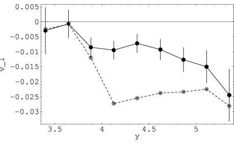
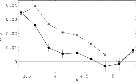
FIG. 2.: Directed flow $v_{1}$ and elliptic flow $v_{2}$ of pions, integrated over $50<p_{T}<350$ MeV/c, as a function of the rapidity, measured by NA49 ($v_{n}^{\rm measured}$, dashed curves) and after subtraction of HBT correlations ($v_{n}$, full curves). For clarity sake, experimental error bars are indicated for the corrected data only.

Fig.2 displays the rapidity dependence of $v_{1}$ and $v_{2}$ at low transverse momentum, where the effect of HBT correlations is largest. Let us first comment on the uncorrected data. We note that $v_{1}^{\rm measured}$ is zero below $y<4$ (i.e. outside ${\cal D}$, where there are no HBT correlations) and jumps to a roughly constant value when $y>4$ (where HBT correlations set in). This gap disappears once HBT correlations are subtracted, and the resulting values of $v_{1}$ are considerably smaller. The values of $v_{2}$ are also much smaller after correction, except near mid-rapidity.

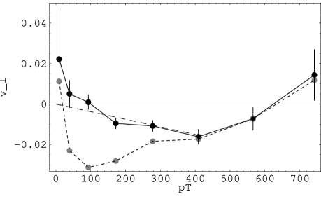
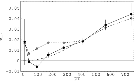
FIG. 3.: Directed flow $v_{1}$ and elliptic flow $v_{2}$ of pions, integrated between $4<y<5$, as a function of the transverse momentum $p_{T}$ in MeV/c, measured by NA49 ($v_{n}^{\rm measured}$, short dashes) and after subtraction of HBT correlations ($v_{n}$, full curves). The long dashes show linear and quadratic fits at low $p_{T}$ for $v_{1}$ and $v_{2}$, respectively.

Fig.3 displays the $p_{T}$ dependence of $v_{1}$ and $v_{2}$. The behaviour of $v_{n}(p_{T})$ is constrained at low $p_{T}$ : if the momentum distribution is regular at ${\bf p_{T}}={\bf 0}$, then $v_{n}(p_{T})$ must vanish like $p_{T}^{n}$. One naturally expects this decrease to occur on a scale of the order of the average $p_{T}$. This is what is observed for protons [13]. However, the uncorrected $v_{1}^{\rm measured}$ and $v_{2}^{\rm measured}$ for pions remain large far below 400 MeV/c. In order to explain this behaviour, one would need to invoke a specific phenomenon occurring at low $p_{T}$. No such phenomenon is known. Even though resonance (mostly $\Delta$) decays are known to populate the low-$p_{T}$ pion spectrum, they are not expected to produce any spectacular increase in the flow.

HBT correlations provide this low-$p_{T}$ scale, since they are important down to $1/R\simeq 50$ MeV/c. Once they are subtracted, the peculiar behaviour of the pion flow at low $p_{T}$ disappears. $v_{1}$ and $v_{2}$ are now compatible with a variation of the type $v_{1}\propto p_{T}$ and $v_{2}\propto p_{T}^{2}$, up to $400$ MeV/c.

V Conclusions

We have shown that the HBT effect produces correlations which can be misinterpreted as flow when pions are used to estimate the reaction plane. This effect is present only for pions, in the $(p_{T},y)$ window used to estimate the reaction plane. Azimuthal correlations due to the HBT effect depend on $p_{T}$ and $y$ like the momentum distribution in the LCMS, i.e. $(1/m_{T})dN/dyd^{2}p_{T}$, and depend weakly on the order of the harmonic $n$.

The pion flow observed by NA49 has peculiar features at low $p_{T}$: the rapidity dependence of $v_{1}$ is irregular, and both $v_{1}$ and $v_{2}$ remain large down to values of $p_{T}$ much smaller than the average transverse momentum, while they should decrease with $p_{T}$ as $p_{T}$ and $p_{T}^{2}$, respectively. All these features disappear once HBT correlations are properly taken into account. Furthermore, we predict that HBT correlations should also produce spurious higher harmonics of the pion azimuthal distribution ($v_{n}$ with $n\geq 3$) at low $p_{T}$, weakly decreasing with $n$, with an average value of the order of 1%. The data on these higher harmonics should be published. This would provide a confirmation of the role played by HBT correlations. More generally, our study shows that although non-flow azimuthal correlations are neglected in most analyses, they may be significant.

Acknowledgements

We thank A. M. Poskanzer and S. A. Voloshin for detailed explanations concerning the NA49 flow analysis and useful comments, and J.-P. Blaizot for careful reading of the manuscript and helpful suggestions.

REFERENCES

- [1] H. Gustafsson et al., Phys. Rev. Lett. 52 (1984) 1590.
- [2] J. Barrette et al., Phys. Rev. Lett. 73 (1994) 2532.
- [3] T. Wienold (NA49 Collaboration) Nucl. Phys. A610 (1996) 76c.
- [4] P. Danielewicz et al., Phys. Rev. Lett. 81 (1998) 2438.
- [5] H. Sorge, Phys. Rev. Lett. 82 (1999) 2048.
- [6] P. Braun-Munzinger, J. Stachel, J. P. Wessels, and N. Xu, Phys. Lett. B344 (1995) 43.
- [7] A. M. Poskanzer and S. A. Voloshin, Phys. Rev. C58 (1998) 1671.
- [8] P. Danielewicz and G. Odyniec, Phys. Lett. 157B (1985) 146.
- [9] R. Hanbury-Brown and R. Q. Twiss, Nature (London) 178 (1956) 1046.
- [10] D. H. Boal, C.-K. Gelbke, and B. K. Jennings, Rev. Mod. Phys. 62 (1990) 553.
- [11] U. A. Wiedemann and U. Heinz, Phys. Rep. 319 (1999) 145.
- [12] S. Mrówczyński, Los Alamos preprint nucl-th/9907099.
-
[13]
H. Appelshäuser et al., NA49 Collaboration,
Phys. Rev. Lett. 80 (1998) 4136.
The data we use in this paper are the revised data available on
the NA49 web page
http://na49info.cern.ch/na49/Archives/Images/Publications/Phys.Rev.Lett.80:4136-4140,1998/ - [14] S. A. Voloshin and Y. Zhang, Z. Phys. C70 (1996) 65.
- [15] P. Danielewicz et al., Phys. Rev. C38 (1988) 120.
- [16] M. M. Aggarwal et al., WA93 Collaboration, Phys. Lett. B403 (1997) 390.
- [17] J.-Y. Ollitrault, Nucl. Phys. A590 (1995) 561c.
- [18] S. Wang et al., Phys. Rev. C44 (1991) 1091.
- [19] G. F. Bertsch, M. Gong, and M. Tohyama, Phys. Rev. C37 (1988) 1896; S. Pratt, T. Csörgő, and J. Zimányi, Phys. Rev. C42 (1990) 2646.
- [20] P. G. Jones (NA49 collaboration), Nucl. Phys. A610 (1996) 188c.
- [21] A. M. Poskanzer, private communication.
- [22] R. Ganz (NA49 collaboration), Los Alamos preprint nucl-ex/9909003, to be published in the Proceedings of Quark Matter’99.
- [23] P. Seyboth for the NA49 Collaboration, NA49 Note number 177 “Pion-Pion correlations in 158 AGeV Pb–Pb collisions from the NA49 experiment”, in the Proceedings of the International Workshop on Multiparticle Production, Correlations and Fluctuations, Matrahaza, Hungary (14-21/6/98).
- [24] B. Lenkeit for the NA45 collaboration, Los Alamos preprint nucl-ex/9910015, to be published in the Proceedings of Quark Matter’99.
- [25] A. M. Poskanzer and S. A. Voloshin, unpublished.