An Isobaric Model for Kaon photoproduction

Abstract

The kaon photoproduction is analyzed up to $E_{\gamma}^{\rm Lab}$=2.0 GeV by using an isobaric model based on effective Lagrangians and by taking a cross symmetry into account. Both pseudovector and pseudoscalar couplings for kaon-baryon-baryon (baryon spin=1/2) interactions are considered with form factors. A vector meson($K^{*}(890)$), an axial vector meson($K_{1}(1270)$), nucleon resonances($J\leq 5/2$), and hyperon resonances($J\leq 3/2$) are treated as participating particles. By determining unknown coupling constants through a systematic fitting of the differential cross section, the total cross section, the single polarization observable, and the radiative kaon capture branching ratio to their experimental data, we find out a simple model which reproduces all the experimental data well.

I Introduction

It is believed that quantum chromodynamics(QCD) is a basic theory of the strong interaction. The QCD was born by combining the Yang and Mills’s non-Abelian gauge theory with the quark model. It has a $SU_{L}(N_{f})\otimes SU_{R}(N_{f})$ symmetry($N_{f}$ is the flavor number) in a massless limit of quark and has a non-perturbative property in the intermediate energy region. In the non-perturbative vacuum, the $SU_{L}(N_{f})\otimes SU_{R}(N_{f})$ symmetry is spontaneously broken down to $SU_{V}(N_{f})$, and the massless Goldstone bosons, which are pseudoscalar mesons with spin and parity $J^{P}=0^{-}$, appear. Because of the non-perturbative property of QCD in the intermediate energy region, we can not obtain sufficient information about nuclear force by directly tackling the QCD. Therefore, in the region, we investigate the nuclear physics by an effective theory which have the basic symmetry in QCD. Since the pseudoscalar meson plays important roles in the intermediate energy nuclear physics using such effective theory, understanding the property of the pseudoscalar meson is an inevitable study in the nuclear physics at the energy region. In specific, photo- and electro-production of pseudoscalar mesons is complementary to the reaction, such as the electron-nucleus scattering, $\pi$-nucleus scattering, muon capture, and radiative pseudoscalar meson capture. Compared with the pseudoscalar meson, the real or virtual photon, as a probing particle, is very weakly absorbed in the nucleus. Therefore, the photo- or electro-production of pseudoscalar meson gives more cleaner and more reliable information on the property of pseudoscalar meson interactions with nuclei than the hadron-induced reactions.

On the other hand, with increasing interests in hypernuclei, the kaon electromagnetic productions on nuclei have been interested as the reaction for producing the hypernuclei. The study of kaon photoproduction (KP) on a nucleon started in the late 50’s, but a comprehensive description of the underlying reaction mechanism is still not available because copious number of nucleonic and hyperonic resonances may intervene in the process due to the high threshold energy($E_{\gamma}^{\rm Lab}=910$MeV ) of the reaction even near threshold. Moreover, most of the relevant coupling constants are still unknown.

However, with the advance of high energy and high duty cycle electron accelerators and detectors at the Thomas Jefferson National Accelerator Facility(TJNAF), ELectron Stretcher Accelerator (ELSA) and European Synchrotron Radiation Facility(USRF), the high-current and polarized beams in the energy domain of a few GeV’s are provided. Consequently, the sufficient and high-precision experimental data of kaon photo- and electro-production are available now or will be in the near future. Therefore, it is an urgent task to establish and to improve the theoretical models about the kaon photo(electro)production.

Most theoretical studies for KP, so far, have been performed by using dispersion relations[1]-[2], multipole analysis[3], quark-based models[4]-[6], and isobaric models[7]-[22]. In the dispersion theory or multipole analysis, amplitudes are obtained in K-$\Lambda$ center of mass (c.m.) reference frame, so that transforming them into other frames is cumbersome and ambiguous. In addition, it is difficult to discuss non-local and off-shell effects, which turned out to play a significant role in nuclear applications of the elementary KP amplitudes. Moreover, in the dispersion theory, due to a high-energy threshold of the reaction, the multi-pion channels $\gamma+N\rightarrow N+m\pi$ with $m$=1 to 4 are already open for $K^{+}\Lambda$ process. The inclusion of these reactions leads to very complicated integral equations among the partial amplitudes. To solve the integral equations, unjustifiable approximations are needed. Advantage of using a quark-based model is to describe the reaction by an unified scheme and to explain the reaction well with relatively less parameters than other models. But nuclear application of the model is also not easy.

Finally, the isobaric models are widely used methods to investigate the KP between threshold and roughly $E_{\gamma}^{\rm Lab}=2.0$ GeV region. Based on pioneer works of Thom[8] in 1960’s and Renard and Renard [9] in 1970’s, Hsiao and Cotanch [23] and Adelseck, Bennhold, and Wright[10] revived the models in 1980’s.

All these formulas use the Feynman diagrammatic technique where vertex functions are obtained from a relevant effective Lagrangian. As well known, there are two coupling types of kaon and baryons with $J=\frac{1}{2}$ in strong vertex. One is a pseudoscalar(PS) coupling where a kaon-nucleon-hyperon ($KNY$) vertex is described by $g_{KNY}\gamma_{5}$ with a PS coupling constant of $KNY$, $g_{KNY}$, and the other is a pseudovector(PV) coupling in which the $KNY$ vertex is described by $\frac{f_{KNY}}{M_{N}+M_{Y}}q\!\!\!/\gamma_{5}$, where $f_{KNY}$, $M_{N},\ M_{Y}$, and $q$ are a PV-coupling constant, a nucleon mass, a hyperon mass, and an outgoing kaon four-momentum, respectively.

Through a chiral rotation[24], the nonlinear $\sigma$ model, in which $\pi NN$ coupling is PV type, is related to the linear sigma model adopting PS coupling. In an infinite sigma mass limit, both models give identical results. But it is valid only at a tree order because the nonlinear version encounters divergences in one or more loops calculations, so that one can not confirm the equivalence between two coupling schemes as far as one includes higher order terms as an effective interaction under a tree order.

In kaon(or pion) photoproduction, without the Pauli-type electromagnetic interactions stemming from meson loop(s) i.e. higher order terms, two coupling schemes give the same predictions [25]. Since the Pauli interaction gives large contribution it is unavoidable to consider the interaction in the tree approximation calculation. The two coupling schemes, consequently, give different predictions.

In case of a charged pion photoproduction, the deviation from both coupling schemes turned out to be small enough to neglect, because the Kroll-Rudermann term in PV scheme, which is also included in the nucleon pole term in PS scheme, is dominant at the threshold. For a neutral pion production, the deviation is significant [26] because the Kroll-Rudermann term disappears in the PV description. The PS coupling description overestimates the experimental ${E_{0+}}$ amplitude at the threshold about factor 10 even taking the neutral vector mesons’ contributions into account, while the PV scheme, at the threshold, satisfies a conventional low energy theorem(LET)[27]. That is the reason why the PV scheme has been preferred to the PS coupling in describing the pion photoproduction near threshold. Although recent experiments [30, 50] and many theoretical researches[31, 32, 33, 34] about $E_{0+}$ show that the LET disagreed to experimental values more or less, the superior prediction of PV Born terms to that of PS Born terms remains true at the threshold. Beyond threshold two descriptions yield nearly identical predictions [35] because the contribution from $\Delta(1232)$ dominates over that of other spin $\frac{1}{2}$ baryons.

In the KP, it is not still clear which is better of the two coupling schemes. Moreover, the contributions of the spin $\frac{1}{2}$ particles are comparable to those of particles with other spins. Therefore, the difference between the PV and PS coupling schemes in this reaction is expected to be much larger than in the pion photoproduction.

Nevertheless, until now, most calculations based on an isobaric model were carried out by the PS coupling scheme. Some works[11, 21, 36] were done by using the PV coupling, but they used models oversimplified. Namely, Bennhold et al. [11] tried to fit phenomenologically the available data for $\gamma+p\rightarrow K^{+}+\Lambda$ by using the model of Adelseck et al.[10] without $K_{1}$ axial vector meson, and obtained very different sets of coupling constants for the two coupling schemes. Feuster et al. [36], by using a unitary model, investigated photon- and meson-induced reactions. In their calculation only nucleon resonances with $J\leq\frac{3}{2}$ were considered with strong form factors in a gauge invariant way by using the Haberzettl’s and Ohta’s gauge prescriptions explained in Section IV. In the paper, they studied the difference between the PV- and PS-coupling schemes and between the two gauge prescriptions. However, they didn’t consider some important contributions : Firstly, the spin $\frac{5}{2}$ particle was excluded in their calculation. It was shown to play an important role in reproducing the polarization data in Ref. [19, 20]. Secondly, they didn’t take the contribution from hyperon resonances into account. Their contributions play a vital role in this reaction. For example, in the previous works for the radiative kaon capture[37, 38, 39, 41, 42], it was founded that $\Lambda(1405)$ gave a dominant contribution to the reaction. Since the radiative kaon capture and the KP are related to each other by a crossing symmetry they should be simultaneously parameterized. Therefore, in the more extended model spaces, the more extensive study using the PV-coupling scheme and scrupulous comparison for both coupling schemes are needed.

One of main goal of this paper is to construct the pseudovector model to reproduce well all of existing experiment data of the reaction and the radiative kaon capture up to $2.1$ GeV of the photon energy by using a $SU(3)$ symmetry and nonrelativistic quark model(NRQM), and to compare the PV-model and the PS-model, and to investigate the effect of off shell strong form factor in the reaction.

In the study up to 2.1 GeV of photon energy, we adopt an isobaric model based on the effective Lagrangian method and consider a $K^{*}$ vector meson and a $K_{1}$ axial vector meson as exchanged resonance particles in $t-$channel, the nucleon resonances with spin($J\leq$ $\frac{5}{2}$) in $s-$channel, and the hyperon resonances with spin($J\leq$ $\frac{3}{2}$) in $u-$channel. The unknown parameters are determined by a fitting procedure, which is carried out by imposing the constraint conditions from about 20 $\%$ broken $SU(3)$ symmetry and the NRQM[46, 47] for strong and electro-magnetic decay widths of resonances. As for couplings, pseudovector (PV) coupling Lagrangians and pseudoscalar (PS) Lagrangians are used for their mutual comparison.

Since the hadron is treated as a point particle, effect of the internal structure of the hadron is not considered in the effective Lagrangian approach. It causes a divergent behavior of the reaction amplitude as increasing an incident photon energy. Therefore, we introduce the form factor in the strong vertex. However, it spoils a gauge invariance because the strong form factor is inserted into the vertex by hand. The hadronic form factor is, thus, introduced in a gauge invariant manner by using Haberzettl’s and Ohta’s prescriptions and dependence of this reaction on the gauge prescriptions is examined in our model. This reaction is also studied without the strong form factors for the comparison with the case form factor used.

This paper is constructed as the following order. In Section II, with a simple explanation of kinematics and invariant amplitude used through this paper, definitions of the physical observables such as differential cross section, single polarization observables, and radiative capture are given. In Section III, interaction Lagrangians and invariant amplitudes for each PV- and PS-coupling schemes are presented. The form factors and gauge prescriptions are described in Section IV. In Section V, we discuss our fitting strategy to determine the coupling constants and to select the particle included in our model. In Section VI, our results and discussions are given. Finally, conclusions are presented in Section VII.

II Basic Formalism

A Kinematics

In this section, we present kinematical relations among kinetic variables and an invariant amplitude of the kaon photoproduction:

$$\gamma(k)+N(p)\longrightarrow K^{+}(q)+\Lambda(p^{\prime})~{},$$ (1)

where $p$, $k$, $p^{\prime}$ and $q$ are momenta of nucleon(N), photon$(\gamma)$, $\Lambda$, and kaon($K^{+}$), respectively. The Mandelstam variables are given below

$$s=(p+k)^{2}=(q+p^{\prime})^{2},~{}u=(q-p)^{2}=(k-p^{\prime})^{2},~{}t=(k-q)^{2}=(p^{\prime}-p)^{2}$$ (2)

with a well-known relation $s+u+t=M^{2}+M_{\Lambda}^{2}+m_{K}^{2}$, where $M$, $m_{K}$, and $M_{\Lambda}$ are the masses of $N$, $K^{+}$, and $\Lambda$, respectively.

As depicted in Fig. 1, we choose the $+z$-axis along the incident photon direction and $\theta$ as the production angle between the photon and the kaon. The momenta of the initial and the final particles are thus expressed in the c.m. as

$$k^{\mu} = (k^{*},\ 0,\ 0,\ k^{*}),p^{\mu}=(E,\ 0,\ 0,\ -k^{*})~{},~{}$$ (3)

$$q^{\mu} = (\omega,\ q^{*}\cos\theta,\ 0,\ q^{*}\sin\theta)~{},~{}p^{\prime\mu}=(E^{\prime},\ -q^{*}\cos\theta,\ 0,\ -q^{*}\sin\theta)~{},$$ (4)

where $k^{*}$ and $q^{*}$ are the magnitude in the c.m. system given in terms of photon lab. energy $k_{lab}$

$$k^{*}=\frac{M}{W}k_{lab}~{},~{}q^{*}=\frac{\sqrt{(s-M^{2}-m_{K}^{2})^{2}-4m_{K}^{2}M^{2}}}{2W}~{},$$ (5)

where $W=\sqrt{s}$.

The ${\cal S}$-matrix is expressed as follows

$${\cal S}_{fi}=\frac{1}{(2\pi)^{2}}\delta^{4}(p+k-p^{\prime}-q)\left[\frac{M_{p}M_{\Lambda}}{4E_{\Lambda}E_{p}E_{\gamma}E_{K}}\right]^{1/2}{\cal M}_{fi}~{}.$$ (6)

To keep the gauge invariance of ${\cal M}_{fi}$ the following self gauge invariant operators ${\cal O}_{j}$ have been used [10]

$${\cal O}_{1} = \frac{1}{2}\gamma_{5}[k\!\!\!/,\epsilon\!\!\!/],$$ (7)

$${\cal O}_{2} = 2\gamma_{5}(\epsilon\cdot pk\cdot p^{\prime}-\epsilon\cdot p^{\prime}k\cdot p),$$ (8)

$${\cal O}_{3} = \gamma_{5}(\epsilon\!\!\!/k\cdot p-k\!\!\!/\epsilon\cdot p),$$ (9)

$${\cal O}_{4} = \gamma_{5}(\epsilon\!\!\!/k\cdot p^{\prime}-k\!\!\!/\epsilon\cdot p^{\prime}).$$ (10)

The ${\cal M}_{fi}$ is expanded, in terms of ${\cal O}_{j}$, as

$${\cal M}_{fi}=\bar{u}_{\Lambda}(p^{\prime},s^{\prime})\sum_{j=1}^{4}{\cal A}_{j}{\cal O}_{j}u_{N}(p,s)~{},$$ (11)

where $u_{N}(p,s)$ and $\bar{u}_{\Lambda}(p^{\prime},s^{\prime})$ are Dirac-spinors of proton and lambda and $s$ and $s^{\prime}$ represent their spin states. We write also ${\cal M}_{fi}$ in terms of Chew, Goldberger, Low, and Nambu(CGLN) amplitudes ${\cal F}_{i}$[48]

$${\cal M}_{fi}^{\lambda}=\biggl{(}\frac{\sqrt{M_{\Lambda}M}}{4\pi W}\biggr{)}^{-1}\chi_{f}^{\dagger}{\cal F}^{\lambda}\chi_{i}~{},$$ (12)

with

$${\cal F}^{\lambda}={\cal F}_{1}\vec{\sigma}\cdot\vec{\epsilon}^{\lambda}+{\cal F}_{2}i\vec{\sigma}\cdot\hat{q}\vec{\sigma}\cdot(\hat{\epsilon}^{\lambda}\times\hat{k})+{\cal F}_{3}\vec{\sigma}\cdot\hat{k}\hat{q}\cdot\hat{\epsilon}^{\lambda}+{\cal F}_{4}\vec{\sigma}\cdot\hat{q}\vec{\epsilon}^{\lambda}\cdot\hat{q}~{},$$ (13)

where $\lambda$ represents a polarization state of the photon. In connection with the ${\cal A}_{i}$, the ${\cal F}_{j}$ are given by

$${\cal F}_{1} = \frac{|\vec{k}|}{4\pi}\sqrt{\frac{E_{\Lambda}+M_{\Lambda}}{2W}}\left[{\cal A}_{1}-\frac{W+M}{2}{\cal A}_{3}-\frac{k.p^{\prime}}{W-M}{\cal A}_{4}\right],$$ (14)

$${\cal F}_{2} = -\frac{|\vec{k}|}{4\pi}\sqrt{\frac{E_{\Lambda}-M_{\Lambda}}{2W}}\left[{\cal A}_{1}+\frac{W-M}{2}{\cal A}_{3}+\frac{k.p^{\prime}}{W+M}{\cal A}_{4}\right],$$ (15)

$${\cal F}_{3} = -\frac{|\vec{k}||\vec{q}|}{4\pi}\sqrt{\frac{E_{\Lambda}+M_{\Lambda}}{2W}}\left[(W-M){\cal A}_{2}-{\cal A}_{4}\right],$$ (16)

$${\cal F}_{4} = \frac{|\vec{k}|}{4\pi}\sqrt{\frac{E_{\Lambda}-M_{\Lambda}}{2W}}\left[(W+M){\cal A}_{2}+{\cal A}_{4}\right]~{}.$$ (17)

B Differential Cross Section and Single Polarization Observables

Using the ${\cal M}_{fi}^{\lambda}$ in Eq.(12) we can write a differential cross section in the c.m. frame of $K-\Lambda$ as follows

$$\left(\frac{d\sigma}{d\Omega}\right)_{\mbox{c.m.}}=\frac{1}{4}\sum_{s_{i},s_{f},\lambda}\frac{q^{*}}{k^{*}}\left|\frac{\sqrt{M_{\Lambda}M_{p}}}{4\pi W}{\cal M}_{fi}^{\lambda}\right|^{2}.$$ (18)

The $\Lambda$-polarization asymmetry($P$), beam polarization symmetry($\Sigma$), and target-polarization asymmetry($T$) are defined by[14]

$$P = \frac{(d\sigma/d\Omega)^{(+)}-(d\sigma/d\Omega)^{(-)}}{(d\sigma/d\Omega)^{(+)}+(d\sigma/d\Omega)^{(-)}},$$ (19)

$$\Sigma = \frac{(d\sigma/d\Omega)^{(+)}-(d\sigma/d\Omega)^{(-)}}{(d\sigma/d\Omega)^{(+)}+(d\sigma/d\Omega)^{(-)}},$$ (20)

$$T = \frac{(d\sigma/d\Omega)^{(\perp)}-(d\sigma/d\Omega)^{(\parallel)}}{(d\sigma/d\Omega)^{(\perp)}+(d\sigma/d\Omega)^{(\parallel)}}~{},$$ (21)

where +(–) represents that a proton(for $T$) or a lambda(for $P$) is polarized parallel(antiparallel) to the direction($\frac{\vec{k}^{*}\times\vec{q}^{*}}{|\vec{k}^{*}\times\vec{q}^{*}|}$). $\perp(\parallel)$ denotes that the photon is linearly polarized perpendicular(parallel) to the reaction plane.

C Branching Ratio of Radiative Kaon Capture

The KP is restricted by a crossing symmetry [54]: The matrix element for a process containing an antiparticle of 4-momentum $p_{\mu}$ in the initial (final) state is identical with the matrix element for the ”crossed” process , which contains the corresponding particle of 4-momentum $-p_{\mu}$ in the final (initial) state. The ”crossed” process of KP is the radiative kaon capture(RKC). Therefore, we can easily obtain the RKC amplitude, ${\cal M}_{rad}$, from the KP amplitude, ${\cal M}_{pho}$, as follows

$${\cal M}_{rad} \equiv {\cal M}_{K^{-}(q)+p(p)\longrightarrow\gamma(k)+\Lambda(p^{\prime})},$$ (22)

$$= {\cal M}_{pho}\equiv{\cal M}_{\gamma(-k)+p(p)\longrightarrow K^{+}(-q)+\Lambda(p^{\prime})}~{},$$ (23)

from which we get the following changing rules among the Mandelstam variables

$${\rm rad.\ cap.}\ \ \ \ \ \ \ \ \ {\rm pho.\ kaon}$$ (24)

$$s = (p+q)^{2}\longrightarrow(p-q)^{2}=u,$$ (25)

$$u = (p-k)^{2}\longrightarrow(p+k)^{2}=s,$$ (26)

$$t = (k-q)^{2}\longrightarrow(q-k)^{2}=t.$$ (27)

Therefore, the amplitude ${\cal M}_{rad}$ is given by[55]

$${\cal M}_{rad}(s,u,t)={\cal M}_{pho}(u,s,t).$$ (28)

The only available data for the radiative kaon capture is a branching ratio which is defined by

$$R_{\gamma\Lambda}=\frac{\Gamma(K^{-}p\rightarrow\gamma\Lambda)}{\Gamma(K^{-}p\rightarrow\rm{all})}.$$ (29)

In a kaonic hydrogen atom, the kaon, whose momentum is approximately zero, is strongly captured from an S-state. Since a range of strong interaction is very short the kaon wave function is approximated as the value evaluated at the proton i.e. $\phi_{K}(0)$. The decay rate for the process is thus given by

$$\Gamma_{K^{-}p\rightarrow\Lambda\gamma}=|\phi_{K}(0)|^{2}\frac{M_{\Lambda}k}{4\pi(m_{K}+M)m_{K}}\frac{1}{2}\sum_{{\rm\lambda,s_{\Lambda},s_{p}}}|{\cal M}_{rad}|^{2}~{},$$ (30)

where $\lambda,\ s_{\Lambda}$, and $s_{p}$ are a photon polarization, a $\Lambda$ spin, and a proton spin, respectively. The total rate for all $K^{-}p$ processes is

$$\Gamma_{K^{-}p\rightarrow{\rm all}}=2W_{p}|\phi_{K}(0)|^{2}~{},$$ (31)

where $W_{p}$ is an imaginary part of the $K^{-}p$ pseudopotential and uses a value[39] $560\pm 135$MeV fm³. By using Eqs. (30) and (31) we obtain the following branching ratio of this process

$$R_{\gamma\Lambda}=\frac{M_{\Lambda}E_{\gamma}}{8\pi W_{p}(m_{K}+M)m_{K}}\frac{1}{2}\sum_{{\rm\lambda,s_{\Lambda},s_{p}}}|{\cal M}_{rad}|^{2}.$$ (32)

III Interaction Lagrangians and Invariant Amplitudes

Under a tree approximation, the KP amplitudes on a proton are obtained from the Feynman diagrams in Fig. 2. For convenience, we explicitly write down each reaction matrix ${\cal M}$ corresponding to each intermediate particle in Born terms, vector meson terms, nucleon resonance terms($N^{*}$), and hyperon resonance terms($Y^{*}$) listed in Table I. The total reaction matrix is thus obtained as a sum of all terms mentioned above:

$${\cal M}={\cal M}(Born)+\sum_{B=N^{*},Y^{*},K^{*},K_{1}}{\cal M}(B).$$ (33)

For more compact forms of Lagrangians, the following isospinors for $K,K^{*},K_{1}$ are used

$$K=\left(\begin{array}[]{c}K^{+}\\ K^{0}\end{array}\right)$$ (34)

$$\begin{array}[]{cc}K^{*}=\left(\begin{array}[]{c}K^{*+}\\ K^{*0}\end{array}\right),&\;\;\;\;\par K_{1}=\left(\begin{array}[]{c}K_{1}^{+}\\ K_{1}^{0}\end{array}\right)~{}.\end{array}$$ (35)

For nucleon($N$) and nucleon resonances ($N^{*}$) we also write the isospinors

$$\begin{array}[]{cc}N=\left(\begin{array}[]{c}p\\ n\end{array}\right),&\;\;\;\;N^{*}=\left(\begin{array}[]{c}N^{*+}\\ N^{*0}\end{array}\right)\end{array}$$ (36)

and those for isovector $\vec{\Sigma}$ and its resonance $\vec{\Sigma}^{*}$ are given by

$$\begin{array}[]{cc}\vec{\Sigma}=\left(\begin{array}[]{c}\Sigma^{+}\\ \Sigma^{0}\\ \Sigma^{-}\end{array}\right),&\;\;\;\;\vec{\Sigma}^{*}=\left(\begin{array}[]{c}\Sigma^{*+}\\ \Sigma^{*0}\\ \Sigma^{*-}\end{array}\right).\end{array}$$ (37)

A Born Terms

Electromagnetic interaction Lagrangians for Born terms are given as

$${\cal L}_{\gamma NN} = -e\bar{N}\left\{\frac{1}{2}(1+\tau_{3})A\!\!\!/+\frac{1}{2}((\kappa_{p}+\kappa_{n})+(\kappa_{p}-\kappa_{n})\tau_{3})\frac{F^{\mu\nu}}{4M}\sigma_{\mu\nu}\right\}N,$$ (38)

$${\cal L}_{\gamma\Lambda\Lambda} = -e\kappa_{\Lambda}\frac{F^{\mu\nu}}{4M}\bar{\Lambda}\sigma_{\mu\nu}\Lambda,$$ (39)

$${\cal L}_{\gamma\Lambda\Sigma} = -e\kappa(\Sigma\Lambda)\left\{\frac{F^{\mu\nu}}{4M}(\bar{\Sigma}^{3}\sigma_{\mu\nu}\Lambda+\bar{\Lambda}\sigma_{\mu\nu}\Sigma^{3})\right\},$$ (40)

$${\cal L}_{\gamma KK} = ie(\partial_{\mu}K^{+}K^{-}-\partial_{\mu}K^{-}K^{+})A^{\mu},$$ (41)

where $e$ is a charge of proton, $\kappa_{p}$, $\kappa_{n}$, and $\kappa_{\Lambda}$ are, respectively, the anomalous magnetic moment of a proton, a neutron, and $\Lambda$. The $\kappa(\Sigma\Lambda)$ is a $\Sigma^{0}\Lambda$-transition magnetic moment. Photon field strength is given as

$$F_{\mu\nu}=(\partial_{\mu}A_{\nu}-\partial_{\nu}A_{\mu}),$$ (42)

and charged eigen-kaon fields $K^{\pm}$ are defined by

$$K^{\pm}=\frac{1}{\sqrt{2}}(K^{1}\pm iK^{2})~{}.$$ (43)

Lagrangians in strong interactions are constructed by two coupling schemes, PV and PS, which are expressed as

$${\cal L}_{KN\Lambda}^{PV} = \frac{f_{KN\Lambda}}{m_{K}}(\partial^{\mu}K^{\dagger}\bar{\Lambda}\gamma_{\mu}\gamma_{5}N+\bar{N}\gamma_{\mu}\gamma_{5}\Lambda\partial^{\mu}K),$$ (44)

$${\cal L}_{KN\Sigma}^{PV} = \frac{f_{KN\Sigma}}{m_{K}}(\partial^{\mu}K^{\dagger}\bar{\vec{\Sigma}}\cdot\vec{\tau}\gamma_{\mu}\gamma_{5}N+\bar{N}\gamma_{\mu}\gamma_{5}\bm{\tau}\cdot\vec{\Sigma}\partial^{\mu}K),$$ (45)

$${\cal L}_{KN\Lambda}^{PS} = -ig_{KN\Lambda}(\bar{\Lambda}\gamma_{5}N+\bar{N}\gamma_{5}\Lambda)K,$$ (46)

$${\cal L}_{KN\Sigma}^{PS} = -ig_{KN\Sigma}(K^{\dagger}\bar{\vec{\Sigma}}\cdot\vec{\tau}\gamma_{5}N+\bar{N}\gamma_{5}\bm{\tau}\cdot\vec{\Sigma}K),$$ (47)

where $m_{K}$ is a kaon mass, and $f_{KN\Lambda}$, $f_{KN\Sigma}$, $g_{KN\Lambda}$, and $g_{KN\Sigma}$ are PV and PS coupling constants, respectively.

Using the vertex factor and the propagator calculated from the above Lagrangians, the Born amplitudes for the PV coupling scheme are written as

$${\cal M}_{s}^{PV} = {\cal M}_{s}^{PS}+e\frac{g_{{}_{KN\Lambda}}}{M+M_{\Lambda}}\bar{u}_{\Lambda}\gamma_{5}\left(\epsilon\!\!/+\mu_{p}\frac{1}{2}[k\!\!\!/,\epsilon\!\!/]\right)u,$$ (48)

$${\cal M}_{u(\Lambda)}^{PV} = {\cal M}_{u(\Lambda)}^{PS}+e\mu_{\Lambda}\frac{g_{{}_{KN\Lambda}}}{M+M_{\Lambda}}\bar{u}_{\Lambda}\frac{1}{2}[k\!\!\!/,\epsilon\!\!/]\gamma_{5}u,$$ (49)

$${\cal M}_{u(\Sigma)}^{PV} = {\cal M}_{u(\Sigma)}^{PS}+e\mu(\Sigma\Lambda)\frac{g_{{}_{KN\Sigma}}}{M+M_{\Sigma}}\bar{u}_{\Lambda}\frac{1}{2}[k\!\!\!/,\epsilon\!\!/]\gamma_{5}u,$$ (50)

$${\cal M}_{KR}^{PV} = -e\frac{g_{{}_{KN\Lambda}}}{m_{K}}\bar{u}_{\Lambda}\gamma_{5}\epsilon\!\!/u,$$ (51)

$${\cal M}_{t}^{PV} = {\cal M}_{t}^{PS}=eg_{{}_{KN\Lambda}}\bar{u}_{\Lambda}\gamma_{5}u\frac{\epsilon\cdot(2q-k)}{t-m_{K}^{2}}~{},$$ (52)

where $\mu_{B}={{\kappa_{B}}\over{2M}}$ for $B=p,\Lambda,(\Sigma\Lambda)$ and subscripts $s,\ u$ and $t$ refer to $s-,\ u-$ and $t-$channel (diagrams (a)-(c) in Fig. 2), respectively. The ${\cal M}_{KR}^{PV}$ is an amplitude corresponding to the diagram (d) in Fig. 2. The PS coupling versions are given by

$${\cal M}_{s}^{PS} = eg_{{}_{KN\Lambda}}\bar{u}_{\Lambda}\gamma_{5}\,\frac{p\!\!\!/+k\!\!\!/+M}{s-M^{2}}\left(\epsilon\!\!/+\mu_{p}\frac{1}{2}[k\!\!\!/,\epsilon\!\!/]\right)u,$$ (53)

$${\cal M}_{u(\Lambda)}^{PS} = e\mu_{\Lambda}g_{{}_{KN\Lambda}}\bar{u}_{\Lambda}\frac{1}{2}[k\!\!\!/,\epsilon\!\!/]\frac{p\!\!\!/-q\!\!\!/+M_{\Lambda}}{u-M_{\Lambda}^{2}}\gamma_{5}u,$$ (54)

$${\cal M}_{u(\Sigma)}^{PS} = e\mu(\Sigma\Lambda)g_{{}_{KN\Sigma}}\bar{u}_{\Lambda}\frac{1}{2}[k\!\!\!/,\epsilon\!\!/]\,\frac{p\!\!\!/-q\!\!\!/+M_{\Sigma}}{u-M_{\Sigma}^{2}}\gamma_{5}u~{},$$ (55)

with a relation $g_{{}_{KN\Lambda(\Sigma)}}=f_{{}_{KN\Lambda(\Sigma)}}\frac{M+M_{\Lambda(\Sigma)}}{m_{K}}$.

B Spin 1 Mesons

For the $K^{*}(890)(J^{P}=1^{-})$, the following Lagrangians are used

$${\cal L}_{K^{*}N\Lambda} = \bar{\Lambda}\left\{\biggl{(}G_{\rm v}\gamma_{\mu}+\frac{G_{\rm t}}{M+M_{\Lambda}}\sigma_{\nu\mu}\partial^{\nu}\biggr{)}K^{*\mu\dagger}\right\}N+h.c.,$$ (56)

$${\cal L}_{\mbox{em}} = \frac{g_{\gamma KK^{*}}}{m}\epsilon_{\alpha\beta\mu\nu}(\partial^{\alpha}A^{\beta})(\partial^{\mu}K^{\dagger})K^{*\nu}+h.c.,$$ (57)

where $G_{\rm v}$ and $G_{\rm t}$ are, respectively, a strong vector coupling constant and a tensor coupling constant, and $m$ is an arbitrary mass parameter for making the coupling constant $g_{\gamma KK^{*}}$ dimensionless. We fix $m=1.0$ GeV as used in Ref. [14]. The above Lagrangians give the following gauge- and Lorentz-invariant reaction matrix ${\cal M}$ corresponding to a diagram (g) in Fig. 2

$${\cal M} = -\frac{1}{m}\epsilon_{\alpha\beta\tau\sigma}k^{\alpha}\epsilon^{\beta}q^{\tau}\biggl{(}\frac{-g^{\sigma\mu}+q^{\prime\sigma}q^{\prime\mu}/M_{K^{*}}^{2}}{t-M_{K^{*}}^{2}+i\Gamma M_{K^{*}}}\biggr{)}$$ (59)

$$\times\bar{u}_{\Lambda}\biggl{(}G_{V}^{K^{*}}\gamma_{\mu}+i\frac{G_{T}^{K^{*}}}{M+M_{\Lambda}}\sigma_{\nu\mu}q^{\prime\nu}\biggr{)}u$$

with $G_{V}^{K^{*}}=g_{\gamma K^{*}K}*G_{\rm v},~{}G_{T}^{K^{*}}=g_{\gamma K^{*}K}*G_{\rm t}$. Here the following identity is used

$$i\epsilon_{\alpha\beta\tau\sigma}\gamma_{5}\gamma_{\sigma}=\gamma_{\alpha}\gamma_{\beta}\gamma_{\tau}-g_{\alpha\beta}\gamma_{\tau}-g_{\beta\tau}\gamma_{\alpha}+g_{\alpha\tau}\gamma_{\beta}~{}.$$ (60)

The interaction Lagrangians for the axial vector meson $K_{1}(1270)(J^{P}=1^{+})$ are taken by

$${\cal L}_{K_{1}N\Lambda} = \bar{\Lambda}\biggl{(}G1_{\rm v}\,\gamma_{\mu}+\frac{G1_{\rm t}}{M+M_{\Lambda}}\sigma_{\nu\mu}\partial^{\nu}\biggr{)}K_{1}^{\mu\dagger}\gamma_{5}N+h.c.,$$ (61)

$${\cal L}_{em} = -i\frac{g_{\gamma K_{1}K}}{m}K^{\dagger}(\partial_{\mu}A_{\nu}\partial^{\mu}K_{1}^{\nu}-\partial_{\mu}A_{\nu}\partial^{\nu}K_{1}^{\mu})+h.c.~{},$$ (62)

where $G1_{\rm v}$ and $G1_{\rm t}$ are a strong vector coupling and a tensor coupling constant, respectively. The following reaction matrix is then obtained

$${\cal M} = -\frac{1}{m}(\epsilon\cdot q^{\prime}k_{\mu}-k\cdot q^{\prime}\epsilon_{\mu})\biggl{(}\frac{-g^{\mu\nu}+q^{\prime\mu}q^{\prime\nu}/M_{K_{1}}^{2}}{t-{M_{K_{1}}^{2}}+i\Gamma M_{K_{1}}}\biggr{)}$$ (64)

$$\times\bar{u}_{\Lambda}\left(G_{V}^{K_{1}}\gamma_{\nu}+i\frac{G_{T}^{K_{1}}}{M+M_{\Lambda}}\sigma_{\alpha\nu}q^{\prime\alpha}\right)\gamma_{5}u,$$

where coupling constants are defined by $G_{V}^{K_{1}}=g_{\gamma K_{1}K}*G1_{\rm v},~{}G_{T}^{K_{1}}=g_{\gamma K_{1}K}*G1_{\rm t}$.

C Spin-1/2 Isobar Terms

Kaon interacts with spin-1/2 particles in two different ways, PS and PV types. We explicitly show PV type Lagrangians and present PV amplitude in terms of a well known PS amplitude.

1 Nucleon Resonances

For the $S_{11}$ isobar, we take the Lagrangians:

$${\cal L}_{\gamma N_{S_{11}}N} = -e\frac{\kappa(N_{S_{11}}N)}{4M}\biggl{[}\bar{N}_{S_{11}}\sigma_{\mu\nu}\gamma_{5}N+\bar{N}\sigma_{\mu\nu}\gamma_{5}N_{S_{11}}\biggr{]}F^{\mu\nu},$$ (65)

$${\cal L}_{K\Lambda N_{S_{11}}}^{PV} = \frac{f_{K\Lambda N_{S_{11}}}}{m_{k}}(\partial^{\mu}K^{\dagger}\bar{\Lambda}\gamma_{\mu}N_{S_{11}}+\bar{N}_{S_{11}}\gamma_{\mu}\Lambda\partial^{\mu}K),$$ (66)

where the field $N_{S_{11}}$ denotes a $S_{11}$ field. For this resonance we obtain

$${\cal M}^{PV} = {\cal M}^{PS}+e\frac{G_{S_{11}}}{2M(M_{S_{11}}-M_{\Lambda})}\frac{s-M_{S_{11}}^{2}}{s-M_{S_{11}}^{2}+i\Gamma M_{S_{11}}}\bar{u}_{\Lambda}\frac{1}{2}[k\!\!\!/,\epsilon\!\!\!/]\gamma_{5}u~{},$$ (67)

$${\cal M}^{PS} = -e\frac{G_{S_{11}}}{2M}\bar{u}_{\Lambda}\frac{p\!\!\!/+k\!\!\!/+M_{S_{11}}}{s-M_{S_{11}}^{2}+i\Gamma M_{S_{11}}}\frac{1}{2}[k\!\!\!/,\epsilon\!\!\!/]\gamma_{5}u~{},$$ (68)

where the coupling constant is $G_{S_{11}}=\kappa(N_{S_{11}}N)*g_{KN_{S_{11}}\Lambda},~{}g_{KN_{S_{11}}\Lambda}=\frac{M_{S_{11}}-M_{\Lambda}}{m_{K}}*f_{K\Lambda N_{S_{11}}}.$

For $P_{11}$-nucleon resonance, Lagrangians are written as

$${\cal L}_{\gamma N_{P_{11}}N} = -e\frac{\kappa(N_{P_{11}}N)}{4M}\biggl{[}\bar{N}_{P_{11}}\sigma_{\mu\nu}N+\bar{N}\sigma_{\mu\nu}N_{P_{11}}\biggr{]}F^{\mu\nu},$$ (69)

$${\cal L}_{K\Lambda N_{P_{11}}}^{PV} = \frac{f_{K\Lambda N_{P_{11}}}}{m_{k}}(\partial^{\mu}K^{\dagger}\bar{\Lambda}\gamma_{\mu}\gamma_{5}N_{P_{11}}+\bar{N}_{P_{11}}\gamma_{\mu}\gamma_{5}\Lambda\partial^{\mu}K),$$ (70)

where the field $N_{P_{11}}$ denotes a $P_{11}$ field. For this resonance we get

$${\cal M}^{PV} = {\cal M}^{PS}+e\frac{G_{P_{11}}}{2M(M_{P_{11}}+M_{\Lambda})}\frac{s-M_{P_{11}}^{2}}{s-M_{P_{11}}^{2}+i\Gamma M_{P_{11}}}\bar{u}_{\Lambda}\gamma_{5}\frac{1}{2}[k\!\!\!/,\epsilon\!\!\!/]u,$$ (71)

$${\cal M}^{PS} = e\frac{G_{P_{11}}}{2M}\bar{u}_{\Lambda}\gamma_{5}\frac{p\!\!\!/+k\!\!\!/+M_{P_{11}}}{s-M_{P_{11}}^{2}+i\Gamma M_{P_{11}}}\frac{1}{2}[k\!\!\!/,\epsilon\!\!\!/]u,$$ (72)

where the coupling constant is $G_{{P_{11}}}=\kappa(N_{P_{11}}N)*g_{KN_{P_{11}}\Lambda},~{}g_{KN_{P_{11}}\Lambda}=\frac{M_{P_{11}}+M_{\Lambda}}{m_{K}}*f_{K\Lambda N_{P_{11}}}$, and $\kappa$ and $f$ are electromagnetic and strong coupling constants, respectively.

2 Hyperon resonances

For $\Lambda^{*}(L_{I2J}=S_{01})$ isobar, interaction Lagrangians are given by

$${\cal L}_{\gamma\Lambda^{*}_{S_{01}}\Lambda} = -e\frac{\kappa(\Lambda^{*}_{S_{01}}N)}{4M}\biggl{[}\bar{\Lambda}^{*}_{S_{01}}\sigma_{\mu\nu}\gamma_{5}\Lambda+\bar{\Lambda}\sigma_{\mu\nu}\gamma_{5}\Lambda^{*}_{S_{01}}\biggr{]}F^{\mu\nu},$$ (73)

$${\cal L}_{KN\Lambda^{*}_{S_{01}}}^{PV} = \frac{f_{KN\Lambda^{*}_{S_{01}}}}{m_{k}}(\bar{N}\gamma_{\mu}\Lambda^{*}_{S_{01}}\partial^{\mu}K+\partial^{\mu}K^{\dagger}\bar{\Lambda}^{*}_{S_{11}}\gamma_{\mu}N),$$ (74)

and for $\Sigma^{*}(L_{I2J}=S_{11})$ hyperon resonances

$${\cal L}_{\gamma\Sigma^{0*}_{S_{11}}\Lambda} = -e\frac{\kappa(\Sigma^{0*}_{S_{11}}N)}{4M}\biggl{[}\bar{\Sigma}^{0*}_{S_{11}}\sigma_{\mu\nu}\gamma_{5}\Lambda+\bar{\Lambda}\sigma_{\mu\nu}\gamma_{5}\Sigma^{0*}_{S_{11}}\biggr{]}F^{\mu\nu},$$ (75)

$${\cal L}_{KN\Sigma^{*}_{S_{11}}}^{PV} = \frac{f_{KN\Sigma^{*}_{S_{11}}}}{m_{k}}(\bar{N}\gamma_{\mu}\vec{\Sigma}^{*}_{S_{11}}\cdot\vec{\tau}\partial^{\mu}K+\partial^{\mu}K^{\dagger}\bar{\vec{\Sigma}}^{*}_{S_{11}}\cdot\vec{\tau}\gamma_{\mu}N).$$ (76)

Using the above Lagrangians, we obtain

$${\cal M}^{PV}={\cal M}^{PS}+e\frac{G_{Y^{*}}}{2M(M_{Y^{*}}-M)}\frac{u-M_{Y^{*}}^{2}}{u-M_{Y^{*}}^{2}+i\Gamma M_{Y^{*}}}\bar{u}_{\Lambda}\frac{1}{2}[k\!\!\!/,\epsilon\!\!\!/]\gamma_{5}u\\$$ (77)

with

$${\cal M}^{PS}=e\frac{G_{Y^{*}}}{2M}\bar{u}_{\Lambda}\gamma_{5}\frac{1}{2}[k\!\!\!/,\epsilon\!\!\!/]\frac{p\!\!\!/-q\!\!\!/+M_{Y^{*}}}{u-M_{Y^{*}}^{2}+i\Gamma M_{Y^{*}}}u,$$ (78)

and $Y^{*}=\Lambda^{*}(S_{01}),\Sigma^{*}(S_{11})$. In the above equation, the coupling constant $G_{Y^{*}}=\kappa(Y^{*}\Lambda)*g_{KNY^{*}},~{}g_{KNY^{*}}=\frac{M-M_{Y^{*}}}{m_{K}}f_{KNY^{*}}$.

The interaction Lagrangians of $\Lambda^{*}(L_{I2J}=P_{01})$ isobar are given by

$${\cal L}_{\gamma\Lambda^{*}_{P_{01}}\Lambda} = -e\frac{\kappa(\Lambda^{*}_{P_{01}}N)}{4M}\biggl{[}\bar{\Lambda}^{*}_{P_{01}}\sigma_{\mu\nu}\Lambda+\bar{\Lambda}\sigma_{\mu\nu}\Lambda^{*}_{P_{01}}\biggr{]}F^{\mu\nu},$$ (79)

$${\cal L}_{KN\Lambda^{*}_{P_{01}}}^{PV} = \frac{f_{KN\Lambda^{*}_{P_{01}}}}{m_{k}}(\bar{N}\gamma_{\mu}\gamma_{5}\Lambda^{*}_{P_{01}}\partial^{\mu}K+\partial^{\mu}K^{\dagger}\bar{\Lambda}^{*}_{P_{11}}\gamma_{\mu}\gamma_{5}N),$$ (80)

and for $\Sigma^{*}(L_{I2J}=P_{11})$

$${\cal L}_{KN\Sigma^{*}_{P_{11}}}^{PV} = \frac{f_{KN\Sigma^{*}_{P_{11}}}}{m_{k}}(\bar{N}\gamma_{\mu}\gamma_{5}\vec{\Sigma}^{*}_{P_{11}}\cdot\vec{\tau}\partial^{\mu}K+\partial^{\mu}K^{\dagger}\bar{\vec{\Sigma}}^{*}_{P_{11}}\cdot\vec{\tau}\gamma_{\mu}\gamma_{5}N),$$ (81)

$${\cal L}_{\gamma\Sigma^{0*}_{P_{11}}\Lambda} = -e\frac{\kappa(\Sigma^{0*}_{P_{11}}N)}{4M}\biggl{[}\bar{\Sigma}^{0*}_{P_{11}}\sigma_{\mu\nu}\Lambda+\bar{\Lambda}\sigma_{\mu\nu}\Sigma^{0*}_{P_{11}}\biggr{]}F^{\mu\nu}.$$ (82)

From the above Lagrangians, the reaction matrix ${\cal M}$ is obtained as

$${\cal M}^{PV} = {\cal M}^{PS}+e\frac{G_{Y^{*}}}{2M(M+M_{Y^{*}})}\frac{u-M_{Y^{*}}^{2}}{u-M_{Y^{*}}^{2}+i\Gamma M_{Y^{*}}}\bar{u}_{\Lambda}\frac{1}{2}[k\!\!\!/,\epsilon\!\!\!/]\gamma_{5}u,$$ (83)

$${\cal M}^{PS} = e\frac{G_{Y^{*}}}{2M}\bar{u}_{\Lambda}\frac{1}{2}[k\!\!\!/,\epsilon\!\!\!/]\frac{(p\!\!\!/-q\!\!\!/+M_{Y^{*}})}{u-M_{Y^{*}}^{2}+i\Gamma M_{Y^{*}}}\gamma_{5}u,$$ (84)

and $Y^{*}=\Lambda^{*}(P_{01}),\Sigma^{*}(P_{11})$. In the above equation, the coupling constant $G_{Y^{*}}=\kappa(Y^{*}\Lambda)*g_{KNY^{*}},~{}g_{KNY^{*}}=\frac{M+M_{Y^{*}}}{m_{K}}f_{KNY^{*}}$.

D Spin 3/2 Isobars

A free Lagrangian for a spin-3/2 field is invariant under a point transformation:

$$N^{*\mu}\longrightarrow N^{*\mu}+\alpha\gamma^{\mu}\gamma^{\nu}N_{\nu}^{*}~{},$$ (85)

where $\alpha$ is an arbitrary parameter[56]. Since $N^{*\mu}$ field satisfies the Euler-Lagrange equation and other subsidiary conditions:

$$(p\!\!\!/-M^{*})N^{*\mu}(p)=0,~{}\gamma_{\mu}N^{*\mu}(p)=0,~{}p_{\mu}N^{*\mu}(p)=0~{},$$ (86)

the transformation does not affect the spin-3/2 component of the $N^{*\mu}$, but mixes the two classes of spin-1/2 contents of $N^{*\mu}$. Therefore, if we want a pure spin-3/2 coupling Lagrangian, it is necessary that the Lagrangian remains invariant under the point transformation. Following Peccei[56], for a given Lagrangian

$${\cal L}_{\rm int}=h\bar{N}^{*\mu}\Theta_{\mu\nu}NB^{\nu},$$ (87)

the invariant interaction Lagrangian is obtained by imposing a subsidiary condition on the coupling matrix $\Theta_{\mu\nu}$,

$$\gamma_{\mu}\Theta^{\mu\nu}=0.$$ (88)

From starting the $\Theta_{\mu\nu}=g_{\mu\nu}$, we construct the $\Theta^{\mu\nu}$

$$\Theta_{\mu\nu}=g_{\mu\nu}-\frac{1}{4}\gamma_{\mu}\gamma_{\nu},$$ (89)

which satisfies the condition Eq. (88).

For $N_{R}(P_{13})$-nucleon resonance the general form of interaction Lagrangians is given by

$${\cal L}_{\gamma N_{R}N} = {\cal L}_{\gamma N_{R}N}^{1}+{\cal L}_{\gamma N_{R}N}^{2},$$ (90)

$${\cal L}_{\gamma N_{R}N}^{1} = -ie\frac{C_{1}^{\rm em}}{2M}\bar{N}_{R}^{\mu}\Theta_{\mu\nu}\gamma_{\lambda}\gamma_{5}NF^{\nu\lambda}+h.c.,$$ (91)

$${\cal L}_{\gamma N_{R}N}^{2} = e\frac{C_{2}^{\rm em}}{4M^{2}}\bar{N}_{R}^{\mu}\Theta_{\mu\nu}\gamma_{5}\partial_{\lambda}NF^{\nu\lambda}+h.c.,$$ (92)

$${\cal L}_{KN_{R}\Lambda} = \frac{f_{KN_{R}\Lambda}}{m_{K}}(\bar{N}_{R}^{\mu}\Theta_{\mu\nu}\Lambda\partial^{\nu}K+\partial^{\nu}K^{\dagger}\bar{\Lambda}\Theta_{\nu\mu}N_{R}^{\mu})~{},$$ (93)

and for $\Lambda_{R}(P_{03})$-hyperon resonance

$${\cal L}_{\gamma\Lambda_{R}\Lambda} = {\cal L}_{\gamma\Lambda_{R}\Lambda}^{1}+{\cal L}_{\gamma\Lambda_{R}\Lambda}^{2},$$ (94)

$${\cal L}_{\gamma\Lambda_{R}\Lambda}^{1} = -ie\frac{C_{1}^{\rm em}}{2M}\bar{\Lambda}_{R}^{\mu}\Theta_{\mu\nu}\gamma_{\lambda}\gamma_{5}\Lambda F^{\nu\lambda}+h.c,$$ (95)

$${\cal L}_{\gamma\Lambda_{R}\Lambda}^{2} = e\frac{C_{2}^{\rm em}}{4M^{2}}\bar{\Lambda}_{R}^{\mu}\Theta_{\mu\nu}\partial_{\lambda}\Lambda F^{\nu\lambda}+h.c.,$$ (96)

$${\cal L}_{K\Lambda_{R}N} = \frac{f_{K\Lambda_{R}N}}{m_{K}}(\partial^{\nu}K^{\dagger}\bar{\Lambda}_{R}^{\mu}\Theta_{\mu\nu}\gamma_{5}N+\bar{N}\Theta_{\nu\mu}(w)\gamma_{5}\Lambda_{R}^{\mu}\partial^{\nu}K),$$ (97)

where $C_{1}^{\rm em}$ and $C_{2}^{\rm em}$ are electromagnetic coupling constants and $f$ is a strong coupling constant. A Lagrangian for $\Sigma_{R}(P_{13})$ is easily obtained by the following replacements of the Lagrangians in Eq. (97)

$$\Lambda_{R}^{\mu}\longrightarrow\Sigma_{R}^{0*\mu}\ \ \mbox{ in ${\cal L}_{\gamma\Lambda_{R}\Lambda}$},$$ (98)

$$\Lambda_{R}^{\mu}\longrightarrow\vec{\tau}\cdot\vec{\Sigma}_{R}^{\mu}\ \mbox{ in ${\cal L}_{K\Lambda_{R}N}$}.$$ (99)

Interaction Lagrangians of $D_{13}$ and $D_{03}$ resonances are obtained by replacing the fields of $P_{13}$ and $P_{03}$ as

$$N_{R}^{\mu}\rightarrow\gamma_{5}N_{R}^{\mu},~{}\bar{N}_{R}^{\mu}\rightarrow-\bar{N}_{R}^{\mu}\gamma_{5},$$ (100)

respectively.

E Spin 5/2 Resonances

The electromagnetic interaction Lagrangian of $F_{15}$-nucleon resonance is given by

$${\cal L}_{\gamma N_{R}N} = {\cal L}_{\gamma N_{R}N}^{1}+{\cal L}_{\gamma N_{R}N}^{2},$$ (101)

$${\cal L}_{\gamma N_{R}N}^{1} = e\frac{C_{1}^{\rm em}}{(2M)^{2}}\bar{N}_{R}^{\mu\nu}\Theta_{\mu\alpha}\gamma_{\lambda}N\partial_{\nu}F^{\alpha\lambda}+H.C,$$ (102)

$${\cal L}_{\gamma N_{R}N}^{2} = ie\frac{C_{2}^{\rm em}}{(2M)^{3}}\bar{N}_{R}^{\mu\nu}\Theta_{\mu\alpha}\partial_{\lambda}N\partial_{\nu}F^{\alpha\lambda}+H.C,$$ (103)

and the strong interaction Lagrangian by

$${\cal L}_{KN_{R}\Lambda}=i\frac{f_{KN_{R}\Lambda}}{m_{K}^{2}}\bar{N}_{R}^{\mu\nu}\gamma_{5}\Theta_{\mu\alpha}N\partial^{\nu}\partial^{\alpha}K+i\frac{f_{KN_{R}\Lambda}}{m_{K}^{2}}\bar{N}\gamma_{5}\Theta_{\alpha\mu}N_{R}^{\mu}\partial^{\mu\nu}\partial^{\alpha}K.$$ (104)

In the above Lagrangians we take the $\Theta_{\mu\nu}$ as the following simple form:

$$\Theta_{\mu\nu}=g_{\mu\nu}$$ (105)

and $M$ is a nucleon mass. $f$ is a strong coupling constant and $C_{1}^{\rm em}$ and $C_{2}^{\rm em}$ are electromagnetic coupling constants. The interaction Lagrangian of $D_{15}$-nucleon resonance is obtained by the following replacement of field

$$N_{R}^{\mu\nu}\rightarrow\gamma_{5}N_{R}^{\mu\nu},~{}\bar{N}_{R}^{\mu\nu}\rightarrow-\bar{N}_{R}^{\mu\nu}\gamma_{5}.$$ (106)

IV Strong Form Factors and Gauge Invariance

The hadronic form factors are introduced in KP in order to consider effects of internal structures of hadrons and to improve a divergent behavior of KP amplitudes in an isobaric model as incident photon energy increases. Mart et al.[18] showed that the model showing a good description of the $N(\gamma,\ K^{+})Y$ data, might give unrealistically large predictions for the $N(\gamma,\ K^{0})Y$ channels. This problem is alleviated by using hadronic form factor[44]. In this paper, we also introduce strong form factors and investigate their effects on the KP.

It is well known, however, that the inclusion of form factors at hadronic vertices gives rise to gauge violation of the amplitude. Electromagnetic(EM) current should be conserved because of a gauge symmetry of a system. The gauge invariance condition is that the replacing the photon polarization vector $\epsilon$ with its four momentum $k$ makes the KP amplitude vanish. Without form factors, the KP amplitude obtained by a tree approximation is gauge invariant because the Lagrangian has been constructed as gauge invariant form. However, when the strong form factors are introduced in strong vertices the gauge invariance is violated[44, 45, 57, 58]. Certainly, the KP amplitude for each $s$, $u$, and $t$ channel resonances is gauge invariant because the EM vertices are constructed to be self gauge invariant.

In the Born terms, the $u$-channel amplitudes are gauge invariant because its EM-vertex function is proportional to $k\!\!\!/\epsilon\!\!\!/$. However, a sum of $s$-, $t$-channel and Kroll Rudermann(KR) amplitudes is given by

$$M_{s}^{PV}+M_{t}^{PV}+M_{KR}^{PV} = f(M^{2},s,m_{K}^{2})eg_{KN\Lambda}\biggl{[}\frac{1+2M\mu_{p}}{s-M^{2}}+\frac{\mu_{p}}{M+M_{\Lambda}}\biggr{]}{\cal O}_{1}$$ (108)

$$+2f(M^{2},s,m_{K}^{2})\frac{eg_{KN\Lambda}}{s-M^{2}}\mu_{p}{\cal O}_{3}+{\cal M}_{\rm Born}^{viol}~{},$$

with

$${\cal M}_{\rm Born}^{viol} = \frac{4eg_{KN\Lambda}}{(s-M^{2})(t-m_{K}^{2})}\bar{u}_{\Lambda}\gamma_{5}u$$ (111)

$$\times(f(M^{2},M_{\Lambda}^{2},t)\epsilon\cdot qp\cdot k-f(M^{2},s,m_{K}^{2})q\cdot k\epsilon\cdot p)$$

$$+\frac{eg_{KN\Lambda}}{M+M_{\Lambda}}\bar{u}_{\Lambda}\gamma_{5}\epsilon\!\!\!/u(f(M^{2},s,m_{K}^{2})-f_{KR}).$$

In the above equation the $f(M^{2},s,m_{K}^{2})$ and $f(M^{2},M_{\Lambda}^{2},t)$ mean, respectively, $KN\Lambda$ strong form factors for s- and t-channel. The KR form factor $f_{KR}=1$ because all of the particles in the vertex are on their mass shells. While the ${\cal O}_{1}$ and ${\cal O}_{3}$ in Eq. (108) are self gauge invariant, ${\cal M}_{\rm Born}^{viol}$ is not because $f(M^{2},s,m_{K}^{2})\neq\ f(M^{2},M_{\Lambda}^{2},t)$. Therefore the Eq. (108) is not gauge invariant.

Ohta contrived a prescription to restore the gauge invariance[57]. He divided it into two parts

$${\cal M}^{Ohta}={\cal M}^{B}+\Delta\!{\cal M}^{Ohta}.$$ (112)

${\cal M}^{B}$ is a sum of three terms which contain the isolated nucleon(hyperon) or pion pole and $\Delta\!{\cal M}^{Ohta}$ is a contact term which is obtained by minimal replacement of the following most general $KN\Lambda$ vertex function[59]

$$\Gamma(p_{2},\ p_{1},\ p_{K}) = \gamma_{5}f_{1}(p_{2}^{2},p_{1}^{2},p_{K}^{2})+\gamma_{5}(p_{1}\!\!\!\!\!/-M_{1})f_{2}(p_{2}^{2},p_{1}^{2},p_{K}^{2})$$ (115)

$$+(p_{2}\!\!\!\!\!/-M_{2})\gamma_{5}f_{3}(p_{2}^{2},p_{1}^{2},p_{K}^{2})$$

$$+(p_{2}\!\!\!\!\!/-M_{2})\gamma_{5}(p_{1}\!\!\!\!\!/-M_{1})f_{4}(p_{2}^{2},p_{1}^{2},p_{K}^{2}),$$

where $p_{1},\ p_{2}$ and $p_{K}$ are momenta of the initial and final baryons and kaon. Conservation of momentum in strong vertex gives a relation, $p_{1}=p_{2}+p_{K}$. He proved the gauge invariance of the resulting ${\cal M}^{Ohta}$ by showing that it satisfies the Ward-Takahashi identity[60].

Following Ohta’s prescription, the gauge invariant Born amplitudes with PV coupling are obtained by the following way. Since the ${\cal M}^{B}$ in Eq. (112) is not gauge invariant, we can divide it into a gauge invariant part (${\cal M}^{inv}$) and a gauge violating part (${\cal M}^{viol}$):

$${\cal M}^{B} = {\cal M}^{inv}+{\cal M}^{viol},$$ (116)

where ${\cal M}^{inv}$ and ${\cal M}^{viol}$ are given by

$${\cal M}^{inv} = f(M^{2},s,m_{K}^{2})eg_{KN\Lambda}\biggl{[}\frac{1+2M\mu_{p}}{s-M^{2}}+\frac{\mu_{p}}{M+M_{\Lambda}}\biggr{]}{\cal O}_{1}$$ (118)

$$+2f(M^{2},s,m_{K}^{2})\frac{eg_{KN\Lambda}}{s-M^{2}}\mu_{p}{\cal O}_{3},$$

$${\cal M}^{viol} = \frac{eg_{KN\Lambda}}{M+M_{\Lambda}}\bar{u}_{\Lambda}\gamma_{5}\epsilon\!\!\!/uf(M^{2},s,m_{K}^{2})+\frac{4eg_{KN\Lambda}}{(s-M^{2})(t-m_{K}^{2})}\bar{u}_{\Lambda}\gamma_{5}u$$ (120)

$$\times(f(M^{2},M_{\Lambda}^{2},t)\epsilon\cdot qp\cdot k-f(M^{2},s,m_{K}^{2})q\cdot k\epsilon\cdot p)$$

, respectively. In order to obtain the contact term ($\Delta{\cal M}^{Ohta}$), we generate the PV coupling vertex from Eq. (115) by the following replacement

$$f_{1}(p_{2}^{2},p_{1}^{2},p_{K}^{2}) \rightarrow f(p_{2}^{2},p_{1}^{2},p_{K}^{2}),~{}f_{2}(p_{2}^{2},p_{1}^{2},p_{K}^{2})\rightarrow\frac{f(p_{2}^{2},p_{1}^{2},p_{K}^{2})}{M_{1}+M_{2}},$$ (121)

$$f_{3}(p_{2}^{2},p_{1}^{2},p_{K}^{2}) \rightarrow \frac{f(p_{2}^{2},p_{1}^{2},p_{K}^{2})}{M_{1}+M_{2}},~{}f_{4}(p_{2}^{2},p_{1}^{2},p_{K}^{2})\rightarrow 0.$$ (122)

Then, by Ohta’s procedure, one can easily obtain the contact amplitude:

$$\Delta\!{\cal M}^{Ohta}=-{\cal M}^{viol}+f(p^{\prime 2},p^{2},q^{2})\frac{4eg_{KN\Lambda}}{(s-M^{2})(t-m_{K}^{2})}\bar{u}_{\Lambda}\gamma_{5}u(\epsilon\cdot qp\cdot k-q\cdot k\epsilon\cdot p).$$ (123)

Substituting the Eqs. (120) and (123) into Eq. (116) gives the gauge invariant amplitude:

$${\cal M}^{viol}+\Delta\!{\cal M}^{Ohta}=eg_{KN\Lambda}\bar{u}_{\Lambda}\gamma_{5}u\frac{4}{(s-M^{2})(t-m_{K}^{2})}(\epsilon\cdot qp\cdot k-q\cdot k\epsilon\cdot p),$$ (124)

where we use

$$f(p^{\prime 2},p^{2},q^{2})=f(M_{\Lambda}^{2},M^{2},m_{K}^{2})=1$$ (125)

because the three particles are on their mass shells. The resulting ${\cal M}^{Ohta}$ is

$${\cal M}^{Ohta} = f(M^{2},s,m_{K}^{2})eg_{KN\Lambda}\biggl{[}\frac{1+2M\mu_{p}}{s-M^{2}}+\frac{\mu_{p}}{M+M_{\Lambda}}\biggr{]}{\cal O}_{1}$$ (127)

$$+2f(M^{2},s,m_{K}^{2})\frac{eg_{KN\Lambda}}{s-M^{2}}\mu_{p}{\cal O}_{3}$$

$$+ eg_{KN\Lambda}\bar{u}_{\Lambda}\gamma_{5}u\frac{4}{(s-M^{2})(t-m_{K}^{2})}(\epsilon\cdot qp\cdot k-q\cdot k\epsilon\cdot p).$$ (128)

Comparing the above equation Eq. (128) with Eq. (108), one can see that Ohta restores the gauge invariance by neglecting the form factor effects in the gauge violating term, which was pointed out by Workman et al.[61].

Although the Ohta’s prescription is widely used to cure the gauge violation, it has some flaws[36, 44, 58, 62]. Firstly, the Eq. (125) and $p_{1}=p_{2}+p_{K}$ give $p=p^{\prime}+q$, which is incompatible with momentum conservation, $p+k=p^{\prime}+q$. The normalized form factor in Eq. (125) is in unphysical region. Furthermore the Lagrangian derived by Ohta is not hermitian[62].

Another recipe is the prescription of Haberzettl[58]. Ohta obtains the contact current, $\Delta\!{\cal M}^{Ohta}$, by treating the three momenta $p^{\prime},\ p$, and $q$ in the strong vertex(Eq. (115)) as the independent variables before the photon minimally couples to the vertex. It invokes the unphysical condition Eq. (125). Haberzettl removes one variable-dependency by using the condition $p_{1}=p_{2}+p_{K}$, and the minimal substitution is done for the other independent variables. In this way this he showed that the total production amplitude is gauge invariant if the bare contact currents satisfy a continuity equation. Following the Refs. [36, 45, 58], for PV coupling, we obtain the gauge invariant amplitude ${\cal M}^{Habe}$:

$${\cal M}^{Habe} = f(M^{2},s,m_{K}^{2})eg_{KN\Lambda}\biggl{[}\frac{1+2M\mu_{p}}{s-M^{2}}+\frac{\mu_{p}}{M+M_{\Lambda}}\biggr{]}{\cal O}_{1}$$ (132)

$$+2f(M^{2},s,m_{K}^{2})\frac{eg_{KN\Lambda}}{s-M^{2}}\mu_{p}{\cal O}_{3}$$

$$+(a_{1}f(M_{\Lambda}^{2},s,m_{K}^{2})+(1-a_{1})f(M_{\Lambda}^{2},M^{2},t))eg_{KN\Lambda}\bar{u}_{\Lambda}\gamma_{5}u$$

$$\times\frac{4}{(s-M^{2})(t-m_{K}^{2})}(\epsilon\cdot qp\cdot k-q\cdot k\epsilon\cdot p).$$

Although $a_{1}$ is a free parameter, we choose $a_{1}=1/2$[36] to reduce the number of parameters. Unlike the Ohta’s prescription (see Eq. (128)), the last term in Eq. (132) is multiplied by the form factor

$$(a_{1}f(M_{\Lambda}^{2},s,m_{K}^{2})+(1-a_{1})f(M_{\Lambda}^{2},M^{2},t)).$$ (133)

As a summary of the difference between the two gauge prescriptions, for the Ohta’s prescription, the form factor effects disappear in the $A_{2}$ amplitude of Born term and for Haberzettl’s one, $A_{2}$ is multiplied by the form factor in Eq. (133) (see Eqs. (11), (128), and (132)).

To investigate dependence of the gauge prescription, we will perform $\chi^{2}$-fitting using both Ohta’s prescription and Haberzettl’s one.

We use the following phenomenological form factors[5]

$$f(M_{\Lambda}^{2},s,m_{K}^{2}) = \frac{\Lambda^{4}}{\Lambda^{4}+(s-M^{*2})^{2}},$$ (134)

$$f(u,M^{2},m_{K}^{2}) = \frac{\Lambda^{4}}{\Lambda^{4}+(u-M^{*2})^{2}},$$ (135)

$$f(M_{\Lambda}^{2},M^{2},t) = \left(\frac{\Lambda^{2}-M^{*2}}{\Lambda^{2}-t}\right)^{2},$$ (136)

where $\Lambda$ and $M^{*}$ are a free cutoff parameter and mass of the particle on the off mass shell leg in the strong vertex, respectively. Taking the different values $\Lambda$’s for particles with different spins, we determine them by a $\chi^{2}$-fitting procedure. The resulting $\Lambda$’s are presented in the Table VII.

V Fitting Strategy and Determination of Parameters

A General Scheme

In this section, we present our method to select particles included in our calculation and to determine the coupling constants by a fitting procedure. The fitting procedure was done by taking into account all possible contributions of 26 intermediate particles listed in Table I. Except the particles contributing to the Born terms, we have 22 resonance particles: two spin-1 mesons, four(seven) spin-$\frac{1}{2}$ nucleon(hyperon) resonances, three(three) spin-$\frac{3}{2}$ nucleon(hyperon) resonances, and two spin-$\frac{5}{2}$ nucleon resonances. A spin-$1/2$ particle has a coupling constant for each strong and electromagnetic vertex, but a particle with spin $J>1/2$ has one strong and two electromagnetic coupling constants. In the corresponding amplitude, the strong and electromagnetic coupling constants appear as a multiplied form. Therefore, the multiplied coupling constant is a free parameter to be determined in the analysis for the KP.

All parameters except the anomalous magnetic moments of the proton and $\Lambda$, and $\Sigma-\Lambda$ transition magnetic moment, are not exactly known, so that they will be determined by fitting the total cross section, differential cross section, $\Lambda$-polarization asymmetry ($P$), target-polarization asymmetry ($T$), and radiative kaon capture ratio to their experimental data. However, because the particles strongly interfere with each other, it is not easy, within the physically acceptable ranges, to determine them from the present available data. Particularly, we can not set up physical boundaries for them because we have no experimental information about the electromagnetic coupling constants of hyperon resonances. Moreover, if we perform the fitting procedure without constraint conditions for the coupling constants, the minimum occurs at the unphysically large values for the hyperon resonances. To solve the problem we consider a nonrelativistic quark model(NRQM) prediction for the coupling constants of hyperon resonances.

Adelseck et al.’s analysis of the existing differential cross section data for the KP up to $E_{\gamma}^{\rm Lab}=$1.4 GeV yield some simple models, which was consistent with the broken $SU(3)$ symmetry, by the excluding the Orsay’s 22 data[63] which reveal the internal inconsistency[14]. On the same lines, we use the same data set as used in Ref. [14] and the data in Ref. [17], i.e., we use 251 the experimental data: 197 differential cross section, 21 total cross section, 30 $\Lambda$-polarization asymmetry, 3 target-polarization asymmetry, and 1 radiative kaon capture ratio data. Our fitting procedure is fulfilled by using a CERN library package MINUIT[64].

For the simple model of the KP, we investigate a sensitivity of a $\chi^{2}$ value for coupling constants of particles and discard the particle played minor roles in the $\chi^{2}$ sensitivity, for example, ($N5$ and $N9$). We start the fitting by including all the particles listed in Table I, whose coupling constants are constrained by the following way.

B Leading Coupling Constants

In the Born terms, electromagnetic coupling constants such as the anomalous magnetic moments of a proton and $\Lambda$, and $\Sigma-\Lambda$ transition magnetic moment have been accurately given by[52, 65], using de Swart convention[53],

$$\begin{array}[]{ccc}\kappa_{p}=1.79,&\ \ \ \ \kappa_{\Lambda}=-0.6138,&\ \ \ \ \kappa(\Sigma\Lambda)=1.61.\end{array}$$ (137)

The strong coupling constants $g_{KN\Lambda}$ and $g_{KN\Sigma}$ have not been well determined. The broken $SU(3)$ symmetry predicts

$$g_{KN\Lambda}=-\frac{1}{\sqrt{3}}(3-2\alpha_{D})g_{\pi NN},~{}~{}g_{KN\Sigma}=(2\alpha_{D}-1)g_{\pi NN},$$ (138)

where $\alpha_{D}$ is a fraction of $D$-type coupling. Using the experimental value[14]:

$$\frac{g_{\pi NN}^{2}}{4\pi}=14.3\pm 0.2,\ \ \ \ \alpha_{D}=0.644\pm 0.006~{},$$ (139)

we obtain $SU(3)$ predicting coupling constants:

$$\frac{g_{KN\Lambda}}{\sqrt{4\pi}}=-3.74,~{}~{}\frac{g_{KN\Sigma}}{\sqrt{4\pi}}=1.09.$$ (140)

Considering about $20\%$ breaking of $SU(3)$ symmetry, however, gives ranges of the leading coupling constant

$$-4.3\leq\frac{g_{KN\Lambda}}{\sqrt{4\pi}}\leq-3.0,~{}~{}0.9\leq\frac{g_{KN\Sigma}}{\sqrt{4\pi}}\leq 1.3~{}.$$ (141)

Although some works[14, 20] are consistent with Eq. (141), other many papers are inconsistent with the values in Eq. (141). J. Cohen [25]pointed out that KP is not appropriate to extract the leading coupling constants from it unambiguously. However, as pointed out in our previous paper [21], to determine them we have to go down to lower energy region i.e. near threshold, where most of the resonances are expected to play minor roles in this reaction. Near coming data at this range would clarify this problem.

In the energy region considered here, on the contrary, we had better pay attention to the coupling constants of the resonance by fixing the leading coupling constants. Of course, we check the dependence of our final result on the values of the leading coupling constant in the following way. We resort to the fitting procedure by two following methods: i) we fix them as in Eq. (140) and ii) vary them in the range in Eq. (141). For the two cases, we obtain nearly same $\chi^{2}$ as shown in TableVI. Therefore, in our calculation, we fix the coupling constants, $g_{KN\Lambda}$ and $g_{KN\Sigma}$, to the values in Eq. (140).

C Spin 1 Mesons

For the spin-1 mesons, the coupling constants and their broken $SU(3)$ symmetry predicting ranges are given in our previous paper [21]. Although we took the sign of $G_{K^{*}K^{+}\gamma}$ as plus, in fact, the sign is not determined. In addition, the t-channel resonances are related to the s- and u-channel of high spin resonances by duality, so that we can not strictly apply the $SU(3)$ restriction to the coupling constants of spin-1 meson. For that reason, we allow them to vary freely.

D Nucleon Resonances

As for nucleon resonances, we take the following steps. If the experimental branching ratios for both strong and electromagnetic decay widths are given (see Table V), we limit their coupling constants to the range extracted by the branching ratios. But, as in Table V, if only one is available, we can not reduce the number of free parameters. Some of the experimental strong decay widths for the resonance show a range (second column in Table V). For the case, we choose an intermediate value on the given range. And then, using the equation for strong decay widths given in ref.[40], we obtain the strong coupling constants which are shown in the 5th column in Table V. Likewise to the strong decay widths, electromagnetic coupling constants can be deduced as shown in Appendix.

Among the nucleon resonances with $J=\frac{3}{2}$, we exclude the $N5(1520)D_{13}$ because at the $\chi^{2}$ minimum its coupling constants are unphysically large. Moreover it negligibly affects the $\chi^{2}$. According to the previous works[20, 22], the spin-$\frac{5}{2}$ particle is very important to reproduce the nodal structures of the spin observables. In our calculation, we consider three cases: i) including both $N9(1680)\frac{5}{2}^{+}$ and $N8(1675)\frac{5}{2}^{-}$, ii) including only $N8(1675)\frac{5}{2}^{-}$, and iii) including only $N9(1680)\frac{5}{2}^{+}$. For i) and ii) cases, we obtain almost same results, but for ii) and iii) cases, the former gives better result than the latter. Therefore, for a more simpler model space we adopt the case ii).

E Hyperon Resonances

In case of hyperon resonances, the experimental electromagnetic decay widths are not given except for the $\Lambda 6(1520)$, while the strong coupling constants of the hyperons can be determined from the experimental strong decay ratios[52, 65](see Table V).

The electromagnetic coupling constants for the hyperon resonances given in column E of Table VI are calculated from the resonance coupling amplitudes given in Appendix using the mixing angles for $\Lambda 3$, $\Lambda 4$, $\Sigma 2$, $\Lambda 6$ and $\Lambda 7$ coming from the NRQM [46, 47] in Table II and their resonance coupling amplitudes $A_{3/2}$ and $A_{1/2}$ in Table III. The resultant resonance coupling amplitudes are given in Table IV.

After the procedure, we do a fitting procedure without any limitations about their coupling constants. In this case, as mentioned above the minimum of $\chi^{2}$ takes place at unphysically large coupling constants, so that we need conditions confining them.

We adopt the following two methods: For the first case, we extract the strong coupling constants from experimental strong decay widths, and calculate the electromagnetic coupling constants from the NRQM-predicting electromagnetic decay widths. The resulting coupling constants are listed in the column E in Table VI. In this case, we also allow the possibility for the coupling constants to have opposite signs. The 2nd case is that we use the strong coupling constants of the 1st case, but allow variations of the electromagnetic coupling constants in the range where their electromagnetic decay ratios are assumed to take values less than or equal to $1\%$[52, 65].

For the 2nd case, we don’t find the stable minimum points in the range, i.e., the minimum of $\chi^{2}$ is located at boundary values of the coupling constants. However, as shown in the Table VI, we obtain the almost the same $\chi^{2}$ for the two cases. By the reason, we fix the coupling constants of negative parity hyperon resonances to those obtained in the first case. For $\Lambda 6$, $\Lambda 7$, and $\Sigma 3$, we can see that including them gives little improvement of the $\chi^{2}$ (compare the column E with G in the Table VI). For a simpler model space, therefore, we exclude them in our calculation.

For even parity hyperon resonances, since we do not have any information even from the NRQM calculations about the electromagnetic decay widths, we perform the fitting procedure according to the above 2nd case. Likewise to the above case, the minimum occurs at the boundary values of the parameters, so that we can not determine their coupling constants. However, we obtain the almost same values of $\chi^{2}$: $\chi^{2}/N=0.93$ for the cases with and $\chi^{2}/N=0.97$ without these particles where $N$ is the number of data. From the reason, these particles are also excluded in our calculation for a simpler model space.

Consequently, the resonance particles included in our calculation are $K^{*}$, $K_{1}$, and 7 nucleon resonances ($N1$, $N2$, $N3$, $N4$, $N6$, $N7$, $N8$),and 4 hyperon resonances ($\Lambda 1$, $\Lambda 3$, $\Lambda 4$, $\Sigma 2$). Using them we do a fitting procedure for the following 6 cases. The first four cases are to exploit PV-coupling scheme(PS-coupling scheme) with Haberzettl’s and Ohta’s prescriptions to restore the gauge violation, denoted as Habe(PV), Habe(PS), Ohta(PV), and Ohta(PS), respectively. The Noform(PV) and Noform(PS) are the cases using PV- and PS-coupling schemes without form factors. The obtained parameters for the above 6 cases are listed in Table VI.

VI Results and Discussions

Our results are analyzed for the above 6 cases explained in Section V. Resultant coupling constants, cutoff parameters in form factors, and $\chi^{2}/N$ are tabulated in Table VII. The $\chi^{2}$ per particle for each physical observables is also presented in Table VIII.

Table VII and VIII show that all cases, except for the Noform(PV), give a good $\chi^{2}$, which means that our model space is quite reasonable to explain this reaction. In specific, Table VIII shows that introducing the form factors yields more improved results than the case without them. Although the form factors seem to improve the total $\chi^{2}$, the improvement is significant only in the total and differential cross sections, but not in the polarization observables. In the target polarization asymmetry, Noform(PS) is better than Habe’s and Ohta’s.

Another important result is that a larger difference between the PS- and PV-coupling schemes appears in the target polarization asymmetry (T)(see Table VIII). Unfortunately, we cannot decisively tell which coupling scheme is the better, because there exist only 3 data points available.

The other interesting result is concerned to the relation between the hadronic form factor and the difference between the PS- and PV-coupling schemes. When form factors are not considered in both cases, PS scheme is superior to PV one, but attaching the form factor does not give any discernible difference between the two coupling schemes (see Table VIII), which can be explained by the following facts: The difference between the two coupling schemes is shown up only in the spin-1/2 particles’ contributions (see Section III). Since the hadronic form factor in Eq. (136) descends rapidly as the momentum square of the exchanged particle goes away from its mass shell, effects of the form factor on the particle far away from its mass shell is much larger than those on near mass shell, where the difference remains with a little diminution. Among the spin $\frac{1}{2}$ particles, although the N2, N3, and N4 have their poles near threshold or in the energy region considered in our study, i.e., far away from its mass shell, their coupling constants are so small that the difference is negligible. Another main contribution of spin-1/2 particles is the nucleon pole in the Born terms which are near on mass shell. But, as mentioned above, the form factor makes such a difference disappear due to the near mass shell. To clear up this point, we depict in Fig. 3 total cross sections for PV- and PS-Born terms with, and without form factors. While the filled circle(Noform(PV)) and unfilled diamond(Noform(PS)) show wide difference, there is no difference between dashed curve (Habe(PV)) and dot-dashed curve(Habe(PS)). If one reminds that it is inescapable to take the form factors into account as far as we are based on the effective Lagrangian under the tree approximation, one has to try to find some other physical quantities to understand the difference between the two coupling schemes.

Since a kaonic hydrogen atom has a mass of 1432 MeV, it is expected that the $\Lambda 1$ strongly influences on the radiative kaon capture. Therefore, the branching ratio for the radiative capture of a stopped kaon, $R_{\gamma\Lambda}$, has been studied in terms of the role and nature of the $\Lambda 1$ [41, 39, 42], independently of the kaon photoproduction. However, as mentioned in previous Section II C, the radiative kaon capture is related with the kaon photoproduction through a crossing symmetry. Any realistic model has to explain simultaneously both reactions. In the results of $R_{\gamma\Lambda}$ displayed in Table IX, only Habe(PV) and Habe(PS) fairly agree with the experiment. In the Habe(PV) the $\Lambda 1$ contribution is about 24% of the total ratio. To say clearly about the nature of the $\Lambda 1$, one needs more precise information on the contributions from other particles.

Fig. 4(a)–(d) and Fig. 5(a)–(f) show the differential cross sections for fixed kaon angles and for fixed incident photon energies, respectively. As mentioned above, since the PV and PS versions in each model give almost same results, we present only results for Habe(PV) and Ohta(PV) in the figures.

As shown in Fig. 4 (a), at $\theta=27^{\circ}$, AS1 overpredicts the data in the energy region, $E_{\gamma}>1.5$ GeV and others reproduce the experimental data up to 2.1 GeV well. As the kaon production angle, $\theta$, increases, they show wide differences in the high $E_{\gamma}$ range where no data points exist, although all our models reproduce the existing experimental data. These results reveal that the strong form factor, as expected, prevents the Habe(PV) and Ohta(PV) from diverging at high photon energy $E_{\gamma}^{\rm Lab}$.

The $\theta$ dependence of the differential cross sections is depicted in Fig. 5. All curves in Fig. 5(a)–(d) show good predictions in for all angles, but the high energy results ($E_{\gamma}^{\rm Lab}>1.5$), Fig. 5(e)–(f), show significant differences for backward angles. While the Habe(PV) monotonously decrease as the $\theta$ increases, the others show higher peaks at backward angles, which make their total cross sections in Fig. 6 overpredict at high energy. Forthcoming data at high $E_{\gamma}$ region would make it clear which model is more realistic.

The total cross sections are shown in Fig 6. The experimental data are almost reproduced well by Habe(PV) up to 2.1 GeV. The AS1 and Noform(PV) overpredict above 1.5 GeV and Noform(PS) and Ohta(PV) show larger values than experimental data in the energy higher than 1.7 GeV. From the above analysis of the total cross section, we can conclude that the finite size of internal structure of hadron should be considered in the isobaric model based on effective Lagrangians as far as we stick on the effective Lagrangian theory.

The analysis of angular distribution of polarization observable data and their nodal trajectory offers a potentially powerful means for investigating the underlying dynamics of KP. Therefore, the polarization observables are intensively studied[19, 22].

In Fig. 7, (a) and (d), (b) and (e), and (c) and (f) represent the results of the $\Lambda$-, target-, and beam-polarization asymmetry, respectively. In Fig. 7(a), we plot our fitted curves for angle $\theta=90^{\circ}$. Except for the AS1, others show nearly same behavior and reproduce the experimental data well.

The results for target polarization asymmetry ($T$) are displayed in Fig. 7(b) and Fig. 7(e) for $\theta=90^{\circ}$ and $E_{\gamma}=1.45$ GeV, respectively. For the target polarization asymmetry $T$, our calculations give significantly different predictions each other(see Fig. 7(b)). Although the Noform(PS) and Habe(PV) give similar behaviors, the former gives slightly better result than the latter. However, Ohta(PV) shows different sign from the data. In Fig. 7(e), Habe(PV) and Ohta(PV) show nearly same behaviors, but Noform(PS) shows opposite sign to Habe(PV) and Ohta(PV) in the whole angle.

For beam polarization asymmetry, $\Sigma$, we present our predictions at $\theta=90^{\circ}$ and $E_{\gamma}=1.45$ GeV in Fig. 7(c) and Fig. 7(f), respectively. Since no experimental data exists for $\Sigma$, all calculations are just the predictions and show large difference.

Unlike the cross sections, the polarization observables show salient differences for each model even in low energy region. Therefore, we expect that forthcoming data for the polarization observables could single out a correct model appropriate to this reaction.

VII Conclusions

In this study, using the isobaric model, we investigate the kaon photoproduction, $\gamma+p\rightarrow K^{+}+\Lambda$. Our study are performed by fitting our theoretical total cross sections, differential cross sections, $\Lambda-$ and target-polarization symmetries to 252 experimental data points. The SU(3) predicting values for $g_{KN\Lambda}$, $g_{KN\Sigma}$ are used and the coupling constants of the resonances are varied to find the least $\chi^{2}$ by using the constraint permitted by all available experimental or NRQM predicting values for the strong and electromagnetic decay widths. Through a systematic fitting procedure, from all the resonances listed in Table I, we select the following 13 resonances

$$\begin{array}[]{llll}K^{*}(892),&K_{1}(1270),&&\\ N1(1440)(P_{11},)&N2(1535)(S_{11})&N3(1650)(S_{11}),&N4(1710)(P_{11}),\\ N6(1700)(D_{13}),&N7(1720)(P_{13}),&&\\ N8(1675)(D_{15}),&&&\\ \Lambda 1(1405)(S_{01}),&\Lambda 3(1670)(S_{01}),&\Lambda 4(1800)(S_{01}),&\Sigma 2(1750)(S_{11}).\\ \end{array}$$ (147)

Using the resonance terms together with the Born terms, we intensively examine a dependence on coupling types( pseudovector coupling and pseudoscalar coupling) and the effect of hadronic form factors. The hadronic form factors are introduced in a gauge invariant manner by both Haberzettl’s and Ohta’s prescriptions. From our analysis, the following results are obtained

1. When the hadronic form factors are introduced, variation of the leading coupling constants ($g_{KN\Lambda}$, $g_{KN\Sigma}$), within the broken SU(3) symmetry predicting range, negligibly affect the $\chi^{2}$. We thus fix them as SU(3) values: $g_{KN\Lambda}/\sqrt{4\pi}=-3.74$, $g_{KN\Sigma}/\sqrt{4\pi}=1.09$

2. Without introducing the hadronic form factors, pseudoscalar model is superior to pseudovector model in predictions.

3. Hadronic form factors fairly diminish the difference between the pseudovector and pseudoscalar coupling scheme.

4. The Haberzettl’s gauge prescription gives better results than Ohta’s.

5. The hadronic form factors improve results, which is largely due to the improvement only in cross sections, while the improvement is negligible in the polarization observables.

6. The analysis about target polarization data shows a striking difference between PV and PS models.

7. For a radiative kaon capture ratio, $R_{\gamma\Lambda}$, only Haberzettl’s prescription reproduces the data well.

Finally, for physical observables, the experimental data of the KP are well reproduced in our model space and that the hadronic form factors yield more improved results than those of the case without them. Although the study about hadronic form factors, which is attached to the vertex with an off-shell meson leg, has been done well, the information for the form factor at the vertex with the off-mass shell nucleon(or hyperon) leg is scarcely known. It is necessary to investigate the form factor through the more elaborate phenomenological and microscopic studies. As mentioned in other works[20, 19], our analysis for the polarization observable shows a striking model dependence in high $E_{\gamma}$ region, so that the forthcoming data of TJNAF, ESRF, and ELSA, would sort out the correct one from the existing models. Since our model can be applied directly to the reaction, $\gamma+p\rightarrow K^{0}+\Lambda$, future experiments on this reaction will also verify a validity of our model. The kaon electroproduction is also under progress, in which the $Q^{2}$ dependence of $d\sigma_{L}/d\sigma_{T}$ differs significantly from current theoretical predictions[69].

VIII Appendix : Radiative decay of resonances

In this appendix we present the couplings of baryon (hyperon) resonances to the $\gamma N$ or $\gamma\Lambda$, which can be studied in reactions like

$$\gamma+N\rightarrow N^{*}\rightarrow\pi+N,K+\Lambda,...$$ (148)

A partial-wave analysis of these formation processes is the standard technique to determine the coupling constants, $g(N^{*}N\gamma)$. The resonance coupling amplitude for nucleon resonance $A_{\lambda}^{J^{P}}$, in terms of the helicity amplitude of the KP, is defined by

$$A_{\lambda}^{J^{P}}=\frac{1}{4\pi(2J+1)}\,\left(\frac{1}{(2J+1)\pi}\frac{k}{q}\frac{M}{M^{*}}\frac{\Gamma_{K}}{\Gamma^{2}}\right)^{-1/2}\,\frac{\sqrt{2MM_{\Lambda}}}{W\,d_{\lambda 1/2}^{J}(\theta)}\,{\mbox{\rm Im}}\biggl{(}-{\cal M}_{-1/2,1-\lambda}^{\lambda_{\gamma}=1}\biggr{)}~{},$$ (149)

where $\Gamma$ is a total width of the resonance, $\Gamma_{K}$ is a strong decay width of $N^{*}->\Lambda+K^{+}$. $M$ and $M^{*}$ are proton and resonance masses respectively. The helicity amplitude of kaon photoproduction ${\cal M}_{-1/2,1-\lambda}^{\lambda_{\gamma}=1}$ is defined as

$${\cal M}_{-1/2,1-\lambda}^{\lambda_{\gamma}=1}=\epsilon^{+1}_{\mu}\bar{u}_{\Lambda}^{-1/2}{\cal M}^{\mu}u_{p}^{1-\lambda}~{},$$ (150)

where $\lambda_{\gamma}$=helicity of a photon and $\lambda$=total helicity, and $\epsilon$ is a photon polarization vector. All kinetic variables have values on mass shell of the resonance. Since the resonance has definite parity, only one(two) for $J=\frac{1}{2}$($J=\frac{3}{2}$) is independent. Therefore, for a resonance with $J=\frac{1}{2}$$(J=\frac{3}{2})$ has independent helicity state $\lambda=\frac{1}{2}$ ($\lambda=\frac{3}{2}$ and $\lambda=\frac{1}{2}$).

For $N^{*}(\frac{1}{2}^{\pm})$ the resonance coupling amplitude is given by

$$A_{1/2}^{\frac{1}{2}^{\pm}}=\pm e\kappa(N^{*}N)\sqrt{\frac{k}{2M(E+M)}}.$$ (151)

$N^{*}(\frac{3}{2}^{\pm})$ and $N^{*}(\frac{5}{2}^{\pm})$ have two resonance coupling amplitudes. For each resonance $N^{*}(P_{13})$ they are given by

$$A_{3/2}^{\frac{3}{2}^{+}} = \frac{e}{16M^{2}}\sqrt{\frac{2kM^{*}}{M}}(4C_{1}^{\rm em}M+C_{2}^{\rm em}(M^{*}-M)),$$ (152)

$$A_{1/2}^{\frac{3}{2}^{+}} = \frac{e}{16M^{2}}\sqrt{\frac{2kM^{*}}{3M}}\left(4C_{1}^{\rm em}\frac{M^{2}}{M^{*}}-C_{2}^{\rm em}(M^{*}-M)\right),$$ (153)

for $N^{*}(D_{13})$, and

$$A_{3/2}^{\frac{3}{2}^{-}} =- \frac{e}{16M^{2}}\sqrt{\frac{2kM^{*}}{M}}(4C_{1}^{\rm em}M-C_{2}^{\rm em}(M^{*}+M)),$$ (154)

$$A_{1/2}^{\frac{3}{2}^{-}} = -\frac{e}{16M^{2}}\sqrt{\frac{2kM^{*}}{3M}}\left(4C_{1}^{\rm em}\frac{M^{2}}{M^{*}}-C_{2}^{\rm em}(M^{*}+M)\right),$$ (155)

for $N^{*}(F_{15})$

$$A_{3/2}^{\frac{5}{2}^{+}} = 2ef_{1}\left(\frac{C_{1}^{\rm em}}{(2M)^{2}}(M-M^{*})-\frac{C_{2}^{\rm em}}{(2M)^{3}}(M^{*}k)\right),$$ (156)

$$A_{1/2}^{\frac{5}{2}^{+}} = \sqrt{2}ef_{1}\left(\frac{C_{1}^{\rm em}}{(2M)^{2}}\frac{M}{M^{*}}(M-M^{*})-\frac{C_{2}^{\rm em}}{(2M)^{3}}(M^{*}k)\right),$$ (157)

and for $N^{*}(D_{15})$

$$A_{3/2}^{\frac{5}{2}^{-}} = ef_{1}(M-M^{*})\left(2\frac{C_{1}^{\rm em}}{(2M)^{2}}-\frac{C_{2}^{\rm em}}{(2M)^{3}}(M-M^{*})\right),$$ (158)

$$A_{1/2}^{\frac{5}{2}^{-}} = e\sqrt{2}f_{1}(M-M^{*})\left(\frac{C_{1}^{\rm em}}{(2M)^{2}}\frac{M}{M^{*}}-\frac{C_{2}^{\rm em}}{(2M)^{3}}\frac{M-M^{*}}{2}\right),$$ (159)

where

$$f_{1}=\frac{1}{2}\sqrt{\frac{k(E+M)}{10M}},~{}k=\frac{(M^{*2}-M^{2})}{2M^{*}}~{}.$$ (160)

Although experimental values of the resonance coupling for the hyperon resonances are not available, we can calculate the electromagnetic coupling constants, $g(Y^{*}Y\gamma)$, by using the nonrelativistic quark model-predicting resonance coupling amplitudes. Similar to the case of the nucleon resonance, we can obtain the resonance coupling amplitudes in terms of the helicity amplitude for radiative kaon capture. The s-channel amplitude for the radiative kaon capture is related to the u-channel amplitude for the kaon photoproduction by crossing symmetry. Therefore, the helicity amplitude for the hyperon resonance can be calculated by replacing the helicity amplitude of kaon photoproduction, ${\cal M}_{-1/2,1-\lambda}^{\lambda_{\gamma}=1}$, in Eq. (150), with that of radiative kaon capture where $\Gamma_{K}$ is the strong decay width of $Y^{*}$, i.e. $\Lambda\rightarrow N+K^{-}$. The resulting resonance coupling amplitudes of hyperon resonances $Y^{*}(L_{I2J})$ are the identical with those of the nucleon resonances $N^{*}(L_{2I2J})$.

TABLE I.: List of the particles considered in our study.

particles	$L_{2I(I)\,2J}$	$J^{P}$	mass (MeV)	$\Gamma$(MeV)
$p$		$\frac{1}{2}^{+}$	938.28
$\Lambda$		$\frac{1}{2}^{+}$	1115.6
$\Sigma$		$\frac{1}{2}^{+}$	1192.46
$K^{+}$		$0^{-}$	493.667
$K^{*}$		$1^{-}$	892	49.8
$K_{1}$		$1^{+}$	1270	90
N1	$P_{11}$	$\frac{1}{2}^{+}$	1440	350
N2	$S_{11}$	$\frac{1}{2}^{-}$	1535	150
N3	$S_{11}$	$\frac{1}{2}^{-}$	1650	150
N4	$P_{11}$	$\frac{1}{2}^{+}$	1710	100
N5	$D_{13}$	$\frac{3}{2}^{-}$	1520	120
N6	$D_{13}$	$\frac{3}{2}^{-}$	1700	100
N7	$P_{13}$	$\frac{3}{2}^{+}$	1720	150
N8	$D_{15}$	$\frac{5}{2}^{-}$	1675	150
N9	$F_{15}$	$\frac{5}{2}^{+}$	1680	130
$\Lambda 1$	$S_{01}$	$\frac{1}{2}^{-}$	1405	50
$\Lambda 2$	$P_{01}$	$\frac{1}{2}^{+}$	1600	150
$\Lambda 3$	$S_{01}$	$\frac{1}{2}^{-}$	1670	35
$\Lambda 4$	$S_{01}$	$\frac{1}{2}^{-}$	1800	300
$\Lambda 5$	$P_{01}$	$\frac{1}{2}^{+}$	1810	150
$\Sigma 1$	$P_{11}$	$\frac{1}{2}^{+}$	1660	100
$\Sigma 2$	$S_{11}$	$\frac{1}{2}^{-}$	1750	90
$\Lambda 6$	$D_{03}$	$\frac{3}{2}^{-}$	1520	15.6
$\Lambda 7$	$D_{03}$	$\frac{3}{2}^{-}$	1690	60
$\Sigma 3$	$D_{13}$	$\frac{3}{2}^{-}$	1670	60
$\Lambda 8$	$P_{03}$	$\frac{3}{2}^{+}$	1890	100

TABLE II.: Mixing angles for negative parity hyperon resonances with $L_{\sigma}=P_{M}$. All notations are the same as in Table III.

		NRQM-predicting	mixing angles for $|{}^{2S+1}XP_{M}J^{P}\rangle$
Resonances	$J^{P}$	mass (MeV)	$|{}^{2}1J^{P}\rangle$	$|{}^{2}8J^{P}\rangle$	$|{}^{4}8J^{P}\rangle$	$|{}^{2}10J^{P}\rangle$
$\Lambda 3$	$\frac{1}{2}^{-}$	1650	$-0.39$	0.75	$-0.58$
$\Lambda 4$	$\frac{1}{2}^{-}$	1800	-0.18	0.5	0.85
$\Sigma 2$	$\frac{1}{2}^{-}$	1810		$-0.33$	$-0.21$	0.92
$\Lambda 6$	$\frac{3}{2}^{-}$	1490	0.91	0.4	0.01
$\Lambda 7$	$\frac{3}{2}^{-}$	1690	$-0.4$	0.91	0.12

TABLE III.: Photon coupling amplitude for the states in 1st column to $\Lambda\gamma$. $K=q^{2}/6\alpha^{2}$ where $q$ is the photon momentum and $x=m_{u}/m_{s}$. The full photon coupling amplitudes are obtained by multiplying entries in the table by $i\sqrt{4\pi}\mu_{p}\alpha e^{-K}$. The parameters are given as follows[46]: $\alpha=0.41$ GeV, $\mu_{p}$=0.13 GeV, and $x=0.6$. In this Table we use the notation $|{}^{2S+1}XL_{\sigma}J^{p}\rangle$. Here X is the SU(3) multiplicity, $S$, $L$, $P$, and $J$ are the total spin, total orbital angular momentum, parity, and total angular momentum, and $\sigma$ is the permutational symmetry of the SU(6) state.

	photon coupling amplitudes for decay
$|{}^{2S+1}XL_{\sigma}J^{P}\rangle$	$|{}^{2S+1}XL_{\sigma}J^{P}\rangle\rightarrow\Lambda+\gamma$
	$A_{3/2}$	$A_{1/2}$
$|\Lambda^{2}1P_{M}\frac{3}{2}^{-}\rangle$	$-\frac{1}{\sqrt{6}}\left(\frac{2x+1}{3}\right)$	$-\frac{\sqrt{2}}{\sqrt{6}}\left(\frac{2x+1}{3}(1-6K)\right)$
$|\Lambda^{2}8P_{M}\frac{3}{2}^{-}\rangle$	$-\frac{1}{\sqrt{6}}\left(\frac{2x+1}{3}\right)$	$-\frac{1}{\sqrt{6}}\left(\frac{2x+1}{3}-(2x-1)2K\right)$
$|\Lambda^{4}8P_{M}\frac{3}{2}^{-}\rangle$	$\frac{\sqrt{15}}{5}K$	$\frac{1}{3\sqrt{5}}K$
$|\Lambda^{2}1P_{M}\frac{1}{2}^{-}\rangle$	not	$-\frac{1+3K}{3}\left(\frac{2x+1}{3}\right)$
$|\Lambda^{2}8P_{M}\frac{1}{2}^{-}\rangle$	not	$-\frac{1}{3}\left(\frac{2x+1}{3}+(2x-1)K\right)$
$|\Lambda^{4}8P_{M}\frac{1}{2}^{-}\rangle$	not	$\frac{K}{3}$
$|\Sigma^{2}8P_{M}\frac{1}{2}^{-}\rangle$	not	$\frac{1}{\sqrt{3}}\left(1+\frac{1}{6}K\right)$
$|\Sigma^{4}8P_{M}\frac{1}{2}^{-}\rangle$	not	$-\frac{1}{6\sqrt{3}}K$
$|\Sigma^{2}10P_{M}\frac{1}{2}^{-}\rangle$	not	$-\frac{1}{\sqrt{3}}\left(1-\frac{1}{6}K\right)$

TABLE IV.: The obtained photon coupling amplitudes for odd parity hyperon resonances within the NRQM framework.

		The photon coupling amplitudes
Hyperon resonances	$J^{P}$	$A_{3/2}$	$A_{1/2}$
$\Lambda 3$	$\frac{1}{2}^{-}$		-0.080
$\Lambda 4$	$\frac{1}{2}^{-}$		0.038
$\Sigma 2$	$\frac{1}{2}^{-}$		-0.70
$\Lambda 6$	$\frac{3}{2}^{-}$	-0.082	-0.026
$\Lambda 7$	$\frac{3}{2}^{-}$	-0.020	-0.024

TABLE V.: Branching ratios and coupling constants of the particles included in our study. The strong and radiative decay branching ratios are respectively shown in column 2 and 3, and the experimental values for the resonance couplings of photon are given in forth column [65]. In the last two columns, $g_{s}$ and $g_{E.M}$ respectively represent a strong and an electromagnetic coupling constants where $g_{s}=g_{KB_{1}B_{2}}/\sqrt{4\pi}$, $g_{s}=f_{KB_{1}B_{2}}/m_{K}$, and $g_{s}=f_{KB_{1}B_{2}}/m_{K}^{2}$ for $J=\frac{1}{2}$, $J=\frac{3}{2}$, and $J=\frac{5}{2}$ particles, respectively. The values in parentheses are NRQM-predicting ones [46, 47].

particle	$\frac{\Gamma_{{}_{N_{R}->K\Lambda}}}{\Gamma}(\%)$	$\frac{\Gamma_{{}_{N_{R}->\gamma N}}}{\Gamma}(\%)$	${{\rm Photon}\atop{\rm coupling}}$ (A)	$g_{s}$	$g_{E.M}$
p	*	*	*	-	-
$\Lambda$	*	*	*	-	-
$\Sigma$	*	*	*	-	-
$K^{+}$	*	*	*	-	-
$K^{*}$	*	$0.101\pm 0.009$	*	-	-
$K_{1}$	*	*	*	-	-
N1	*	5 - 10	$A_{1/2}=-0.072\pm 0.009$	-	0.57
N2	*	0.45 - 0.53	$A_{1/2}=0.068\pm 0.010$	-	0.89
N3	3 -11	0.10 - 0.18	$A_{1/2}=0.052\pm 0.017$	0.21	0.38
N4	5-25	*	$A_{1/2}=-0.006\pm 0.027$	1.72	(0.032)
			$A_{1/2}=-0.022\pm 0.008$
N5	*	0.45 - 0.53	$A_{3/2}=+0.163\pm 0.007$	-	-
			$A_{1/2}=-0.017\pm 0.012$
N6	$<3$	$\sim 0.01$	$A_{3/2}=+0.002\pm 0.02$	14.2	-
			$A_{1/2}=+0.027\pm 0.024$
N7	1 -15	0.01 -0.06	$A_{3/2}=-0.026\pm 0.010$	3.89	-
			$A_{1/2}=+0.019\pm 0.008$
N8	$<1$	0.004 - 0.023	$A_{3/2}=+0.015\pm 0.009$	-	-
			$A_{1/2}=-0.015\pm 0.006$
N9	$*$	0.21 - 0.32	$A_{3/2}=+0.133\pm 0.012$	-	-
$\Lambda 1$	*	*	*	-	-
$\Lambda 2$	15 - 30	*	*	1.14	-
$\Lambda 3$	15 - 25	*	*	0.084	(0.094)
$\Lambda 4$	25 - 40	*	*	0.2	(0.117)
$\Lambda 5$	20 - 50	*	*	0.79	-
$\Sigma 1$	10 - 30	*	*	0.70	-
$\Sigma 2$	10 - 40	*	*	0.14	(0.102)
			$(A_{1/2}=-0.0256)$		$(-0.993)$
$\Lambda 6$	$45\pm 1$	$0.8\pm 0.2$	$(A_{3/2}=-0.0821)$	21.1	$(-0.256)$
			$(A_{1/2}=-0.0244)$		(0.422)
$\Lambda 7$	$20-30$	$*$	$(A_{3/2}=-0.02034)$	7.87	$(0.851)$
			$*$		-
$\Sigma 3$	$7-13$	$*$	$*$	5.51	-
$\Lambda 8$	20-35	*	*	1.49	-

$*$ no experimental data.

TABLE VI.: The sensitivity of $\chi^{2}$ with respect to the leading coupling constants and the odd parity hyperon resonances. Others unlisted in this table but listed in Table VII are allowed to vary in the explained ranges in this Section. Of the given values, $g_{KN\Lambda}$ and $g_{KN\Sigma}$ are the given values in Eq. (140) and the others are calculated by NRQM. ’x’ means that the parameter is permitted to vary in the permitted range explained in Section V and the blank represents that the corresponding particles are excluded in the calculation.

	A	B	C	D	E	F	G
$g_{KN\Lambda}/\sqrt{4\pi}$	x	x	-3.74	-3.74	-3.74	-3.74	-3.740
$g_{KN\Sigma}/\sqrt{4\pi}$	x	x	1.09	1.09	1.09	1.09	1.090
$G_{\Lambda 3}/\sqrt{4\pi}$	x	x	x	x	0.007	x	0.008
$G_{\Lambda 4}/\sqrt{4\pi}$	x	x	x	x	0.023	x	0.023
$G_{\Sigma 2}/\sqrt{4\pi}$	x	x	x	x	0.014	x	0.014
$G^{1}_{\Lambda 6}$	x	-20.94	x	-20.9	-20.9
$G^{2}_{\Lambda 6}$	x	-5.402	x	-5.40	-5.40
$G^{1}_{\Lambda 7}$	x	3.325	x	3.32	3.32
$G^{2}_{\Lambda 7}$	x	6.700	x	6.70	6.70
$G^{1}_{\Sigma 3}$	x	x	x	x	x
$G^{2}_{\Sigma 3}$	x	x	x	x	x
$\chi^{2}/N$	0.97	1.0	1.0	1.0	1.0	1.0	1 .0

TABLE VII.: Parameters of our models: Parameters in the 2nd and the 3rd columns are obtained by using the Haberzettl’s gauge invariance prescription. Those of the Ohta’s prescription are in 4th and 5th columns and the cases without strong form factors are in the last two columns. PV(PS) means that the coupling constants in the column are obtained by using pseudovector(pseudoscalar) coupling scheme. The coupling constants of spin-1 and spin-$\frac{1}{2}$ are defined in Section III and those of spin-$\frac{3}{2}$ and spin-$\frac{5}{2}$ are defined in [40]. The parameters, $\Lambda_{J}$’s in last four lines are cutoff parameters for hadronic form factors corresponding spin=$J$ particles, respectively.

parameters	Habe(PV)	Habe(PS)	Ohta(PV)	Ohta(PS)	Noform(PS)	Noform(PV)
$g_{KN\Lambda}/\sqrt{4\pi}$	-3.74	-3.74	-3.74	-3.74	-3.74	-3.74
$g_{KN\Sigma}/\sqrt{4\pi}$	1.09	1.09	1.09	1.09	1.09	1.09
$G^{K^{*}}_{V}/4\pi$	-0.16	-0.22	0.37	0.37	-0.34	-0.19
$G^{K^{*}}_{T}/4\pi$	-0.83	-0.83	-0.83	-0.83	-0.03	-0.33
$G^{K_{1}}_{V}/4\pi$	-0.0042	-0.01	0.084	0.082	0.26	0.54
$G^{K_{1}}_{T}/4\pi$	-0.305	-0.39	-3.41	-3.48	-0.56	-0.71
$G_{N1}/\sqrt{4\pi}$	-3.78	-3.11	-4.11	-3.09	0.61	4.40
$G_{N2}/\sqrt{4\pi}$	0.104	0.19	0.12	0.18	0.03	-0.23
$G_{N3}/\sqrt{4\pi}$	-0.022	-0.015	0.0057	0.014	0.02	0.05
$G_{N4}/\sqrt{4\pi}$	0.179	0.22	0.0853	0.091	-0.05	-0.13
$G_{\Lambda 1}/\sqrt{4\pi}$	-1.51	-1.41	-0.26	-0.27	-0.31	-0.38
$G_{\Lambda 3}/\sqrt{4\pi}$	0.008	0.008	0.008	0.008	0.008	0.008
$G_{\Lambda 4}/\sqrt{4\pi}$	0.023	0.023	0.023	0.023	0.023	0.023
$G_{\Sigma 2}/\sqrt{4\pi}$	0.014	0.014	0.014	0.014	0.014	0.014
$G_{N6}^{1}$	32.154	23.8	23.62	20.84	3.586	7.634
$G_{N6}^{2}$	42.965	37.9	30.88	29.78	1.484	-4.201
$G_{N7}^{1}$	-0.076	0.36	0.70	0.66	-0.353	-0.468
$G_{N7}^{2}$	1.00	1.33	2.17	2.42	-0.927	1.585
$G_{N8}^{1}$	-40.85	-35.27	-36.49	-38.92	9.699	2.297
$G_{N8}^{2}$	34.92	10.95	18.11	4.69	-28.114	-6.864
$\Lambda_{1}^{2}$	0.50	0.50	0.80	0.80
$\Lambda_{1/2}^{2}$	0.60	0.88	0.53	0.76
$\Lambda_{3/2}^{2}$	0.79	0.89	1.13	1.15
$\Lambda_{5/2}^{2}$	0.75	0.79	0.75	0.79
$\chi^{2}/N$	1.0	1.04	1.24	1.26	1.3	2.72

TABLE VIII.: The partial $\chi^{2}$ per data: $\sigma_{\rm tot}$, $d\sigma/d\Omega$, P, and T are the $\chi^{2}$ values of the total and differential cross sections, $\Lambda$-polarization asymmetry and a target polarization asymmetry, respectively. The last column is a total $\chi^{2}$ per particle.

$\chi^{2}\rightarrow$	$\sigma_{\rm tot}$	$d\sigma/d\Omega$	P	T	$\chi^{2}_{\rm tot}$
Habe(PV)	0.975	0.957	0.993	4.36	1.0
Habe(PS)	1.01	0.99	1.11	3.16	1.03
Ohta(PV)	1.22	1.07	1.055	8.13	1.24
Ohta(PS)	1.27	1.08	1.008	3.97	1.26
Noform(PV)	5.66	1.7	4.19	9.39	2.72
Noform(PS)	2.3	1.2	1.17	0.3	1.3

TABLE IX.: Branching ratio of the $K^{-}+p\rightarrow\gamma+\Lambda$ for each model. Experimental data are taken from Ref. [68]. Unit of ($\times 10^{-3}$)

Haberzettl		Ohta		Without form factors
PV	PS	PV	PS	PV	PS	Experimental value
0.87	0.94	1.35	1.51	1.82	1.16	$0.86\pm 0.07\pm 0.09$

FIG. 1.: The reaction plane of the KP in $K-\Lambda$ center of mass reference frame. We take the x-z plane as a reaction plane. An incident real photon goes along the $+Z$-axis and $\theta$ is a production angle of the kaon.

ch ch

FIG. 2.: ((a)-(c)) and ((e)-(g)) are diagrams of s-, u-, and t-channel in Born terms and in resonance terms, respectively. The diagram (d) is the Kroll-Rudermann diagram which is included only in the pseudovector coupling scheme. Blobs in strong vertices denote hadronic form factors. The N*(Y*) in intermediate states represents the nucleon(hyperon) resonance.

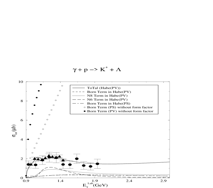
FIG. 3.: The total cross sections for dominant contributions (N6 and N8)and for PV- and PS-Born terms with and without form factors.

.

FIG. 4.: The differential cross sections for fixed kaon angles: $\theta=$ (a) $27^{\circ}$, (b) $90^{\circ}$, (c) $135^{\circ}$, and (d) $154^{\circ}$. Here we present the Habe(PV) with solid curve, the Ohta(PV) with dashed one. The long dashed and dot-dashed curves show the results of Noform(PV) and Noform(PS), respectively. The results of model 1 (AS1) in Ref. [14] are given by the dotted curves.

FIG. 5.: The differential cross sections at the fixed photon energy: $E_{\gamma}=$ (a) $1.01$, (b) $1.15$, (c) $1.243$, (d) $1.45$, (e) $1.8$, and (f) $2.1$ GeV. The lines are same as in Fig. 4.

.

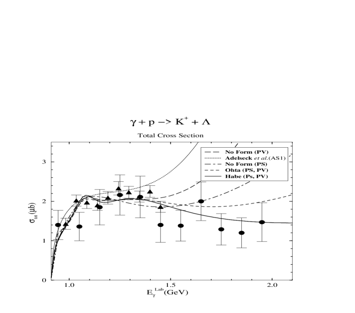
FIG. 6.: The total cross sections up to energy $E_{\gamma}$=2.1 GeV; lines as in Fig. 4.

.

FIG. 7.: The single polarization asymmetries: $\Lambda$-polarization asymmetry (P), target-polarization asymmetry (T), and beam-polarization asymmetry ($\Sigma$); (a),(b), and (c) are for angle fixed at $\theta$= $90^{o}$, and $E_{\gamma}$= (d) 1.2135 GeV, (e) 1.450 GeV, and (f) 1.450 GeV for the photon energy fixed; lines as in Fig. 4.

REFERENCES

• [1] Shigeo Hatsukade and Howard J. Schnitzer, Phys. Rev. 128, 468 (1962); Shigeo Hatsukade and Howard J. Schnitzer, Phys. Rev. 132, 1301 (1963).
• [2] N. F. Nelipa and V. A. Tsarev, Nucl. Phys. 45, 665(1963); N. F. Nelipa and V. A. Tsarev, Nucl. Phys. 55, 155 (1964); N. F. Nelipa, Nucl. Phys. 82, 680 (1966).
• [3] W. Schorsch, J. Tietge and W. Weilnböck, Nucl. Phys. B25, 179 (1970).
• [4] A. Kumar, Ph. D. Thesis, Ohio University (1994).
• [5] J. -F. Zhang, N. C. Mukhopadhyay and M. Benmerrouche, Phys. Rev. C 52, 1134 (1995).
• [6] D. Lu, R.H. Landau, and S.C. Phatak,Phys. Rev. C 52, 1662 (1995).
• [7] M. Gourdin and J. Dufour, Nuovo Cimento 26, 1410 (1963).
• [8] H. Thom, Phys. Rev. 151, 1322 (1966).
• [9] F. M. Renard and Y. Renard, Nucl. Phys. B25, 490 (1971); Y.Renard, ibid., B40, 499(1972).
• [10] R.A.Adelseck, C.Bennhold and L.E.Wright, Phys. Rev. C 32,1681(1985).
• [11] C. Bennhold and L. E. Wright, Phys. Rev. C36, 438 (1987).
• [12] C. Bennhold, Phys. Rev. C 39, 1994 (1989).
• [13] R. A. Adelseck and L.E.Wright, Phys. Rev. C 38, 1965(1988).
• [14] R. A. Adelseck and B. Saghai, Phys. Rev. C 42, 108 (1990).
• [15] R. A. Adelseck and B.Saghai, Phys. Rev. C45,2030(1992).
• [16] R.A.Williams, C.-R. Ji and S. R. Cotanch, Phys. Rev. C46, 1617 (1992) and S. R. Cotanch, R. A. Williams and C.-R. Ji, Phys. Scripta 48, 217(1993).
• [17] M. Bockhorst et al., Z. Phys. C 63, 37 (1994).
• [18] T. Mart, C. Bennhold and C.E. Hyde-Wright, Phys. Rev. C51, 1074 (1995).
• [19] B.Saghai and F.Tabakin, Phys. Rev. C 53, 66(1996).
• [20] J.-C.David, C.Fayard, G.H.Lamot and B.Saghai, Phys. Rev. C 53, 2613 (1996).
• [21] M. K. Cheoun, B. S. Han, B. G. Yu, and Il-Tong Cheon, Phys. Rev. C 54, 1811 (1996).
• [22] Bijan Saghai and Frank Tabakin, Phys. Rev. C 55, 917 (1997).
• [23] S.S. Hsiao and S.R. Cotanch, Phys. Rev. C 28, 1668 (1983).
• [24] S. Weinberg, Phys. Rev. Lett. 18 (1967) 188.
• [25] J.Cohen, Int. Journal of Modern Phys. 4, 1(1989) and Phys. Rev., C37, 187(1988).
• [26] J.L.Friar and B.F.Gibson, Phys. Rev. C15, 1779(1977).
• [27] P.de Baenst, Nucl. Phys. B24, 633(1970).
• [28] E. Mazzucato et al., Phys. Rev. Lett. 57, 3144 (1986);
• [29] Beck et al., Phys. Rev. Lett. 56, 1841 (1990).
• [30] J.C. Bergstrom et al., Phys. Rev. C53, R1052(1996).
• [31] H.W.Naus, J.H.Koch and J.L.Friar, Phys. Rev. C 41, 2852(1990).
• [32] S.Scherer and J.H.Koch, Nucl. Phys. A534, 461(1991).
• [33] D. Drechsel and L. Tiator, J. Phys. G18, 449 (1992).
• [34] S. Scherer, J. H. Koch, and J. L. Friar, Nucl. Phys. A 552, 515 (1993).
• [35] K. I. Blomqvist and J. M. Laget, Nucl. Phys. A280, 405 (1977).
• [36] T. Feuster and U. Mosel, Los Alamos eprint nucl-th/9803057.
• [37] K. Johnson and E.C.G Sudarshan, Ann. Phys. 13, 126 (1961).
• [38] G. Velo and D. Zwanziger, Phys. Rev. 186, 1337 (1969).
• [39] H. Burkhardt, J. Lowe, and A. A. Rosenthal, Nucl. Phys. A440, 653 (1985).
• [40] Bong Soo Han, Ph.D Thesis, Yonsei University, unpublished, (1999).
• [41] R.L. Workman and H.W. Fearing, Phys. Rev. D37, 3117(1988).
• [42] Fred de Jong and Rudi Malfliet, Phys. Rev. C 46 2567 (1992).
• [43] H. Tanabe, M. Kohno, and C. Bennhold, Phys. Rev C 39, 741 (1989).
• [44] C. Bennhold, T. Mart, and D. Kusno, Los Alamos eprint nuc-th/9703004 (1997).
• [45] H. Haberzettl, C. Bennhold, T. Mart, and T. Feuster, Few-Body Systems Suppl. 99, 1 (1998).
• [46] Nathan Isgur and Gabriel Karl, Phy. Lett. 72B, 109 (1977); Phys. Rev. D 18, 4187 (1978); Phys. Rev. D 19, 2653 (1979); Phys. Rev. D 20, 1191 (1979); Phys. Rev. D 21, 1868 (1980).
• [47] Jurij W. Darewych, Marko Horbatsch, and Roman Koniuk, Phys. Rev. D 28, 1125 (1983).
• [48] C. F. Chew, M. L. Goldberger, R. E. Low, and Y. Nambu, Phys. Rev. 106, 1345 (1957).
• [49] J. S. Ball, Phys. Rev. 124, 2014 (1961).
• [50] B.Krusche et al., Phys. Rev. Lett. 74, 3736(1995) and, ibid., 75, 3023(1995).
• [51] Jurij W. Darewych, Roman Koniuk, and Nathan Isgur, Phys. Rev. D32, 1765 (1985).
• [52] Particle Data Group, Phys. Rev. D50, 1994.
• [53] J. J. de Swart, Rev. Mod. Phys., 35, 916(1963).
• [54] Hartmut Pilkuhn, ”The Interactions of Hadrons”, North-Holland Publishing Company-Amstredam, 1967.
• [55] C. R. Ji and S. R. Cotanch, Phys. Rev. C 38, 2691 (1988).
• [56] R. D. Peccei, Phys. Rev. 176, 1812 (1968)
• [57] K. Ohta, Phys. Rev. C 40, 1335 (1989).
• [58] H. Haberzettl, Phys. Rev. C 56, 2041 (1997).
• [59] E. Kazes, Nuovo Cimento, 13, 899 (1959).
• [60] J. C. Ward, Phys. Rev. 78, 182 (1950); Y. Takahashi, Nuovo Cimento 6, 371 (1957).
• [61] R. L. Workman, H. W. L. Naus, S. J. Pollock, Phys. Rev. C 45, 2511 (1992).
• [62] S. Wang and M. K. Banergee, Phys. Rev. C 54, 2883 (1996).
• [63] D. D$\acute{e}$camp, B. Dudelzak, P. Eschstruth, and Th. Fourneron, Orsay Linear Accelerator Report LAL-1236, 1970; Th. Fourneron, Th$\acute{e}$se de Doctrat, d’Etat, Orsay Linear Accelerator Report LAL-1258, 1971.
• [64] F. James and M. Roos, MINUIT, CERN Report D506, 1981.
• [65] Particle Data Group, Euro. Phys. Jour. C3, (1998).
• [66] Xiadong Li, L.E.Wright and C.Bennhold, Phys. Rev. C 45, 2011(1992).
• [67] P.B.Siegel and B.Saghai, Phys. Rev. C52, 392(1995).
• [68] D.A.Whitehouse et al., Phys. Rev. Lett. 63, 1352(1989).
• [69] G. Niculescu et al., Phyc. Rev. Lett. 81, 1805 (1998).