Many-body corrections to the nuclear anapole moment II

Abstract

The contribution of many-body effects to the nuclear anapole moment were studied earlier in [1]. Here, more accurate calculation of the many-body contributions is presented, which goes beyond the constant density approximation for them used in [1]. The effects of pairing are now included. The accuracy of the short range limit of the parity violating nuclear forces is discussed.

BudkerINP 99 - 100

1 Introduction

In the previous paper [1], referred here as I, the contribution of the core nucleons to the anapole moment (AM), arising from the core polarization effects, has been calculated in the random-phase approximation (RPA). Recently, the first measurement of the AM of Cesium has been reported [2]. The immediate application of this measurement was the attempt to deduce the pion-nucleon weak parity-non-conserving (PNC) coupling constant $f_{\pi}$ [3], [4]. The comparison of the measured anapole moment value with the one calculated using a pure single-particle model leads to a value for $f_{\pi}$ that exceeds by a factor 4 the value deduced from a parity violating measurement in ${}^{18}F$ [5]. More sophisticated comparison was made in Ref. [6], where the results from ${}^{18}F$, the AM of ${}^{133}Cs$, and the upper bound for the AM of ${}^{205}Tl$ [7] were used to deduce both $f_{\pi}$ and $f_{\rho}$ PNC coupling constants. The combination of the coupling constants was found which satisfies both ${}^{18}F$ and ${}^{133}Cs$ experiments and which is barely in agreement with theory. These values, however, are inconsistent with the constraint obtained from ${}^{205}Tl$ measurement. This situation, even independently on ${}^{18}F$ experiments, raises the question how accurate is the theory of nuclear anapole moments. Here we address this question and present more accurate calculation of the many-body effects.

There are different contributions to the value of nuclear AM. The most significant and the least model dependent contribution comes from the valence nucleon. It is stable under variations of the single-particle potential [8]. Within the single-particle model it is often convenient to use the leading approximation (LA) [9] producing the simple analytical expression for the correction to the single-particle wave function $\delta\psi$ due to the PNC potential. The LA was used in I in calculations of the core nucleons contribution to the anapole moment. This is another contribution which is not negligible. The accuracy of the LA was estimated to be within 20% in [8]. We found, that although this is true for the upper level of the spin-orbit doublet, for the lower level the difference between LA and the exact correction $\delta\psi$ can be significant. This demands improving the calculation of the core nucleons contribution.

Another phenomenon that has to be accounted for is the pairing. The reason for this is that for ${}^{133}Cs$ nucleus there are single-particle states very close to the Fermi surface. The transitions to these states produce large contribution to the core polarization. In the presence of pairing these transitions will be strongly reduced, thus affecting the value of the polarization effects and the nuclear anapole moment.

Finally, we discuss the constants of the short range effective PNC interaction used in nuclear structure calculations. These constants were obtained from the finite range meson exchange forces by comparing typical matrix elements both finite range and short range interactions [10, 11, 12]. The factors $W_{\rho}\approx 0.4$ and $W_{\pi}\approx 0.16$ were found for $\pi$- and $\rho$-exchange forces. These values, however, were obtained for $\alpha$-particle and the extension to heavier nuclei should be checked separately. We found using the same procedure that the factor $W_{\pi}$ is state dependent and it is different for ${}^{133}Cs$ and ${}^{205}Tl$.

The paper is organized as follows. First, we discuss the accuracy of the LA. Then, we present the exact calculations of the core polarization contribution and demonstrate the necessity to include the pairing. Finally, we discuss the constants of the short range PNC interaction.

2 Core polarization contribution

For completeness of the discussion let us to remind the basic equations from I. There are several contributions to the AM arising from different parts of the electromagnetic current. Apart from magnetization current which gives the main contribution, there are contributions from the convection current, the spin-orbit current and the contact current arising from the momentum dependence of the corresponding parts of the Hamiltonian [8]:

$${\bf a}_{s}^{a} = \frac{\pi e\mu_{a}}{m}\mbox{\boldmath$r\times\sigma$}$$

$${\bf a}_{conv}^{p} = -\frac{\pi e}{m}\left\{{\bf p},(r^{2}-\frac{Z}{A}<r^{2}_{p}>)\right\}$$

$${\bf a}_{conv}^{n} = \frac{2\pi e}{m}\frac{Z}{A}<r^{2}_{p}>{\bf p}$$

$${\bf a}_{ls}^{p} = -\pi eU_{ls}^{pn}\rho_{0}\frac{N}{A}r^{2}\frac{df(r)}{dr}\mbox{\boldmath$\sigma\times n$}$$

$${\bf a}_{ls}^{n} = \pi eU_{ls}^{np}\rho_{0}\frac{Z}{A}\frac{d(r^{2}f(r))}{dr}\mbox{\boldmath$\sigma\times n$}$$

$${\bf a}^{p}_{c} = \frac{G_{F}}{\sqrt{2}}\frac{\pi e}{m}\rho_{0}g_{pn}\frac{N}{A}r^{2}f(r)\mbox{\boldmath$\sigma$}$$

$${\bf a}^{n}_{c} = \frac{G_{F}}{\sqrt{2}}\frac{\pi e}{m}\rho_{0}g_{np}\frac{Z}{A}r^{2}f(r)\mbox{ \boldmath$\sigma$}$$ (1)

Here $\{\;,\;\}$ is anticommutator, $<r^{2}_{p}>$ is the proton mean squared radius, $\rho_{0}$ is the central nuclear density, $f(r)=\rho(r)/\rho_{0}$ - nuclear density profile, and $U_{ls}^{pn}=U_{ls}^{np}=134\,MeV\cdot fm^{5}$ is the proton-neutron constant of the effective spin-orbit residual interaction [8]. $G_{F}$ is the weak interaction Fermi coupling constant, $m$ is the proton mass, and $\mu_{a}$ is the nucleon magnetic moment. The contact current contribution arises from the velocity dependence of the effective nucleon-nucleon PNC forces [8, 14]

The operators in Eq. (2) have 3 types of angular dependence. All of them, except the convection ones, are spin dependent. All of them except ${\bf a}_{c}$ are of E1 type. The operators created by the contact current are of M1 type. The convection terms in Eq. (2) differ from the one used in I and [8]. Here we accounted for the recoil correction by subtracting the part related to the motion of a nucleus as a whole.

As in I, we use for the radial dependence of the effective operators related to Eq. (2) the notation $V[{\bf a}_{i}]({\bf r})$. The RPA equations for the effective radial fields $V[{\bf a}_{i}]({\bf r})$ are (see Eqs. (17),(18) in I)

$$V=V_{0}([{\bf a}_{i}])+F_{s}\,A\,V,$$ (2)

$$\delta V=F_{w}\,AV+F_{s}\,\delta AV+F_{s}\,A\delta V.$$ (3)

Here $F_{w}$ is the PNC nucleon-nucleon interaction

$$F_{w}=\frac{G}{\sqrt{2}}\frac{1}{4m}\sum_{a,b}\left(\{(g_{ab}\mbox{\boldmath$\sigma$}_{a}-g_{ba}\mbox{\boldmath$\sigma$}_{b})\cdot({\bf p}_{a}-{\bf p}_{b}),\delta({\bf r}_{a}-{\bf r}_{b})\}\right.$$

$$\left.+\ g^{\prime}_{ab}\mbox{\boldmath$[\sigma_{a}\times\sigma_{b}]$}\cdot\mbox{\boldmath$\nabla$}\delta({\bf r}_{a}-{\bf r}_{b})\right),$$ (4)

and $F_{s}$ is the residual spin-spin interaction

$$F_{s}(ab)=C\,\left(g_{0}+g^{\prime}_{0}\mbox{\boldmath$\tau_{a}\cdot\tau_{b}$}\right)\mbox{\boldmath$\sigma_{a}\cdot\sigma_{b}$}\delta({\bf r}_{a}-{\bf r}_{b}).$$ (5)

As in I, we use $C=300\;MeV\cdot fm^{3}$, $g_{0}=0.6$, and $g_{0}^{\prime}=1$. Averaging the interaction Eq.(4) over core particles we obtain a single-particle PNC potential

$$W_{a}({\bf r})=\frac{G}{\sqrt{2}}\frac{g_{a}\rho_{0}}{2m}\{(\mbox{\boldmath$\sigma$}\cdot{\bf p}),f(r)\},$$ (6)

where $\rho_{0}$ is the central nuclear density, $f(r)$ is the nuclear density profile and the constants $g_{a}$ are related to the interaction constants $g_{ab}$ (see Eq. (4) in I). In the absence of pairing, the static particle-hole propagator $A({\bf r},{\bf r}^{\prime})$ has the form

$$A({\bf r},{\bf r}^{\prime})=\sum_{\nu\nu^{\prime}}\psi_{\nu}({\bf r})\psi^{\dagger}_{\nu}({\bf r}^{\prime})\frac{n_{\nu}-n_{\nu^{\prime}}}{\epsilon_{\nu}-\epsilon_{\nu^{\prime}}}\psi_{\nu^{\prime}}({\bf r}^{\prime})\psi^{\dagger}_{\nu^{\prime}}({\bf r}),$$ (7)

where $n_{\nu}$ are the occupation numbers, $\epsilon_{\nu}$ and $\psi_{\nu}({\bf r})$ are the energies and the wave functions of the single-particle levels. The Feynman diagrams corresponding to Eq.(2,3) are shown in Fig.1.

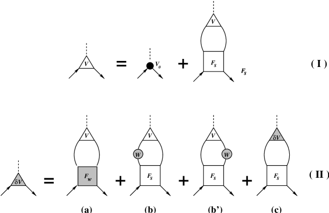
Figure 1: Feynman diagrams corresponding to Eqs.(2),(3).
I. The anapole moment renormalization diagram describing the core polarization effects. The filled circle is the bare anapole operator. The open triangle is the dressed one. The open square is the spin-spin residual strong interaction.
II. Additional contribution to the anapole moment due to parity violation in the core states. a) - the direct contribution of the two-particle effective PNC interaction. b) and b’) - the effective contribution due to parity violation in the core states. c) - the renormalization diagram. The shaded circle is the single-particle PNC interaction. The shaded square is the two-particle effective PNC interaction.

Eq.(2), which is shown in the top diagrams (I) in Fig.1, describes the usual RPA renormalization of the bare operator $V_{0}[{\bf a}_{i}]({\bf r})$. The next Eq.(3), which is shown in the bottom diagrams (II) in Fig.1, describes an additional contribution from the core nucleons arising both from the direct P-odd nucleon-nucleon interaction $F_{w}$, see Fig.1 (II a), and from the P-even residual interaction via admixture of opposite parity states to the wave functions of the core nucleons,see Fig.1 (II b), (II b’). The last term in Eq.(3), see Fig.1 (II c), is responsible for the renormalization of these contributions.

It is worth mentioning that the correction $\delta V$ has the parity opposite to $V$. The change in parity happens because $\delta V$ is created from $V$ by the interaction that does not conserve parity. While AM is E1 type operator, the correction $\delta V$ is M1 type. For this reason the renormalization due to the core polarization will be different for $V$ and $\delta V$, since different transitions are involved in the kernels of integral equations (2) and (3). Eq.(2) describes also the renormalization of the operators ${\bf a}_{c}$. They don’t have $\delta V$ since they themselves are of first order in the weak PNC interaction. The AM value is given by the sum of all these terms:

$$a_{i}=\langle\delta\psi|V[{\bf a}_{i}]|\psi\rangle+\langle\psi|V[{\bf a}_{i}]|\delta\psi\rangle+\langle\psi|\delta V[{\bf a}_{i}]|\psi\rangle,$$ (8)

where the index i means here $s$, $conv$ or $ls$. For the contact contribution we have

$$a_{c}=\langle\psi|V[{\bf a}_{c}]|\psi\rangle.$$

2.1 Leading approximation accuracy

Eq.(3) was solved in I using LA in calculations of $\delta A$. The accuracy of LA was estimated in [8] within 20%. This estimate was maid for odd valence nucleons in a set of nuclei. Occasionally, all the valence nucleon levels under discussion were the upper levels of the spin-orbit doublet. The typical difference between exact $\delta R(r)$ and $rR(r)$ in LA for the upper level of the spin-orbit doublet is shown in the left plot of Fig.2.

Figure 2: Admixture of the opposite parity $\delta R(r)$ for different components of the spin-orbit doublets. Left panel - 2d_3/2 level, right panel - 1g_9/2 level. LA is shown by the dashed lines. Full lines show the exact solution.

However, the sum in $\delta A$ goes over all states. For the lower states of the doublet the difference in the peak heights can reach a factor 2 as one can see in the right plot in Fig.2. In all cases the exact correction and the LA are peaked near the surface. However, the ratio of the peak heights differs considerably for the upper and the lower states of spin-orbit doublets.

The systematic study of this ratio is presented in Fig. 3.

Figure 3: Ratio $\zeta$ of the maximum in exact $\delta R(r)$ to the maximum in $\delta R(r)$ found in LA for a set of the proton single-particle orbitals.

Here we plotted the ratio of the peak heights of the exact $\delta R(r)$ and $rR(r)$ in the LA for a set of proton states in the Woods-Saxon potential. While for the states with $j=l-1/2$ the ratio remains close to 1, for the states with $j=l+1/2$ the ratio goes down with increasing orbital angular momentum $l$. For the state $1h_{11/2}$ the exact correction $\delta R(r)$ differs more than by factor 2 from the correction $rR(r)$ calculated using LA. From these results we see that the estimated accuracy 20% in calculation of $\delta A$ cited in I is too optimistic and more accurate calculation is necessary.

2.2 Exact $\delta A$

Let us start with the expression $F_{s}AV$ in Eq.(2). In coordinate space it can be presented as follows

$$(F_{s}AV[{\bf a}_{i}])_{b}({\bf r})=Cg^{bc}_{0}\mbox{\boldmath$\sigma$}{\bf X}_{c}({\bf r}),$$

where $C$ and $g_{bc}$ are the parameters of the residual interaction (5), and

$${\bf X}({\bf r})=\sum_{\nu\nu^{\prime}}\frac{n_{\nu}-n_{\nu^{\prime}}}{\epsilon_{\nu}-\epsilon_{\nu^{\prime}}+\omega}\int\;d^{3}r^{\prime}\;\psi^{\dagger}_{\nu}({\bf r})\mbox{\boldmath$\sigma$}\psi_{\nu^{\prime}}({\bf r})\psi^{\dagger}_{\nu^{\prime}}({\bf r}^{\prime})V({\bf r}^{\prime})\psi_{\nu}({\bf r}^{\prime}).$$ (9)

In the following derivation we keep the external frequency $\omega$. It will be put to zero in the final result. Introducing the single-particle Green’s function

$$G({\bf r\;r}^{\prime}|E)=\sum_{\nu}\frac{\psi_{\nu}({\bf r})\psi^{\dagger}_{\nu}({\bf r}^{\prime})}{E-\epsilon_{\nu}}$$

we can rewrite the Eq.(9) in the following form

$${\bf X}({\bf r})=\sum_{\nu}n_{\nu}\,\int\;d^{3}r\;\left\{\psi^{\dagger}_{\nu}({\bf r})\mbox{\boldmath$\sigma$}G({\bf r\;r}^{\prime}|\epsilon_{\nu}+\omega)V({\bf r}^{\prime})\psi_{\nu}({\bf r}^{\prime})\right.$$

$$+\left.\psi^{\dagger}_{\nu}({\bf r}^{\prime})V({\bf r}^{\prime})G({\bf r}^{\prime}\;{\bf r}|\epsilon_{\nu}-\omega)\mbox{\boldmath$\sigma$}\psi_{\nu}({\bf r})\right\}.$$ (10)

The correction to Eq.(10) arising from the single-particle PNC potential can be obtained using the correction to the single-particle wave function $\psi_{\nu}({\bf r})$ defined in I:

$$\delta\psi_{\nu}({\bf r})=-\imath\xi_{a}(\mbox{\boldmath$\sigma$}{\bf n})\delta R_{\nu}(r)\Omega_{\nu}({\bf n})=\imath\xi_{a}\delta R_{\nu}(r)\Omega_{\tilde{\nu}}({\bf n}),$$ (11)

where

$$\xi_{a}=\frac{G}{\sqrt{2}}g_{a}\rho_{0}.$$

We used here the relation

$$\Omega_{j\tilde{l}m}({\bf n})=-(\mbox{\boldmath$\sigma$}{\bf n})\Omega_{jlm}({\bf n}),$$

where $\tilde{l}=2j-l$. For the correction $\delta{\bf X}({\bf r})$ we find then

$$\delta{\bf X}({\bf r})=\delta{\bf X}_{1}({\bf r})+\delta{\bf X}_{2}({\bf r}),$$

where

$$\delta{\bf X}_{1}({\bf r})=\imath\xi\sum_{\nu\nu^{\prime}}n_{\nu}\int r^{\prime 2}dr^{\prime}$$

$$\times\left\{(\Omega^{\dagger}_{\nu}({\bf n})\mbox{\boldmath$\sigma$}\Omega_{\nu^{\prime}}({\bf n}))G_{\nu^{\prime}}(r,r^{\prime}|\epsilon_{\nu}+\omega)<\nu^{\prime}|V({\bf r}^{\prime})|\tilde{\nu}>\delta R_{\nu}(r^{\prime})R_{\nu}(r)\right.$$

$$-\ (\Omega^{\dagger}_{\tilde{\nu}}({\bf n})\mbox{\boldmath$\sigma$}\Omega_{\nu^{\prime}}({\bf n}))G_{\nu^{\prime}}(r,r^{\prime}|\epsilon_{\nu}+\omega)<\nu^{\prime}|V({\bf r}^{\prime})|\nu>\delta R_{\nu}(r)R_{\nu}(r^{\prime})$$

$$+\ \delta R_{\nu}(r)R_{\nu}(r^{\prime})<\nu|V({\bf r}^{\prime})|\nu^{\prime}>(\Omega^{\dagger}_{\nu^{\prime}}({\bf n})\mbox{\boldmath$\sigma$}\Omega_{\tilde{\nu}}({\bf n}))G_{\nu^{\prime}}(r^{\prime}r|\epsilon_{\nu}-\omega)$$

$$\left.\ \ \ \ \ \ \ \ -\ R_{\nu}(r)\delta R_{\nu}(r^{\prime})<\tilde{\nu}|V({\bf r}^{\prime})|\nu^{\prime}>(\Omega^{\dagger}_{\nu^{\prime}}({\bf n})\mbox{\boldmath$\sigma$}\Omega_{\nu}({\bf n}))G_{\nu^{\prime}}(r^{\prime}r|\epsilon_{\nu}-\omega)\right\},$$ (12)

and

$$\delta{\bf X}_{2}({\bf r})=\sum_{\nu}n_{\nu}\int d^{3}r^{\prime}\left\{\psi^{\dagger}_{\nu}({\bf r})\mbox{\boldmath$\sigma$}\delta G({\bf r\,r}^{\prime}|\epsilon_{\nu}+\omega)V({\bf r}^{\prime})\psi_{\nu}({\bf r}^{\prime})\right.$$

$$\left.+\ \psi^{\dagger}_{\nu}({\bf r}^{\prime})V({\bf r}^{\prime})\delta G({\bf r\,r}^{\prime}|\epsilon_{\nu}-\omega)\mbox{\boldmath$\sigma$}\psi_{\nu}({\bf r})\right\}.$$ (13)

The angular brackets in Eq.(12) denote the matrix elements in angular and spin variables only. In the following calculations for spherical nuclei, it is convenient to separate the angular variables by expanding both $\delta{\bf X}_{1}({\bf r})$ and $\delta{\bf X}_{2}({\bf r})$ in a set of the vector spherical harmonics ${\bf Y}^{L}_{JM}({\bf n})$,

$$\delta{\bf X}_{i}({\bf r})=\sum_{L}X_{i}^{L}(r){\bf Y}^{L}_{JM}({\bf n}).$$ (14)

In Eq.(14) the total angular momentum $J$ is fixed, $J=1$, and the sum goes over $L$ only. Multiplying Eqs. (12 -13) by ${\bf Y}^{L\dagger}_{JM}({\bf n})$, integrating over angles and separating the dependence on all angular momentum projections $M$ via Wigner-Eckart theorem, we obtain for the reduced functions of $r$

$$X^{L}_{1}(r)=\frac{\imath\xi}{3}\sum_{\nu\nu^{\prime}}n_{\nu}\int r^{\prime 2}\,dr^{\prime}\left\{\delta R_{\nu}(r)R_{\nu}(r^{\prime})(\nu||V(r^{\prime})||\nu^{\prime})(\tilde{\nu}||T^{L}_{1}||\nu^{\prime})\right.$$

$$\left.-\ \delta R_{\nu}(r^{\prime})R_{\nu}(r)(\tilde{\nu}||V(r^{\prime})||\nu^{\prime})(\nu||T^{L}_{1}||\nu^{\prime})\right\}$$

$$\times\ \bigl{(}G_{\nu^{\prime}}(r,r^{\prime}|\epsilon_{\nu}+\omega)+G_{\nu^{\prime}}(r,r^{\prime}|\epsilon_{\nu}-\omega)\bigr{)}.$$ (15)

Here, double vertical lines mean the reduced angular matrix elements. The tensor operators $T^{L}_{JM}$ are defined as in I:

$$T^{L}_{JM}=\{\sigma\otimes Y_{L}\}_{JM}$$ (16)

Similar expression can be obtained for $X^{L}_{2}(r)$:

$$X^{L}_{2}(r)=\frac{1}{3}\sum_{\nu\nu^{\prime}}n_{\nu}(\nu^{\prime}||T^{L}_{1}||\nu)R_{\nu}(r)$$

$$\times\int r^{\prime 2}dr^{\prime}\bigl{(}\delta G_{\nu^{\prime}\tilde{\nu^{\prime}}}(r,r^{\prime}|\epsilon_{\nu}+\omega)+\delta G_{\nu^{\prime}\tilde{\nu^{\prime}}}(r,r^{\prime}|\epsilon_{\nu}-\omega)\bigr{)}(\tilde{\nu^{\prime}}||V(r^{\prime})||\nu)R_{\nu}(r^{\prime}).$$ (17)

In Eqs.(13,17) $\delta G$ is the correction to the Green’s function of the Schrödinger equation for single-particle orbitals due to the PNC potential Eq.(6). In first order the correction is

$$\delta G({\bf r},{\bf r}^{\prime})=\int\,d^{3}xG({\bf r},{\bf x})W({\bf x})G({\bf x},{\bf r}^{\prime})$$

Separating the angular dependence we obtain for the radial correction

$$\delta G_{\nu\tilde{\nu}}(r,r^{\prime})=\frac{\imath\xi}{2m}\int_{0}^{\infty}x^{2}dx\,f(x)\left(G_{\nu}(r,x)(\frac{\begin{array}[]{c}{\leftarrow\rightarrow}\\ \partial\end{array}}{\partial x}-\frac{2k}{x})G_{\tilde{\nu}}(x,r^{\prime})\right).$$ (18)

Here $k=(l-j)(2j+1)$. For obvious reason the, PNC potential couples only the states with the angular momenta $l$ and $\tilde{l}$.

The final equations for the radial functions $v[{\bf a}_{i}](r)$ and $\delta v_{L}[{\bf a}_{i}](r)$ are as follows

$$v^{a}[{\bf a}_{i}](r)-\sum_{b=p,n}g_{0}^{ab}\int_{0}^{\infty}r^{\prime 2}dr^{\prime}\,A^{b}_{11}(r,r^{\prime})v^{b}[{\bf a}_{i}](r^{\prime})=v^{a}_{0}[{\bf a}_{i}](r);$$ (19)

$$\delta v_{L}^{a}[{\bf a}_{i}](r)-\sum_{b=p,n}g_{0}^{ab}\sum_{L^{\prime}=0,2}\int_{0}^{\infty}r^{\prime 2}dr^{\prime}\,A_{LL^{\prime}}^{b}(r,r^{\prime})\delta v_{L^{\prime}}^{a}[{\bf a}_{i}](r^{\prime})=\delta v_{L}^{0a}[{\bf a}_{i}](r),$$ (20)

where the radial particle-hole propagator $A_{LL^{\prime}}^{b}(r,r^{\prime})$ is

$$A_{LL^{\prime}}^{b}(r,r^{\prime})=\frac{1}{3}C\sum_{jlnj^{\prime}l^{\prime}}n^{b}_{jln}\langle jl||T^{L}_{1}||j^{\prime}l^{\prime}\rangle\langle jl||T^{L^{\prime}}_{1}||j^{\prime}l^{\prime}\rangle^{*}R_{jln}(r)R_{jln}(r^{\prime})$$

$$\times\ \bigl{(}G_{j^{\prime}l^{\prime}}(r,r^{\prime};\epsilon_{jln}+\omega)+G_{j^{\prime}l^{\prime}}(r,r^{\prime};\epsilon_{jln}-\omega)\bigr{)},$$ (21)

with $\omega\rightarrow 0$. Here $C$ is the normalization constant of the residual interaction Eq.(5) and $G_{jl}(r,r^{\prime};\epsilon)$ is Green’s function of the radial Schrödinger equation.

Eqs.(19),(20) are similar for all anapole operators Eq.(2), except for the convection current operator which will be treated separately. The right-hand-side of Eq.(19) for the spin current anapole operator is

$$v^{a}_{0}[{\bf a}_{s}](r)=-\imath\sqrt{\frac{8\pi}{3}}\frac{\pi e\mu_{a}}{m}r.$$ (22)

The transition from the Cartesian vector product in Eq.(2) to the tensor operator $T^{1}_{1M}$ results in the factor $-\imath\sqrt{8\pi/3}$. The factor is common for the spin and spin-orbit anapole operators. The radial dependence follows Eq.(2). The right-hand-side of Eq.(20) is given by

$$\delta v^{0a}_{L}[{\bf a}_{i}](r)=C\sum_{b=p,n}g_{0}^{ab}(X_{1,b}^{L}(r)+X_{2,b}^{L}(r)).$$ (23)

In Eq.(23) we omit the direct contribution of the two-particle effective PNC interaction corresponding to the diagram (IIa) in Fig.1. According to the estimates made in Ref.[13] this contribution is small, it does not have the factor $A^{2/3}$. The estimate in [13] was obtained with harmonic oscillator wave functions. We calculated the diagram (IIa) for $V^{0}[{\bf a}_{s}]$ from Eq.(2) with the Woods-Saxon wave functions. For ¹³³Cs nucleus we obtained the contribution

$$\delta\kappa_{F_{w}}=(-4.1g_{pp}+0.1g_{pn}+4.9g_{np}-1.6g^{\prime}_{pn})\cdot 10^{-3}=-0.015$$

for the ”best values” of the coupling constants [18]. This number should be compared with the single-particle value of $\kappa_{s}=0.32$, and it gives the contribution less than $5\%$. Similar calculations give $\delta\kappa_{F_{w}}=0.003$ for ${}^{205}Tl$, $\delta\kappa_{F_{w}}=0.023$ for ${}^{209}Bi$, and $\delta\kappa_{F_{w}}=0.0085$ for ${}^{207}Pb$. All these values are in agreement with the estimates of Ref.[13].

The convection current anapole operator Eq.(2) expressed via tensor operators has the form

$$(a^{p}_{conv})_{M}=-\imath\sqrt{\frac{8\pi}{3}}\frac{\pi e}{m}\left(\frac{r^{2}-\frac{Z}{A}<r_{p}^{2}>}{2r}\{\right.{\bf l},{\bf Y}^{1}_{1M}\}$$

$$-\ \frac{1}{\sqrt{8}}\{\frac{\partial}{\partial r}\left.+\frac{1}{r},r^{2}-\frac{Z}{A}<r_{p}^{2}>\}Y_{1M}\right).$$ (24)

$$(a^{n}_{conv})_{M}=\imath\sqrt{\frac{8\pi}{3}}\frac{\pi e}{m}\frac{Z}{A}<r_{p}^{2}>\left(\frac{1}{2r}\{{\bf l},{\bf Y}^{1}_{1M}\}-\frac{1}{\sqrt{2}}(\frac{\partial}{\partial r}+\frac{1}{r})Y_{1M}\right).$$

The operators Eq.(24) are non-local and do not include spin. For the last reason they are not renormalized directly by the residual interaction Eq.(5). However, due to the spin-orbit potential a new spin dependent contribution to AM is generated in first order in the residual interaction Eq.(5). Its tensor structure is given by the same tensor operator as that for the spin current AM ${\bf a}_{s}$. The radial dependence of this polarization contribution is given by

$$v^{a0}_{pol}(r)=\frac{C}{3}\sum_{b=p,n}g_{0}^{ab}\sum_{\nu\nu^{\prime}}n_{\nu}R_{\nu}(r)(\nu||T^{1}_{1}||\nu^{\prime})^{*}$$

$$\times\int_{0}^{\infty}r^{\prime 2}dr^{\prime}R_{\nu}(r^{\prime})(\nu||a^{b}_{conv}||\nu^{\prime})\bigl{(}G_{\nu^{\prime}}(r^{\prime},r|\epsilon_{\nu}+\omega)+G_{\nu^{\prime}}(r,r^{\prime}|\epsilon_{\nu}-\omega)\bigr{)},$$ (25)

where $\omega\rightarrow 0$. This operator undergoes the usual renormalization described by Eq.(19) producing in the next orders in the residual interaction the renormalized radial operator $v_{pol}^{a}(r)$. Although the direct contribution of the convection current to AM is small, the polarization contribution Eq.(25) is larger and has to be included. Total operator generated by the convection current has the following structure

$$v^{b}[{\bf a}_{conv}](r)=a^{b}_{conv}+v^{b}_{pol}(r)T_{1}^{1},$$ (26)

where $a^{b}_{conv}$ is given by Eq.(24) and $v^{b}_{pol}(r)$ is the dressed polarization operator Eq.(25). The tensor operator $T_{1}^{1}$ is defined by Eq.(16) and we omit the total momentum projection. This very operator Eq.(26) should be used in the Eq.(23) for the right-hand-side of Eq.(20).

The values of the AM resulting from the solutions of Eqs.(19), (20) are summarized in Table 1 and Table 2 for ${}^{133}Cs$ and ${}^{205}Tl$ nuclei. For comparison, in the row labeled by I we listed the results of previous calculation with the use of LA. The results of present calculations are listed in the row labeled by II.

The value cited in column $V-V_{0}$ is the renormalization of the single-particle (column s.p.) value due to the core polarization by Eq.(3). One can see that the polarization contribution is about half of the single-particle one and it has an opposite sign compared to the single-particle contribution for all spin dependent operators. This is in accordance with the repulsive nature of the spin-spin residual interaction Eq.(5). In this case the core produces a screening of the valence nucleon spin.

The contribution of the convection current in the Tables 1 and 2 was listed together with the polarization effects discussed above. The single-particle value is small compared to the magnetization current contribution. Let us note that it differs from the corresponding value cited in I. The difference, although small, comes from the center of-mass-motion that was not excluded in I. It is interesting to note that for the convection current, the polarization contribution has the same sign as the single-particle one. This is in contrast to the spin case where the polarization contribution has always the opposite sign compared to the single-particle value. The difference between these two cases lies in the polarization loop which is non-diagonal for the convection current case. It has the spin operator in one vertex and the convection part of the AM (see Eq.(2)) in the other. For such non-diagonal loop the sign is not fixed.

The main conclusion that can be drawn from the present results is that the LA overestimates the contribution of $\delta V$ approximately by a factor 2. The summed value $\kappa_{tot}$ has decreased by 50%, as compared to its single-particle value. Thus, the effect of the core polarization is considerable.

3 Pairing effects

In general, the pairing effects are important only for the transitions near the Fermi surface. Therefore, they can be neglected in calculations of $\delta\psi$ and in the polarization loop in Eq.(19) where the transitions to at least next shell are involved. The situation is different for Eq.(20) where the transitions within the open shell are allowed. Good example is ${}^{133}Cs$ where the polarization loop includes the transitions between the states with the excitation energy about one hundred KeV. Transitions to such close levels contribute significantly into polarization loop creating large response in $\delta V$. These transitions will apparently be suppressed by pairing correlations. For these reason the polarization loop in Eq.(20) should be modified in order to include pairing.

The modification is straightforward and can be done similarly to [15]. The particle-hole propagator for a T-odd channel in the presence of pairing has the form

$$A({\bf r},{\bf r^{\prime}})=-\sum_{\nu\nu^{\prime}}\frac{(u_{\nu}v_{\nu^{\prime}}-v_{\nu}u_{\nu^{\prime}})^{2}\psi_{\nu}({\bf r})\psi^{\dagger}_{\nu^{\prime}}({\bf r})\psi_{\nu^{\prime}}({\bf r^{\prime}})\psi^{\dagger}_{\nu}({\bf r^{\prime}})}{E_{\nu}+E_{\nu^{\prime}}},$$ (27)

where $u_{\nu}$ and $v_{\nu}$ are the Bogolyubov factors, and $E_{\nu}=\sqrt{(\epsilon_{\nu}-\mu)^{2}+\Delta^{2}}$ where $\Delta$ and $\mu$ are the pairing gap and the chemical potential. Below, we shall neglect slight state dependence of the pairing gap and put $\Delta=const$. Let us divide the single-particle space into 3 regions. Let $P_{\nu}$ be a projection operator onto the region near the Fermi surface, where pairing produces a significant effect. It is convenient to include here all bound states above the Fermi surface. Let $Q_{\nu}$ be a projection operator onto the hole states below the pairing region. In this region we neglect the pairing effects. The states in continuum will be projected by $1-P_{\nu}-Q_{\nu}$. Introducing the identity

$$1=(P_{\nu}+Q_{\nu}+1-P_{\nu}-Q_{\nu})(P_{\nu^{\prime}}+Q_{\nu^{\prime}}+1-P_{\nu^{\prime}}-Q_{\nu^{\prime}})$$

into Eq.(27) we obtain the expression for the particle-hole loop as a sum of 7 following terms

$$A({\bf r},{\bf r^{\prime}})=-\sum_{\nu\nu^{\prime}}\psi_{\nu}({\bf r})\psi^{\dagger}_{\nu^{\prime}}({\bf r})\psi_{\nu^{\prime}}({\bf r^{\prime}})\psi^{\dagger}_{\nu}({\bf r^{\prime}})\times\left\{\frac{(u_{\nu}v_{\nu^{\prime}}-v_{\nu}u_{\nu^{\prime}})^{2}}{E_{\nu}+E_{\nu^{\prime}}}P_{\nu}P_{\nu^{\prime}}\right.$$

$$+\frac{u_{\nu}^{2}}{E_{\nu}-\epsilon_{\nu^{\prime}}+\mu}P_{\nu}Q_{\nu^{\prime}}+\frac{u_{\nu^{\prime}}^{2}}{E_{\nu^{\prime}}-\epsilon_{\nu}+\mu}P_{\nu^{\prime}}Q_{\nu}$$

$$+\frac{v_{\nu}^{2}}{E_{\nu}+\epsilon_{\nu^{\prime}}-\mu}P_{\nu}(1-P_{\nu^{\prime}}-Q_{\nu^{\prime}})+\frac{v_{\nu^{\prime}}^{2}}{E_{\nu^{\prime}}+\epsilon_{\nu}-\mu}P_{\nu^{\prime}}(1-P_{\nu}-Q_{\nu})$$

$$\left.-\frac{1}{\epsilon_{\nu^{\prime}}-\epsilon_{\nu}}Q_{\nu^{\prime}}(1-P_{\nu}-Q_{\nu})-\frac{1}{\epsilon_{\nu}-\epsilon_{\nu^{\prime}}}Q_{\nu}(1-P_{\nu^{\prime}}-Q_{\nu^{\prime}})\right\}.$$ (28)

In Eq.(28) we put $\Delta=0$ in all terms containing $Q_{\nu}$. The sum over the whole single-particle space is present in the last 4 terms containing the unit projection operator. Combining these terms together we can present Eq.(28) as a sum of three different terms

$$A({\bf r},{\bf r}^{\prime})=A_{Q}({\bf r},{\bf r}^{\prime})+A_{P}({\bf r},{\bf r}^{\prime})+A_{\theta}({\bf r},{\bf r}^{\prime}),$$

where

$$A_{Q}({\bf r},{\bf r}^{\prime})=\sum_{\nu}Q_{\nu}\{\psi_{\nu}({\bf r})\psi_{\nu}^{\dagger}({\bf r}^{\prime})G({\bf r}^{\prime},{\bf r}|\epsilon_{\nu})+G({\bf r},{\bf r}^{\prime}|\epsilon_{\nu})\psi_{\nu}({\bf r}^{\prime})\psi_{\nu}^{\dagger}({\bf r})\}$$ (29)

includes the transitions from the deep holes,

$$A_{P}({\bf r},{\bf r}^{\prime})=-\sum_{\nu}P_{\nu}v_{\nu}^{2}\{\psi_{\nu}({\bf r})\psi_{\nu}^{\dagger}({\bf r}^{\prime})G({\bf r}^{\prime},{\bf r}|\mu-E_{\nu})+G({\bf r},{\bf r}^{\prime}|\mu-E_{\nu})\psi_{\nu}({\bf r}^{\prime})\psi_{\nu}^{\dagger}({\bf r})\}$$ (30)

includes the transitions from the pairing region, and

$$A_{\theta}({\bf r},{\bf r}^{\prime})=-\sum_{\nu\nu^{\prime}}\psi_{\nu}({\bf r})\psi_{\nu}^{\dagger}({\bf r}^{\prime})\Theta_{\nu\nu^{\prime}}\psi_{\nu}({\bf r}^{\prime})\psi_{\nu}^{\dagger}({\bf r})$$ (31)

with

$$\Theta_{\nu\nu^{\prime}}=[\frac{(u_{\nu}v_{\nu^{\prime}}-v_{\nu}u_{\nu^{\prime}})^{2}}{E_{\nu}+E_{\nu}^{\prime}}-\frac{v_{\nu}^{2}}{E_{\nu}-\epsilon_{\nu^{\prime}}+\mu}-\frac{v_{\nu^{\prime}}^{2}}{E_{\nu^{\prime}}-\epsilon_{\nu}+\mu}]P_{\nu}P_{\nu^{\prime}}$$

$$+[\frac{u_{\nu}^{2}}{E_{\nu}-\epsilon_{\nu^{\prime}}+\mu}-\frac{v_{\nu}^{2}}{E_{\nu}+\epsilon_{\nu^{\prime}}-\mu}+\frac{1}{\epsilon_{\nu^{\prime}}-\epsilon_{\nu}}]P_{\nu}Q_{\nu^{\prime}}$$

$$+[\frac{u_{\nu^{\prime}}^{2}}{E_{\nu^{\prime}}-\epsilon_{\nu}+\mu}-\frac{v_{\nu^{\prime}}^{2}}{E_{\nu^{\prime}}+\epsilon_{\nu}-\mu}+\frac{1}{\epsilon_{\nu}-\epsilon_{\nu^{\prime}}}]P_{\nu^{\prime}}Q_{\nu}.$$

includes the transitions from the pairing regions to the region of deep holes. In all these terms the sum goes over a finite range of the single-particle space and can be calculated directly.

Strictly speaking, in the presence of pairing the particle-particle channel should be added to Eq.(25) and the equation for $V$ has to be modified. With the particle-particle channel a new interaction $F^{\xi}$ appears and the total number of equations doubles. The parameters of the interaction $F^{\xi}$ can be found from masses of the nuclei that differ by two protons or two neutrons [16]. This procedure, however, determines the spin-independent part of the interaction $F^{\xi}$. The spin-independent interaction in the short-range approximation does not renormalize the spin-dependent operators. As for the spin-dependent part of $F^{\xi}$, its magnitude remains unknown up to now and for this reason we did not include it in our equations.

For the right-hand-side of Eq.(23) one can obtain $\delta A$ from Eqs.(29)-(31) using in first order $\delta\psi$ by Eq.(11) and $\delta G$ by Eq.(18).

In Fig.4 we plot the difference $v^{p}_{s}(r)-v^{p}_{0s}(r)$ for the spin part of the AM operator both in the absence and in the presence of pairing. As expected, the difference between these two cases is insignificant. For $\delta V$ the situation is somewhat different. In Fig.5 we plot the right-hand-side of Eq.(23) for the transitions with $L=0$ (left plot). In this case the difference is also small. However, for the transitions with $L=2$ (right plot) the difference is significant. This is the direct influence of pairing that reduces the transitions to closely lying levels. The final value of AM does not changed strongly because the contribution of $X^{L}[v^{p}_{0s}]$ with $L=2$ to AM is small.

Figure 4: The difference $v^{p}_{s}(r)-v^{p}_{0s}(r)$ for the spin part of the AM operator in the presence of pairing (solid line), and in the absence of pairing (dashed line).

Figure 5: The contributions to proton $X^{L}[v^{p}_{0s}]$ with different $L$ in the absence (dashed line), and the presence (solid line) of pairing. The interaction constant $g_{p}$ put equal to $1$ for illustrative purpose. On the left plot $L=0$, on the right plot $L=2$.

The results of the anapole moment calculations with pairing are listed in the Table 1 for ${}^{133}Cs$ nucleus in the row labeled III. For the pairing gap $\Delta$ we used the values $\Delta_{p}=0.95MeV$ for protons and $\Delta_{n}=1.05MeV$ for neutrons from Ref.[17]. As expected, the pairing does not influence much the matrix element of the anapole moment operator $V$. For $\delta V$ the effects are relatively larger. As mentioned above, the pairing reduces the transitions near the Fermi surface with small $\Delta E$. For the $Cs$ nucleus this happens only for the proton transition $1g_{7/2}-2d_{5/2}$, $\Delta l=2$ that does not contribute significantly to the anapole moment.

4 Parameters of the PNC nuclear forces

The constants $g_{ab}$ and $g^{\prime}_{ab}$ of the PNC interaction (4) should be, strictly speaking, treated as phenomenological ones and should be found from experimental data. We can, however, try to relate them to the parameters of the free nucleon-nucleon interaction [18]. This relationship, as obtained in [19], is:

$$g_{pp}=-(\mu+2)W_{\rho}A_{\rho}h^{0}_{\rho}$$

$$g^{\prime}_{pp}=g_{nn}=g^{\prime}_{nn}=g_{pp}$$

$$g_{pn}=-(2\mu+1)W_{\rho}A_{\rho}h^{0}_{\rho}+W_{\pi}A_{\pi}f_{\pi}$$ (32)

$$g_{np}=-(2\mu+1)W_{\rho}A_{\rho}h^{0}_{\rho}-W_{\pi}A_{\pi}f_{\pi}$$

$$g^{\prime}_{pn}=g^{\prime}_{np}=(\mu-1)W_{\rho}A_{\rho}h^{0}_{\rho},$$

where

$$A_{\rho}=\frac{\sqrt{2}g_{\rho}}{G_{F}m^{2}_{\rho}},\;\;\;A_{\pi}=\frac{g_{\pi}}{G_{F}m^{2}_{\pi}}$$

are the dimensional constants, $\mu$ is the isovector nucleon magnetic moment, and $h^{0}_{\rho}$, and $f_{\pi}$ are the PNC rho-nucleon and pion-nucleon couplings. The dimensionless factors $W_{\rho}$ and $W_{\pi}$ were introduced to normalize the matrix elements of the interaction Eq.(4) to the matrix elements of the original finite range interaction [18].

Following Ref.[6], in Fig. 6 we plotted the extracted values of coupling constants $H^{1}_{\pi}$ and $H^{0}_{\rho}$ in the notations of Adelberger and Haxton [5]. They are related to $f_{\pi}$ and $h^{0}_{\rho}$ by

$$H^{1}_{\pi}=\frac{g_{\pi}f_{\pi}}{\sqrt{32}},\;\;\;\;H^{0}_{\rho}=-\frac{g_{\rho}h^{0}_{\rho}}{2},$$

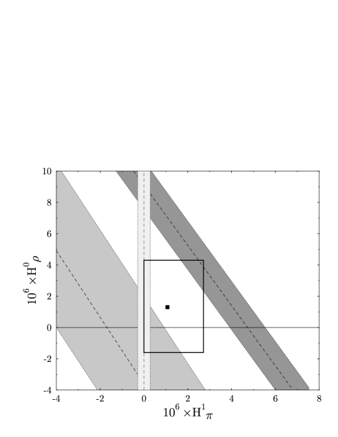
Figure 6: Weak coupling constants $H^{1}_{\pi}$ and $H^{0}_{\rho}$ extracted from ${}^{18}F$ (light band), ${}^{205}Tl$ (medium band), and ${}^{133}Cs$ (dark band) experiments. Also shown are the DDH [18] ”best” values (square) and ”reasonable range” (box)

where $g_{\pi}$ and $g_{\rho}$ are the strong coupling constants. The bands corresponding to the ${}^{205}Tl$ and ${}^{133}Cs$ data are slightly different from those extracted in Ref. [6]. There, our previous calculations [1] were used to extract the coupling constants from the anapole moment data.

Our improved calculations did not change the general situation. The coupling constants extracted from ${}^{133}Cs$ and ${}^{205}Tl$ data still look inconsistent independently on ${}^{19}F$ data. This situation eventually raises a question how reliable is the theory of nuclear anapole moment. Our calculation has been done using the random-phase approximation. There are two more calculations accounting for many-body effects [20], [21] within the shell model approach. In Ref. [21] the shell model basis used for calculation of the anapole moment of ${}^{205}Tl$ was large enough to account simultaneously both for the single-particle AM and the core polarization effects. The value obtained in Ref. [21] for the spin part of the anapole moment of ${}^{205}Tl$ is $\kappa_{s}=0.35$. Our calculation, where we use completely different quasi-particle interaction and the RPA, gives $\kappa_{s}=0.37$ for the ”best” values of the coupling constants. Such close values obtained in completely different approaches give hope for a weak model dependence of the AM, although we cannot exclude that this is just the coincidence.

The relation between effective PNC interaction constants and meson-nucleon coupling constants given by Eq.(32) is less reliable. The normalization factors $W_{\pi}$ and $W_{\rho}$ were determined by comparing matrix elements of the interaction Eq.(4) and the finite-range DDH interaction of Ref.[18] for $N-{{}^{4}He}$ scattering at low energy. Therefore, we hardly can expect them to be constant in a broad range of all bound single-particle states. In order to check the accuracy of this procedure we calculated $W_{\pi}$ as a ratio of typical matrix elements of the finite range DDH [18] interaction and the zero range interaction Eq.(4). The results are shown in Fig.7 where the normalization factor $W_{\pi}$ is plotted as a function of a single-particle energy for the proton and neutron states. The factor $W_{\pi}$ is really state dependent. Only near Fermi surface $W_{\pi}=0.16$. For the states with lower energy it becomes larger reaching the value $W_{\pi}\sim 0.4-0.5$ for $1s_{1/2}$ states.

Figure 7: Normalization factor $W_{\pi}$ as a function of bound state energy. Proton states are connected by dashes. Neutron states are connected by dots.

For this reason one should not use such a simple relation as Eq.(32) for determination of the PNC meson-nucleon coupling constants. There is an additional reason why Eq.(32) should not be used to extract the interaction constants. As it was shown in [22, 23] strong renormalization of the PNC nucleon-nucleon interaction can exist in nuclear media. As a result, the neutron PNC potential constant $g_{n}$ (which is small when estimated using Eq.(32)) can be comparable to the proton constant $g_{p}$. (See also discussion of the subject in Ref.[24].) From this point of view, the measurements sensitive to $g_{n}$ would be extremely interesting. These could be the measurements of the anapole moment of a nucleus with an odd neutron or, another possibility, the measurement of the neutron spin rotation in helium [10].

In order to obtain the measured value of the AM of ${}^{133}Cs$ the PNC interaction constants Eq.(5) should be increased approximately by a factor of 2 as compared to their Eq.(32) ”best values”. It is interesting to note that a similar conclusion has been obtained from statistical analysis of the PNC effects in compound nuclei [25].

In Table 3 we show the summarized results for a set of the proton odd and the neutron odd nuclei. Here we list just the sum of all contributions. For Ba isotopes the calculations were performed including the pairing. It is worth noting that for nuclei with an odd neutron due to the core polarization some contribution proportional to the proton coupling $g_{p}$ appears in the anapole moment. In case of small $g_{n}$ it can be of the same order as the direct $g_{n}$ contribution.

Table 1: Contributions to the anapole moment of ${}^{133}Cs$

$\kappa\times 10^{2}$	s.p.	$V-V_{0}$	$\delta V$	Total
		$-3.6g_{p}$	$2.5g_{p}+0.41g_{n}$	$5.9g_{p}+0.41g_{n}$	I
$\kappa_{s}\times 10^{2}$	$7.0g_{p}$		$1.2g_{p}+0.24g_{n}$	$4.6g_{p}+0.24g_{n}$	II
		$-3.5g_{p}$	$1.9g_{p}+0.17g_{n}$	$5.4g_{p}+0.17g_{n}$	III
		$0.8g_{p}$	$-0.4g_{p}-0.03g_{n}$	$-1.2g_{p}-0.03g_{n}$	I
$\kappa_{ls}\times 10^{2}$	$-1.6g_{p}$		$-0.3g_{p}-0.02g_{n}$	$-1.0g_{p}-0.02g_{n}$	II
		$0.8g_{p}$	$-0.4g_{p}-0.02g_{n}$	$-1.2g_{p}-0.02g_{n}$	III
		$-0.6g_{p}$	$0.9g_{p}+0.07g_{n}$	$-0.2g_{p}+0.07g_{n}$	I
$\kappa_{conv}\times 10^{2}$	$-0.5g_{p}$		$0.2g_{p}+0.04g_{n}$	$-0.9g_{p}+0.04g_{n}$	II
		$-0.7g_{p}$	$-0.1g_{p}+0.02g_{n}$	$-1.3g_{p}+0.02g_{n}$	III
$\kappa_{c}\times 10^{2}$	$0.65g_{pn}$			$0.45g_{pn}-0.03g_{np}$	I,II
				$0.36g_{pn}-0.02g_{np}$	III
		$-3.4g_{p}$	$2.9g_{p}+0.45g_{n}$	$4.4g_{p}+0.45g_{n}+\kappa_{c}$	I
$\kappa_{tot}\times 10^{2}$	$4.9g_{p}$		$1.1g_{p}+0.25g_{n}$	$2.7g_{p}+0.25g_{n}+\kappa_{c}$	II
	$+\kappa_{c}^{s.p.}$	$-3.4g_{p}$	$1.5g_{p}+0.18g_{n}$	$2.9g_{p}+0.18g_{n}+\kappa_{c}$	III

Table 2: Contributions to the anapole moment of ${}^{205}Tl$

$\kappa\times 10^{2}$	s.p.	$V-V_{0}$	$\delta V$	Total
$\kappa_{s}$	$10.8g_{p}$	$-5.7g_{p}$	$4.8g_{p}+0.14g_{n}$	$9.9g_{p}+0.14g_{n}$	I
$\times 10^{2}$			$3.1g_{p}+0.02g_{n}$	$8.3g_{p}+0.02g_{n}$	II
$\kappa_{ls}$	$-2.2g_{p}$	$1.1g_{p}$	$-1.0g_{p}-0.01g_{n}$	$-2.0g_{p}-0.01g_{n}$	I
$\times 10^{2}$			$-0.7g_{p}-0.01g_{n}$	$-1.8g_{p}-0.01g_{n}$	II
$\kappa_{conv}$	$-0.7g_{p}$	$-0.9g_{p}$	$0.9g_{p}+0.23g_{n}$	$-0.8g_{p}+0.23g_{n}$	I
$\times 10^{2}$			$-0.6g_{p}+0.10g_{n}$	$-2.2g_{p}+0.10g_{n}$	II
$\kappa_{c}\times 10^{2}$	$0.85g_{pn}$			$0.64g_{pn}-0.06g_{np}$	I,II
$\kappa_{tot}$	$7.8g_{p}$	$-5.5g_{p}$	$4.7g_{p}+0.35g_{n}$	$7.1g_{p}+0.35g_{n}+\kappa_{c}$	I
$\times 10^{2}$	$+\kappa_{c}^{s.p.}$		$1.9g_{p}+0.1g_{n}$	$4.3g_{p}+0.1g_{n}+\kappa_{c}$	II

Table 3: Calculated anapole moments for the set of nuclei

Nuclei	$\kappa_{s.p.}\times 10^{2}$	$\kappa\times 10^{2}$
Odd proton nuclei
133Cs	$4.9g_{p}+0.65g_{pn}$	$2.9g_{p}+0.18g_{n}+0.36g_{pn}-0.02g_{np}$
205Tl	$7.8g_{p}+0.85g_{pn}$	$4.3g_{p}+0.1g_{n}+0.64g_{pn}-0.06g_{np}$
209Bi	$5.4g_{p}+0.96g_{pn}$	$2.5g_{p}+0.3g_{n}+0.57g_{pn}-0.04g_{np}$
Odd neutron nuclei
135Ba	$-6.5g_{n}-0.25g_{np}$	$-0.1g_{p}-4.6g_{n}+0.01g_{pn}-0.19g_{np}$
137Ba	$-6.5g_{n}-0.25g_{np}$	$-0.2g_{p}-5.7g_{n}+0.01g_{pn}-0.23g_{np}$
207Pb	$-9.6g_{n}-0.16g_{np}$	$-0.1g_{p}-6.7g_{n}+0.01g_{pn}-0.14g_{np}$

References

- [1] V.F. Dmitriev, V.B. Telitsin, Nucl. Phys.A 613 (1997) 237.
- [2] C.S. Wood et al., Science 275 (1997) 1759.
- [3] W.C. Haxton, Science 275 (1997) 1753.
- [4] V.V. Flambaum and D.W. Murray, Phys. Rev. C56 (1997) 1641.
- [5] E.G. Adelberger and W.C. Haxton, Ann. Rev. Nucl. Part. Sci. 35 (1985) 501.
- [6] W.S. Wilburn and J.D. Bowman, Phys. Rev. C57 (1998) 3425.
- [7] P.A. Vetter, D.M. Meekhof, P.K. Majumder, S.K. Lamoreaux, and E.N. Fortson, Phys. Rev. Lett. 74 (1995) 2658.
- [8] V.F. Dmitriev, I.B. Khriplovich and V.B. Telitsin, Nucl. Phys. A577 (1994) 691.
- [9] V.V. Flambaum and I.B. Khriplovich, Zh. Eksp. Teor. Fiz. 79 (1980) 1656.
- [10] V.F. Dmitriev, V.V. Flambaum, O.P. Sushkov, and V.B. Telitsin, Phys. Lett. B125 (1983) 1.
- [11] V.V. Flambaum, I.B. Khriplovich, and O.P. Sushkov, Phys. Lett. B146 (1984) 367.
- [12] V.V. Flambaum, O.P. Sushkov, and V.B. Telitsin, Nucl. Phys. A 444 (1985) 611.
- [13] V.V. Flambaum, I.B. Khriplovich and O.P. Sushkov, Nucl. Phys. A 449 (1986) 750.
- [14] I.B.Khriplovich, Parity nonconservation in atomic phenomena (Gordon and Breach, London, 1991)
- [15] A.P. Platonov, E.E. Saperstein, Nucl. Phys. A486 (1988) 63.
- [16] E.E. Saperstein, M.A. Troitsky, Yadernaja Fizika 1 (1965) 400.
- [17] L.A. Malov, V.G. Soloviev, and I.D. Khristov, Yadernaja Fizika 6 (1967) 1186.
- [18] B. Desplanques, J.F. Donoghue and B.R. Holstein, Ann. Phys. 124 (1979) 449.
- [19] O.P. Sushkov and V.B. Telitsin, Phys. Rev. C 48 (1993) 1069.
- [20] W.C. Haxton, E.M. Henley, and M.J. Musolf, Phys. Rev. Lett. 63 (1989) 949.
- [21] N. Auerbach and B.A. Brown, Phys. Rev. C 60 (1999) 025501.
- [22] V.V. Flambaum, O.K. Vorov, Phys. Rev. C 49 (1994) 1827.
- [23] V.V. Flambaum and G.F. Gribakin, Prog. in Part. and Nucl. Phys., 35 (1995).
- [24] B. Desplanques, Phys. Rep. 297 (1998) 1.
- [25] S. Tomsovic, Mikkel B. Johnson, A. Hayes, and J.D. Bowman, preprint nucl-th/9911057.