Selected nucleon form factors and a composite scalar diquark

I Introduction

Current generation experiments probe hadrons and their interactions on a truly dynamical domain where symmetries alone are insufficient to characterise them. In this domain phenomenologically accurate nucleon-nucleon potentials[1, 2] and meson exchange models[3] are keys in the interpretation of data. These models are tools via which the correlated quark exchange underlying hadron-hadron interactions is realised as a sum of exchanges of elementary, meson-like degrees of freedom, and their definition relies on meson-nucleon form factors that sensibly provide short-range cutoffs in the integrals that arise in calculations.

These form factors are interpreted as a manifestation of the hadrons’ internal structure. If this interpretation is realistic then they should be calculable in models that reliably describe hadron structure. This cannot mean that models of hadron structure should exactly reproduce the momentum-dependence and parameter values used in potential models. In order to be phenomenologically successful, all models have hidden degrees of freedom, which make complicated a direct comparison between approaches. However, one can expect semi-quantitative agreement, with large discrepancies being harbingers of model artefacts and defects.

An additional complication is that the mesons of the strong interaction spectrum are bound states and hence are only unambiguously defined on-shell; i.e., at their pole position in a n-point vertex function. Any reference to an off-shell meson is necessarily model dependent. Therefore the only comparisons that can be model-independent are those between calculated meson-baryon coupling constants and on-shell couplings inferred from potential models because these comparisons do not involve the ad hoc definition of an off-shell bound state.

Primarily for this reason, the comparison between calculated and phenomenological form factors can only be qualitative and should employ more than one off-shell extrapolation to provide reliable information. In spite of the ambiguities, however, the calculation of meson-baryon form factors is an essential element of contemporary phenomenology. For example, it can expose difficulties in phenomenological interpretations, as is well exemplified by the discussion of $\rho^{0}$-$\omega$ mixing and its contribution to charge symmetry breaking in $NN$ potentials[4], and also provide guidance in constraining meson exchange currents in light nuclear systems[6, 7].

The dominant meson-like degrees of freedom employed in potential models are identified with the $\pi$, $\rho$, $\omega$ and a light scalar, $\sigma$. Herein we calculate the associated meson-nucleon coupling constants and form factors using a covariant nucleon model[8]. It is motivated by quark-diquark solutions of a relativistic Fadde’ev equation[9, 10, 11] and while only retaining a scalar diquark correlation is a limitation, the model’s treatment of that as a nonpointlike, confined composite is a significant beneficial feature. That is illustrated in its application to the calculation of nucleon electromagnetic form factors[8], which semi-quantitatively describes the ratio $\mu_{p}G_{E}^{p}(q^{2})/G_{M}^{p}(q^{2})$ recently observed at TJNAF[12]. In Sec. II we review the model. Our results are described in the next four sections: Sec. III, $\pi NN$; Sec. IV, $\omega NN$- and $\rho NN$-like interactions; Sec. V explores the nucleon’s axial-vector current; and Sec. VI focuses on the scalar-nucleon interaction. Sec. VII is a brief recapitulation and an appendix contains selected formulae.

II Nucleon Model

We represent the nucleon as a three-quark bound state involving a nonpointlike diquark correlation and write its Fadde’ev amplitude as

$$\Psi^{\tau}_{\alpha}(p_{1},\alpha_{1},\tau^{1};p_{2},\alpha_{2},\tau^{2};p_{3},\alpha_{3},\tau^{3})=$$ (2)

$$\varepsilon_{c_{1}c_{2}c_{3}}\,\delta^{\tau\tau^{3}}\,\delta_{\alpha\alpha_{3}}\,\psi(p_{1}+p_{2},p_{3})\,\Delta(p_{1}+p_{2})\,\Gamma_{\alpha_{1}\alpha_{2}}^{\tau^{1}\tau^{2}}(p_{1},p_{2})\,,$$

where $\varepsilon_{c_{1}c_{2}c_{3}}$ effects a singlet coupling of the quarks’ colour indices, $(p_{i},\alpha_{i},\tau^{i})$ denote the momentum and the Dirac and isospin indices for the $i$-th quark constituent, $\alpha$ and $\tau$ are these indices for the nucleon itself, $\psi(\ell_{1},\ell_{2})$ is a Bethe-Salpeter-like amplitude characterising the relative-momentum dependence of the correlation between diquark and quark, $\Delta(K)$ describes the propagation characteristics of the diquark, and

$$\Gamma_{\alpha_{1}\alpha_{2}}^{\tau^{1}\tau^{2}}(p_{1},p_{2}) = (Ci\gamma_{5})_{\alpha_{1}\alpha_{2}}\,(i\tau_{2})^{\tau^{1}\tau^{2}}\,\Gamma(p_{1},p_{2})$$ (3)

represents the momentum-dependence, and spin and isospin character of the diquark correlation; i.e., it corresponds to a Bethe-Salpeter-like amplitude for the diquark. While complete antisymmetrisation is not explicit in $\Psi$, it is exhibited in our calculations via the exchange of roles between the dormant and diquark-participant quarks, and gives rise to diquark “breakup” contributions to the form factors. This in not an afterthought, it merely reflects the simple manner in which we choose to order and elucidate our calculations.

With the form of $\Psi$ in Eq. (2), we retain in the quark-quark scattering matrix only the contribution of the scalar diquark, which has the largest correlation length [13]: $\lambda_{0^{+}}:=1/m_{0^{+}}=0.27\,$fm. We saw as anticipated in Ref. [8] that the primary defect of Eq. (2) is the omission of the axial-vector correlation ($\lambda_{1^{+}}\approx 0.8\,\lambda_{0^{+}}$). Nevertheless the Ansatz yielded much about the electromagnetic nucleon form factors that was quantitatively reliable and qualitatively informative. Hence, we employ it again herein as an exploratory, intuition building tool.

The amplitude in Eq. (2) is fully determined with the specification of the scalar functions:

$$\psi(\ell_{1},\ell_{2}) = \frac{1}{{\cal N}_{\Psi}}\,{\cal F}(\ell^{2}/\omega_{\psi}^{2})\,,\;\ell:=\frac{1}{3}\,\ell_{1}-\frac{2}{3}\,\ell_{2}\,,$$ (4)

$$\Gamma(q_{1},q_{2}) = \frac{1}{{\cal N}_{\Gamma}}\,{\cal F}(q^{2}/\omega_{\Gamma}^{2})\,,\;q:=\frac{1}{2}\,q_{1}-\frac{1}{2}\,q_{2}\,,$$ (5)

$$\Delta(K) = \frac{1}{m_{\Delta}^{2}}\,{\cal F}(K^{2}/\omega_{\Gamma}^{2})\,,$$ (6)

$${\cal F}(y) = \frac{1-{\rm e}^{-y}}{y}\,,$$ (7)

which introduces three parameters whose values were determined[8] in a least-squares fit to $G^{p}_{E}(q^{2})$

$$\begin{array}[]{ccc}\;\omega_{\psi}&\omega_{\Gamma}&m_{\Delta}\\ \hline\cr\;0.20&1.4&0.63\end{array}$$ (8)

all in GeV ($1/m_{\Delta}=0.31\,$fm). ${\cal N}_{\Psi}$ and ${\cal N}_{\Gamma}$ are the calculated nucleon and $(ud)$ diquark normalisation constants, which via the canonical definition ensure composite electric charges of $1$ for the proton and $1/3$ for the diquark. Current conservation is manifest in this model.

An essential, additional element in the calculation of the electromagnetic nucleon form factors is the dressed-quark propagator:

$$S(p) = -i\gamma\cdot p\,\sigma_{V}(p^{2})+\sigma_{S}(p^{2})$$ (9)

$$= \left[i\gamma\cdot p\,A(p^{2})+B(p^{2})\right]^{-1}\,.$$ (10)

While $S(p)$ can be obtained as a solution of the quark Dyson-Schwinger equation (DSE)[14], a phenomenologically efficacious algebraic parametrisation has been determined in extensive studies of meson properties[15, 16] and we employ it herein:

$$\bar{\sigma}_{S}(x) = 2\,\bar{m}\,{\cal F}(2(x+\bar{m}^{2}))$$ (12)

$$+{\cal F}(b_{1}x)\,{\cal F}(b_{3}x)\,\left[b_{0}+b_{2}{\cal F}(\epsilon x)\right]\,,$$

$$\bar{\sigma}_{V}(x) = \frac{1}{x+\bar{m}^{2}}\,\left[1-{\cal F}(2(x+\bar{m}^{2}))\right]\,,$$ (13)

$x=p^{2}/\lambda^{2}$, $\bar{m}$ = $m/\lambda$, $\bar{\sigma}_{S}(x)=\lambda\,\sigma_{S}(p^{2})$ and $\bar{\sigma}_{V}(x)=\lambda^{2}\,\sigma_{V}(p^{2})$. The mass-scale, $\lambda=0.566\,$GeV, and parameter values

$$\begin{array}[]{ccccc}\bar{m}&b_{0}&b_{1}&b_{2}&b_{3}\\ \hline\cr 0.00897&0.131&2.90&0.603&0.185\end{array}\;,$$ (14)

were fixed in a least-squares fit to light-meson observables[15]. ($\epsilon=10^{-4}$ in (12) acts only to decouple the large- and intermediate-$p^{2}$ domains.) This algebraic parametrisation combines the effects of confinement and dynamical chiral symmetry breaking with free-particle behaviour at large spacelike $p^{2}$ [16].

III Pion Nucleon Coupling

The pion-nucleon current is

$$J_{\pi}^{j}(P^{\prime},P) = \bar{u}(P^{\prime})\,\Lambda_{\pi}^{j}(q,P)\,u(P)$$ (15)

$$=: g_{\pi NN}(q^{2})\,\bar{u}(P^{\prime})\,i\tau^{j}\gamma_{5}\,u(P)\,,$$ (16)

where the spinors satisfy:

$$\gamma\cdot P\,u(P)=iMu(P)\,,\;\bar{u}(P)\,\gamma\cdot P=iM\bar{u}(P)$$ (17)

with the nucleon mass $M=0.94\,$GeV and $q=(P^{\prime}-P)$.

For an on-shell pion a calculation of the impulse approximation to $J_{\pi}^{j}$ requires only one additional element: $\Gamma^{j}_{\pi}(k;Q)$, the pion Bethe-Salpeter amplitude, with $k$ the relative quark-antiquark momentum and $Q$ the total momentum of the bound state. It has the general form

$$\Gamma_{\pi}^{j}(k;Q) = \tau^{j}\gamma_{5}\left[iE_{\pi}(k;Q)+\gamma\cdot Q\,F_{\pi}(k;Q)\rule{0.0pt}{14.22636pt}\right.$$ (18)

$$+ \left.\rule{0.0pt}{14.22636pt}\gamma\cdot k\,k\cdot Q\,G_{\pi}(k;Q)+\sigma_{\mu\nu}\,k_{\mu}Q_{\nu}\,H_{\pi}(k;Q)\right]$$ (19)

and is obtained as a solution of an homogeneous Bethe-Salpeter equation.

Using any truncation of the quark-antiquark scattering matrix that ensures the preservation of the axial-vector Ward-Takahashi identity then, in the chiral limit[17],

$$E_{\pi}(k;Q=0) = \frac{1}{f_{\pi}}B_{0}(k^{2})\,,$$ (20)

and $F_{\pi}$, $G_{\pi}$, $H_{\pi}$ satisfy similar relations involving $A_{0}(k^{2})$. Here $f_{\pi}$ is the pion decay constant and $A_{0}(k^{2})$, $B_{0}(k^{2})$ are the dressed-quark propagator functions in Eq. (10) calculated in the chiral limit. Since[14, 16]

$$A(p^{2})\neq 1\,,$$ (21)

the identities involving $F_{\pi}$, $G_{\pi}$, $H_{\pi}$ entail that the pion necessarily has pseudovector components, even in the chiral limit. These components are crucial at large pion energy; e.g., they are responsible for the asymptotic $1/q^{2}$-behaviour of the electromagnetic pion form factor[18], however, for pion energy $\mathrel{\hbox to0.0pt{\lower 4.0pt\hbox{\hskip 0.0pt$\sim$}\hss}\raise 1.0pt\hbox{$<$}}1\,$GeV they are quantitatively unimportant, and Eq. (18) with Eq. (20) and $F_{\pi}=0=G_{\pi}=H_{\pi}$ provides a reliable approximation.

This fact is useful in phenomenological applications, and away from the chiral limit an algebraic parametrisation has been developed[15, 19] to be used in concert with Eqs. (12,13):

$$E_{\pi}(k;Q)=\frac{1}{f_{\pi}}\,B_{\pi}(k^{2})\,,$$ (22)

where $B_{\pi}(k^{2})$ is obtained from Eqs. (10-13) with[20]

$$\bar{m}\to 0\,,\;b_{0}\to b_{0}^{\pi}=0.204\,.$$ (23)

This form of dressed-quark propagator and pion Bethe-Salpeter amplitude yields (quoted with GeV as the base unit)

$$\begin{array}[]{l|cccc}&f_{\pi}&m_{\pi}&\langle\bar{q}q\rangle^{1\,{\rm GeV}^{2}}_{0}&\langle\bar{q}q\rangle^{1\,{\rm GeV}^{2}}_{\pi}\\ \hline\cr{\rm Calc.}&0.0924&0.141&(0.221)^{3}&(0.257)^{3}\\ {\rm Obs.\cite[cite]{[\@@bibref{Number}{pdg,mr97}{}{}]}}&0.0924&0.138&(0.241)^{3}&(0.245)^{3}\end{array}$$ (24)

The (on-shell) Bethe-Salpeter amplitude is sufficient to calculate the pion-nucleon coupling. However, to calculate the form factor we must specify an off-shell extrapolation of $E_{\pi}(k;Q)$; i.e., a functional dependence for $Q^{2}\neq-m_{\pi}^{2}$. Two obvious Ansätze are

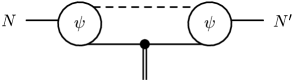
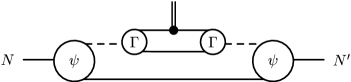
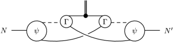
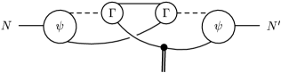
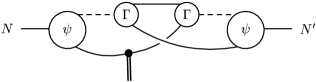
FIG. 1.: Our impulse approximation to the meson-nucleon form factors requires the calculation of five contributions, which differ in detail for each probe. $\psi$: $\psi(\ell_{1},\ell_{2})$ in (4); $\Gamma$: Bethe-Salpeter-like diquark amplitude in (3); dashed line: $\Delta(K)$, diquark propagator in (6); solid internal line: $S(q)$, quark propagator in (9); and double-line: meson-like probe. The lowest three diagrams, which describe the interchange between the dormant quark and the diquark participants, effect the antisymmetrisation of the nucleon’s Fadde’ev amplitude.

$${\rm a)}\;\;f_{\pi}\tilde{E}_{\pi}(k;Q) = B_{\pi}(k^{2})\,,$$ (25)

$${\rm b)}\;\;f_{\pi}\tilde{E}_{\pi}(k;Q) = \frac{1}{2}\left[B_{\pi}(k_{+}^{2})+B_{\pi}(k_{-}^{2})\right]\,,$$ (26)

with $k_{\pm}=k\pm Q/2$. The first, which assumes no change off shell, has been used with phenomenological success in a variety of calculations that explore meson-loop corrections to hadronic observables[23]; the second[14] allows some minimal dependence on $k\cdot Q$, $Q^{2}$; and for $Q=0$ both satisfy the constraint of Eq. (22) [cf. Eq. (20)].

As with the electromagnetic form factors, five distinct diagrams contribute to the nucleon form factors, which are depicted in Fig. 1. For the $\pi NN$ coupling these diagrams, enumerated from top to bottom, are mnemonics for the vertices $\Lambda_{\pi}^{nj}(q,P)$ given in Eqs. (101-108). As can be anticipated, $\Lambda_{\pi}^{2j}(q,P)\equiv 0$ because of parity conservation; i.e., a Poincaré invariant theory can’t admit a three-point pseudoscalar-scalar-scalar coupling.

The pion-nucleon vertex:

$$\Lambda^{j}_{\pi}(q,P)=\Lambda^{1j}_{\pi}(q,P)+2\sum_{n=2}^{5}\,\Lambda^{nj}_{\pi}(q,P)\,,$$ (27)

is completely expressed in terms of four independent scalar functions

$$\Lambda_{\pi}^{j}(q,P)=\tau^{j}\gamma_{5}\left[\,if_{1}+\gamma\cdot q\,f_{2}+\gamma\cdot R\,f_{3}+\sigma_{\mu\nu}R_{\mu}q_{\nu}\,f_{4}\right]$$ (28)

where $f_{i}=f_{i}(q^{2})$, $R=(P^{\prime}+P)$ and $q\cdot R=0$ for nucleon elastic scattering. From this we construct the pion-nucleon current

$$J_{\pi}^{j}(P^{\prime},P)=\bar{u}(P^{\prime})\,\Lambda_{\pi}^{j}(q,P)\,u(P)\,,$$ (29)

and employing the definition of the nucleon spinors, Eqs. (17), we identify the pion-nucleon coupling in Eq. (15):

$$g_{\pi NN}(q^{2}) = f_{1}-2\,M\,f_{2}+R^{2}\,f_{4}\,.$$ (30)

TABLE I.: Calculated couplings compared with: contemporary meson exchange model values[3], where available; experiment in the case of $g_{A}$, $r_{A}$[24]; a lattice-QCD result for $\sigma$[25]; and for $g_{\sigma}$, $r_{\sigma}$, as discussed in connection with Eqs. (96-99). Also for comparison, the pion model described in Sec. II yields[15] $r_{\pi}=0.56\,$fm. The labels “a)” etc. identify the results obtained with: Eqs. (25,26) for $\pi NN$; Eqs. (45,46,48) for $VNN$; and Eqs. (70,71) for the axial-vector coupling.

$\displaystyle\begin{array}[]{l|ccc}&{\rm Calc.}&{\rm Estimates}&{\rm Expt.}\\ \hline\cr g_{\pi NN}&~{}14.9&13.4&\\ \hline\cr\langle r_{\pi NN}^{2}\rangle^{1/2}&\begin{array}[]{l}a)\;0.71\\ b)\;0.80\end{array}&0.93-1.06\,{\rm fm}&\\ \hline\cr g_{\rho NN}&\begin{array}[]{l}a)\;5.92\\ b)\;6.26\\ c)\;4.82\end{array}&6.4&\\ \hline\cr f_{\rho NN}&\begin{array}[]{l}a)\;15.4\\ b)\;16.6\\ c)\;12.6\end{array}&13.0&\\ \hline\cr\kappa_{\rho}&\begin{array}[]{l}a)\;2.57\\ b)\;2.64\\ c)\;2.61\end{array}&2.0&\\ \hline\cr g_{\omega NN}&\begin{array}[]{l}a)\;9.74\\ b)\;10.2\\ c)\;11.5\end{array}&7-10.5&\\ \hline\cr f_{\omega NN}&\begin{array}[]{l}a)\;9.62\\ b)\;10.7\\ c)\;4.39\end{array}&&\\ \hline\cr\kappa_{\omega}&\begin{array}[]{l}a)\;0.99\\ b)\;1.04\\ c)\;0.38\end{array}&&\\ \hline\cr g_{A}&\begin{array}[]{l}a)\;0.80\\ b)\;0.99\end{array}&&1.259\pm 0.017\\ \hline\cr\langle r_{A}^{2}\rangle^{1/2}&\begin{array}[]{l}a)\;0.75\\ b)\;0.75\end{array}&&0.68\pm 0.12\,{\rm fm}\\ \hline\cr\sigma/M_{N}&~{}0.015&0.019\pm 0.05&\\ \hline\cr g_{\sigma}&9.3&10\\ \hline\cr\langle r_{\sigma NN}^{2}\rangle^{1/2}&~{}0.89&1.2\,{\rm fm}&\\ \hline\cr\end{array}$

FIG. 2.: Calculated pion-nucleon form factor, compared with dipole fits, Eqs. (31,32).

Using Monte-Carlo methods to evaluate the integrals we obtain the coupling, $g_{\pi NN}:=g_{\pi NN}(q^{2}=0)$, in Table I. It is 11% too large. (Our statistical error is always $<1\,$%.) We anticipate that retaining pseudovector components in $\Gamma_{\pi}^{j}(k;Q)$ and an axial-vector diquark correlation will only slightly affect this value as long as they are constrained consistently with the model. An ad hoc addition of the pseudovector components can have large effects[26].

The relative strength of the contribution from each diagram in Fig. 1 is presented in Table II. We observe that the diquark breakup terms are just as important here as they were in the calculation of the nucleon charge radii and magnetic moments[8]. These diagrams are the true measure of the diquark’s composite nature, which is not captured by simply adding a diquark “vertex function.”

TABLE II.: Relative contribution to the couplings of each of the terms represented mnemonically by the five diagrams in Fig. 1. In building this table we used the amplitudes in Eq. (25) for the $\pi$, Eqs. (45,48) for the vector couplings, and the dressed-quark-axial-vector vertex of Eqs. (67,71). In all cases the crucial role of the diquark breakup diagrams is evident. Diagram 2 will contribute to all processes if an axial-vector diquark correlation is included.

$\displaystyle\begin{array}[]{lr|rrrrr}&{\rm diagram}&1&2&3&4&5\\ \hline\cr g_{\pi NN}&&0.65&0.00&0.07&0.14&0.14\\ g_{\rho NN}&{\rm a)}&0.74&0.00&-0.06&0.16&0.16\\ &{\rm c)}&0.73&0.00&-0.11&0.19&0.19\\ f_{\rho NN}&{\rm a)}&0.64&0.00&0.10&0.13&0.13\\ &{\rm c)}&0.64&0.00&0.12&0.12&0.12\\ g_{\omega NN}&{\rm a)}&0.45&0.31&0.04&0.10&0.10\\ &{\rm c)}&0.31&0.49&0.05&0.08&0.08\\ f_{\omega NN}&{\rm a)}&1.04&-0.28&-0.16&0.20&0.20\\ &{\rm c)}&1.81&-1.16&-0.35&0.35&0.35\\ g_{A}&&0.63&0.00&0.09&0.14&0.14\\ \sigma&&0.58&0.19&0.03&0.10&0.10\end{array}$

The $\pi NN$ form factor calculated using both off-shell Ansätze, Eqs. (25,26), is plotted in Fig. 2. We have performed monopole and dipole fits to our calculated result:

$$g_{\pi NN}(q^{2})=\frac{g_{\pi NN}}{(1+q^{2}/\Lambda_{\pi}^{2})^{n}}\,,\;n=1,2\,,$$ (31)

and obtain pole masses, in GeV,

$$\begin{array}[]{l|cc}&n=1&n=2\\ \hline\cr{\rm Eq.~{}(\ref{GaPia})}&0.63&0.96\\ {\rm Eq.~{}(\ref{GaPib})}&0.57&0.85\end{array}\,.$$ (32)

The dipole form provides an accurate interpolation on the entire range shown. However, the monopole form is only accurate for $q^{2}\mathrel{\hbox to0.0pt{\lower 4.0pt\hbox{\hskip 0.0pt$\sim$}\hss}\raise 1.0pt\hbox{$<$}}0.4\,$GeV², overestimating the result by $\sim 70\,$% at $q^{2}=3.0\,$GeV². (Requiring that the fits are accurate in the neighbourhood of $q^{2}=0$ ensures $\Lambda_{\pi}^{\rm dipole}/\Lambda_{\pi}^{\rm monopole}\approx\surd 2$.) Thus our calculations favour soft form factors, in semi-quantitative agreement with those employed in Ref.[3] and advocated in Ref.[27]. We can further quantify this by introducing a pionic radius of the nucleon:

$$\langle r_{\pi NN}^{2}\rangle:=-\frac{6}{g_{\pi NN}}\,\left.\frac{dg_{\pi NN}(q^{2})}{dq^{2}}\right|_{q^{2}=0}\,.$$ (33)

Our calculated value is presented in Table I and can be compared with the analogous tabulated quantities. It is almost three-times larger than $r_{\pi NN}\sim 0.3\,$fm inferred from Ref. [1].

IV Vector-meson Nucleon Coupling

In this section we consider $\omega$-$NN$- and $\rho$-$NN$-like interactions; i.e., isoscalar-vector and isovector-vector couplings. The vector-meson–nucleon current is

$$J_{\mu}^{V\alpha}(P^{\prime},P)=$$ (35)

$$i\,\bar{u}(P^{\prime})\frac{\tau^{\alpha}}{2}\left(\gamma_{\mu}\,F_{1}^{V}(q^{2})+\frac{1}{2M}\,\sigma_{\mu\nu}\,q_{\nu}\,F_{2}^{V}(q^{2})\right)u(P)\,,$$

with $\tau^{0}:={\rm diag}(1,1)$ and $\tau^{1,2,3}$ the usual Pauli matrices. Although the complete specification of a fermion-vector boson vertex:

$$\Lambda_{\mu}^{\alpha}(q,P):=\frac{\tau^{\alpha}}{2}\,\Lambda_{\mu}(q,P)\,,$$ (36)

requires twelve independent scalar functions,

$$i\Lambda_{\mu}(q,P)=i\gamma_{\mu}\,f_{1}+i\sigma_{\mu\nu}\,q_{\nu}\,f_{2}+R_{\mu}\,f_{3}+i\gamma\cdot R\,R_{\mu}\,f_{4}$$ (38)

$$+i\sigma_{\nu\rho}\,R_{\mu}\,q_{\nu}\,R_{\rho}\,f_{5}+i\gamma_{5}\gamma_{\nu}\,\varepsilon_{\mu\nu\rho\sigma}\,q_{\rho}\,R_{\sigma}\,f_{6}\,+\ldots\,,$$

using Eq. (17) only the six shown explicitly contribute to $F_{1,2}$:

$$F_{1}=$$ (40)

$$f_{1}+2\,M\,f_{3}-4\,M^{2}\,f_{4}-2\,M\,q^{2}\,f_{5}-q^{2}\,f_{6}\,,$$

$$F_{2}=$$ (42)

$$2\,M\,f_{2}-2\,M\,f_{3}+4\,M^{2}\,f_{4}+2\,M\,f_{5}-4\,M^{2}\,f_{6}\,.$$

The coupling strengths relevant for comparison with potential models are

$$g_{VNN}:=F_{1}^{V}(0)\,,\;f_{VNN}:=F_{2}^{V}(0)\,,\;\kappa_{V}:=\frac{f_{VNN}}{g_{VNN}}$$ (43)

because these are $t$-channel elastic scattering models. However, we note that $q^{2}=0$ is a far off-shell point for the $\omega$ and $\rho$ of the strong interaction spectrum, for which $(-q^{2})=M_{V}^{2}\approx 0.6\,$GeV². Hence a calculation of these coupling constants is only possible after an off-shell extrapolation of the vector meson Bethe-Salpeter amplitude is specified.

Quantitatively reliable numerical solutions of the vector meson Bethe-Salpeter equation have recently become available[28], however, an algebraic Ansatz compatible with our parametrisation of the dressed-quark propagator, Eqs.(12,13), is not yet available. Hence, we use Ansätze motivated by an extensive study of light- and heavy-meson observables[20]:

$$\Gamma_{\mu}^{\alpha}(k;Q)=\frac{1}{{\cal N}_{V}}\left(\gamma_{\mu}-\frac{Q_{\mu}\gamma\cdot Q}{Q^{2}}\right)\varphi(k^{2})\,\tau^{\alpha}\,,$$ (44)

$${\rm a)}\;\;\varphi(k^{2}) = 1/(1+k^{4}/\omega^{4})\,,$$ (45)

$${\rm b)}\;\;\varphi(k^{2}) = \left[{\cal F}(k^{2}/\omega^{2})\right]^{2}\,,$$ (46)

with $\omega=0.515\,$GeV and the normalisation: ${\cal N}_{V}$, determined canonically, Eq. (122). With these simple forms of $\Gamma_{\mu}^{\alpha}(k;Q)$ we obtain the following values of the electromagnetic and strong coupling constants:

$$\begin{array}[]{l|cccc}&a)&b)&c)&{\rm Obs.\cite[cite]{[\@@bibref{Number}{pdg}{}{}]}}\\ \hline\cr g_{\rho}&6.57&6.05&&5.03\pm 0.012\\ g_{\rho\pi\pi}&8.75&10.7&8.52&6.05\pm 0.02\end{array}\,,$$ (47)

results which suggest that errors of up-to 40% could arise in nucleon calculations involving these amplitudes.

The calculation of the vector-meson–nucleon current is now straightforward with $F_{1,2}$ determined by calculating the integrals in Eqs. (111-119) and combining their contributions according to Eqs. (40,42,123). In this way we obtain the couplings presented in Table I, with the relative strength of the contribution from each diagram given in Table II.

The couplings are in semi-quantitative agreement with those inferred from meson-exchange models[3] except in the case of $f_{\omega NN}$. Using Eqs. (45,46) we obtain $f_{\omega NN}\approx g_{\omega NN}$ while contemporary phenomenological models, which are only weakly sensitive to $f_{\omega NN}$, assume it to be zero. To determine the extent to which this result is model dependent we also calculate the couplings using

FIG. 3.: Calculated vector-meson–nucleon form factors. A good interpolation of the results is obtained with Eqs. (50,51).

$${\rm c)}\;\;\varphi(k^{2})=\frac{1}{{\cal N}_{V}}\,B_{V}(k^{2})\,,$$ (48)

where $B_{V}(k^{2})$ is obtained from Eqs. (10-13) with[19] $\bar{m}\to 0$ and

$$b_{0}\to b_{0}^{V}=0.044\,,\;b_{1}\to b_{1}^{V}=0.580\,,\;b_{3}\to b_{3}^{V}=0.462\,.$$ (49)

The amplitude is canonically normalised via Eq. (122) and yields $g_{\rho\pi\pi}$ in Eq. (47).

The nucleon couplings are given in Table I with the relative strength of the contribution from each diagram presented in Table II. In this case, while the other couplings change by $\mathrel{\hbox to0.0pt{\lower 4.0pt\hbox{\hskip 0.0pt$\sim$}\hss}\raise 1.0pt\hbox{$<$}}20\,$%, we find $f_{\omega^{\rm c)}NN}\approx 0.4\,g_{\omega^{\rm c)}NN}$. The reason appears in Table II: the strength of diagram 2 is much increased, and while it doesn’t contribute at all for the $\rho$ and is additive for $g_{\omega NN}$, it is a destructive contribution to $f_{\omega NN}$. This sensitivity to cancellations involving diagram 2 repeats the pattern we observed in calculating the nucleon’s isoscalar electromagnetic form factor[8] and hence $f_{\omega NN}$ is sensitive to the omission of the axial-vector diquark correlation.

The vector-meson–nucleon form factors calculated using Eq. (45) are depicted in Fig. 3 and the quadrupole

$$F_{n}^{V}(q^{2})=F_{n}^{V}(0)\,\frac{1}{(1+q^{2}/\Lambda^{V}_{n})^{3}}$$ (50)

with pole masses, in GeV,

$$\begin{array}[]{cccc}\Lambda_{1}^{\omega}&\Lambda_{2}^{\omega}&\Lambda_{1}^{\rho}&\Lambda_{2}^{\rho}\\ 1.12&1.11&1.06&1.18\end{array}$$ (51)

provides an excellent interpolation of the results. Again, these are soft form factors.

On the domain explored, our results for the $VNN$ form factor are qualitatively unaffected by employing a monopole for $\varphi(k^{2})$ in Eq. (44).

V Axial-vector Nucleon Coupling

Neutron $\beta$-decay is described by the axial-vector–nucleon current

$$J_{5\mu}^{j}(P^{\prime},P)=i\bar{u}(P^{\prime})\,\Lambda_{5\mu}^{j}(q,P)u(P)$$ (52)

$$=: i\bar{u}(P^{\prime})\,\gamma_{5}\frac{\tau^{j}}{2}\left[\gamma_{\mu}g_{A}(q^{2})+q_{\mu}g_{P}(q^{2})\right]u(P)\,,$$ (53)

which involves two form factors: $g_{A}(q^{2})$ is the axial-vector form factor of the nucleon and $g_{P}(q^{2})$ is the induced pseudoscalar form factor. The complete specification of a fermion-axial-vector vertex:

$$\Lambda_{5\mu}^{j}(q,P):=\frac{\tau^{j}}{2}\,\Lambda_{5\mu}(q,P)\,,$$ (54)

requires twelve independent scalar functions,

$$\Lambda_{5\mu}(q,P)=$$ (56)

$$\gamma_{5}\gamma_{\mu}\,f_{1}+\gamma_{5}\sigma_{\mu\nu}R_{\nu}\,f_{2}+\epsilon_{\mu\nu\rho\sigma}\,\gamma_{\nu}q_{\rho}R_{\sigma}\,f_{3}+\ldots$$

but using Eqs. (17) only the three shown explicitly contribute to the axial-vector form factor:

$$g_{A}(q^{2})=f_{1}-2Mf_{2}-q^{2}f_{3}\,.$$ (57)

In the chiral limit and in the neighbourhood of $q^{2}=0$[17, 22]

$$\Lambda_{5\mu}^{j}(q,P)={\it regular}+\frac{q_{\mu}}{q^{2}}\,f_{\pi}\,\Lambda_{\pi}^{j}(q,P)\,,$$ (58)

where $\Lambda_{\pi}^{j}(q,P)$ is the pion-fermion vertex and regular denotes non-pole terms. It follows that in this neighbourhood the induced pseudoscalar coupling is dominant and, using Eq. (15), is determined by the pion-nucleon coupling:

$$\left.q^{2}J_{5\mu}^{j}(P^{\prime},P)\right|_{q^{2}=0}$$ (59)

$$= q_{\mu}\,f_{\pi}\,g_{\pi NN}(q^{2}=0)\,\bar{u}(P^{\prime})i\tau^{j}\gamma_{5}\,u(P)$$ (60)

$$= q_{\mu}\,\bar{u}(P^{\prime})\,\gamma_{5}\frac{\tau^{j}}{2}\,[q^{2}g_{P}(q^{2})]_{q^{2}=0}\,u(P)\,.$$ (61)

Current conservation: $q_{\mu}\,J_{5\mu}^{j}(q,P)=0$, which using Eqs. (17) entails

$$-\,2Mg_{A}(q^{2}=0)+\left.\left[q^{2}\,g_{P}(q^{2})\right]\right|_{q^{2}=0}=0\,,$$ (62)

then yields the Goldberger-Treiman relation:

$$M\,g_{A}(q^{2}=0)=f_{\pi}\,g_{\pi NN}(q^{2}=0)\,.$$ (63)

This brief analysis emphasises that $g_{A}(q^{2})$ is the regular part of the axial-vector–nucleon current.

To calculate $g_{A}(q^{2})$ in impulse approximation we must specify the dressed-quark-axial-vector vertex: $\Gamma_{5\mu}^{j}(k;Q)$. It satisfies a Ward-Takahashi identity, which in the chiral limit is

$$-iQ_{\mu}\Gamma_{5\mu}^{j}(k;Q) = S^{-1}(k_{+})\gamma_{5}\frac{\tau^{j}}{2}+\gamma_{5}\frac{\tau^{j}}{2}S^{-1}(k_{-})\,.$$ (64)

This identity is solved by

$$\Gamma_{5\mu}^{j}(k;Q)=\Gamma_{5\mu}^{Rj}(k;Q)+\left[i\frac{Q_{\mu}}{Q^{2}}\,2\,\Sigma_{B}(k_{+}^{2},k_{-}^{2})\right]\,,$$ (65)

$$\Gamma_{5\mu}^{Rj}(k;Q)=\Gamma_{5\mu}^{Tj}(k;Q)$$ (66)

$$+ \gamma_{5}\frac{\tau^{j}}{2}\left(\rule{0.0pt}{15.00002pt}\gamma_{\mu}\,\Sigma_{A}(k_{+}^{2},k_{-}^{2})+2\,k_{\mu}\,\gamma\cdot k\,\Delta_{A}(k_{+}^{2},k_{-}^{2})\right)\,,$$ (67)

where $Q_{\mu}\Gamma_{5\mu}^{Tj}(k;Q)=0$ but $\Gamma_{5\mu}^{Tj}(k;Q)$ is otherwise unconstrained by the Ward-Takahashi identity and

$$\Sigma_{f}(p^{2},q^{2}) := \frac{1}{2}\,[f(p^{2})+f(q^{2})]\,,$$ (68)

$$\Delta_{f}(p^{2},q^{2}) := \frac{f(p^{2})-f(q^{2})}{p^{2}-q^{2}}\,.$$ (69)

The parenthesised term in Eq. (65) makes explicit the simple kinematic singularity associated with the pion pole. It is directly connected with the nucleon’s induced pseudoscalar form factor and, using Eqs. (20,26), clearly saturates Eq. (60). The regular part of the vertex, Eq. (67), is primarily responsible for the nucleon’s axial-vector form factor and in our calculations we complete its definition using either of two Ansätze for the transverse part:

$${\rm a})\;\;\Gamma_{5\mu}^{Tj}(k;Q) = 0\,,$$ (70)

$${\rm b})\;\;\Gamma_{5\mu}^{Tj}(k;Q) = \frac{1}{\sqrt{2}}\,\frac{f_{a_{1}}m_{a_{1}}}{Q^{2}+m_{a_{1}}^{2}}\,\Gamma_{\mu}^{a_{1}j}(k;Q)\,,$$ (71)

where $\Gamma_{\mu}^{a_{1}j}(k;Q)$ is the $a_{1}$-meson Bethe-Salpeter amplitude, which is given explicitly in Eq. (124). Model $a)$: Eqs. (67,70), is a minimal Ansatz that correctly isolates the pion pole. Model $b)$: Eqs. (67,71), is kindred to that advocated for the dressed-quark-vector vertex in Ref. [29]. It recognises that the dressed-quark-axial-vector vertex has a pole at $Q^{2}=-m_{a_{1}}^{2}$ with residue $f_{a_{1}}m_{a_{1}}$ where $f_{a_{1}}$ is the weak decay constant, and implements a model to represent the off-shell remnant of this contribution.

$g_{A}(q^{2})$ is obtained by evaluating the integrals in Eqs. (134-141) and combining their contributions according to Eqs. (57,142). The calculated coupling is presented in Table I with the relative strength of the contribution from each diagram given in Table II.

FIG. 4.: Axial-vector–nucleon form factor calculated using the Ansätze of Eqs. (70,71) compared with a monopole fit, Eqs. (72,73).

The axial-vector form factor is depicted in Fig. 4. It is important and interesting to note that the dominant, orbital $e_{2}^{a_{1}}$-term in $\Gamma_{\mu}^{a_{1}}$ contributes $<10\,$% to $g_{A}(q^{2})$ on the illustrated domain, increasing from $0$% with increasing $q^{2}$; i.e., the bulk of the difference between the $a)$ and $b)$ calculations arises from the $e_{1}^{a_{1}}$-term. In Fig. 4 we also plot a monopole fit to each calculation

$$g_{A}(q^{2})=g_{A}(0)\,\frac{1}{(1+q^{2}/\Lambda_{A}^{2})}$$ (72)

with pole masses, in GeV,

$$\begin{array}[]{l|cc}&{\rm a})&{\rm b})\\ \hline\cr\Lambda_{A}&0.65&0.64\end{array}$$ (73)

The fit provides a better representation for Ansatz $b)$ than for $a)$, and we judge $b)$ to be the more realistic model. The axial radius of the nucleon is

$$\langle r_{A}^{2}\rangle:=-\frac{6}{g_{A}(0)}\,\left.\frac{dg_{A}(q^{2})}{dq^{2}}\right|_{q^{2}=0}$$ (74)

and our calculated value is presented in Table I: $r_{A}\approx r_{\pi NN}$ in accordance with Ref. [27].

Even though our framework manifestly preserves the axial-vector Ward-Takahashi identity the model is not guaranteed to satisfy the Goldberger-Treiman relation because we employ Ansätze for the Fadde’ev amplitude and dressed-quark-axial-vector vertex that need not be mutually consistent. For example, in deriving Eq. (63) we used Eqs. (17), which introduce $M$, however, $\Psi$ in Eq. (2) is not the solution of a Fadde’ev equation with eigenvalue $M$. Indeed, without an axial-vector diquark correlation, the calculated nucleon mass is 30-50% too large[10, 34, 35]. The following comparisons (in GeV) exhibit this uncertainty:

$$\left.\begin{array}[]{l}{\rm a})\;\;Mg_{A}(0)=0.75-1.1\\ {\rm b})\;\;Mg_{A}(0)=0.93-1.4\end{array}\right\}\;\;{\rm cf.}\;\;f_{\pi}g_{\pi NN}=1.37\,.$$ (75)

and show that model Ansatz $b)$ is broadly consistent with the Goldberger-Treiman relation.

A comparison between the results obtained with the two vertex Ansätze demonstrates that a calculation of the dressed-quark-axial-vector vertex, akin to that of the dressed-quark-vector vertex in Ref. [29], would be very helpful in demarcating the importance of axial-vector diquark correlations. As shown by the model $b)$ calculation, $\Gamma_{5\mu}^{Tj}$ easily provides contributions of the same order of magnitude as that which might be anticipated from an axial-vector diquark.

VI Nucleon Sigma Term

As a final application we explore the nucleon $\sigma$-term:

$$\sigma(q^{2})\,\bar{u}(P^{\prime})u(P):=\langle P^{\prime}|\,m(\bar{u}u+\bar{d}d)\,|P\rangle\,,$$ (76)

$\sigma:=\sigma(q^{2}=0)$, which is the in-nucleon expectation value of the explicit chiral symmetry breaking term in the QCD Lagrangian. The general form for a fermion-scalar vertex is

$$\Lambda_{\mbox{\boldmath$1$}}(q,P)=f_{1}+i\gamma\cdot q\,f_{2}+i\gamma\cdot R\,f_{3}+i\sigma_{\mu\nu}R_{\mu}q_{\nu}\,f_{4}\,,$$ (77)

however, using Eqs. (17) we find

$$J_{\mbox{\boldmath$1$}}(P^{\prime},P) := \bar{u}(P^{\prime})\Lambda_{\mbox{\boldmath$1$}}(q,P)u(P)$$ (78)

$$= s(q^{2})\,\bar{u}(P^{\prime})\,u(P)\,,$$ (79)

$$s(q^{2}) = f_{1}-2Mf_{3}+q^{2}f_{4}\,.$$ (80)

To evaluate the matrix element in Eq. (76) we need the dressed-quark-scalar vertex, which is an analogue of the dressed-quark-axial-vector vertex used in Sec. V. In this case, however, there isn’t a Ward-Takahashi identity to help us. Instead, we calculate the vertex by solving an inhomogeneous Bethe-Salpeter equation using a simple, separable model for the quark-antiquark scattering kernel[13] that has been used successfully in a variety of phenomenological applications[30, 36].

The inhomogeneous vertex equation in the separable model is

$$\Gamma_{\mbox{\boldmath$1$}}(k;Q)=$$ (82)

$$\mbox{\boldmath$1$}-\frac{4}{3}\int\frac{d^{4}q}{(2\pi)^{4}}\Delta(k-q)\gamma_{\mu}S(q_{+})\Gamma_{\mbox{\boldmath$1$}}(q;Q)S(q_{-})\gamma_{\mu}\,,$$

with the interaction

$$\Delta(k-q)=G(k^{2})G(q^{2})+k\cdot q\,F(k^{2})G(k^{2})\,,$$ (83)

where

$$F(k^{2})=\frac{1}{a}[A(k^{2})-1]\hskip 14.22636ptG(k^{2})=\frac{1}{b}[B(k^{2})-\tilde{m}]\,,$$ (84)

$a=\bar{a}\lambda^{2}$, $b=\bar{b}\lambda^{2}$, and $A(k^{2})$, $B(k^{2})$ are obtained in the usual way from Eqs. (128,129) with $\tilde{m}=\hat{m}\lambda$ and $b_{2}^{a_{1}}\to b_{2}$. The separable model was constrained to fit $\pi$ and $K$ properties, as discussed in detail in Ref. [13].

Using this model the most general form of the scalar vertex is

$$\Gamma_{\mbox{\boldmath$1$}}(k;Q)=\mbox{\boldmath$1$}\,g_{1}+ik\cdot Q\gamma\cdot Q\,g_{2}+i\gamma\cdot k\,g_{3}\,,$$ (85)

where $g_{i}=g_{i}(k;Q)$. Substituting Eq. (85) in Eq. (82) we obtain the solution

$$\Gamma_{\mbox{\boldmath$1$}}(k;Q)=\mbox{\boldmath$1$}+t_{1}(Q^{2})\,G(k^{2})$$ (87)

$$+\,i\,t_{2}(Q^{2})\,F(k^{2})\frac{k\cdot Q\,\gamma\cdot Q}{Q^{2}}+\,i\,t_{3}(Q^{2})F(k^{2})\gamma\cdot k\,,$$

with $t_{i}(Q^{2})$ determined functions of their argument.

The $\sigma$-term is only sensitive to the vertex at $Q^{2}=0$, where the explicit form of the solution reduces to

$$\Gamma_{\mbox{\boldmath$1$}}(k;Q)|_{Q^{2}=0}=\mbox{\boldmath$1$}+t_{1}(0)\,G(k^{2})+t_{3}(0)\,F(k^{2})\,i\gamma\cdot k\,,$$ (88)

with $t_{1}(0)=0.242\,$GeV, $t_{3}(0)=-0.0140\,$GeV. It is important to note from Eqs. (84,88) that the $t_{1}$-term contributes $1.4\times(B(k^{2})-\tilde{m})/\sqrt{b}$ so that at $k^{2}=0$ it is 6-times larger than the bare term; i.e., it is dominant in the infrared. That is to be expected because it represents the effect of the nonperturbative dynamical chiral symmetry breaking mechanism in the solution. This and the other $g_{i}$-terms vanish as $k^{2}\to\infty$, which is a manifestation of asymptotic freedom in the separable model.

The vertex equation has a solution for all $Q^{2}$, and that solution exhibits a pole at the $\sigma$-meson mass; i.e., in the neighbourhood of $(-Q^{2})=m_{\sigma}^{2}=(0.715\,{\rm GeV})^{2}$

$$\Gamma_{\mbox{\boldmath$1$}}(k;Q)={\it regular}\;+\frac{n_{\sigma}m_{\sigma}^{2}}{Q^{2}+m_{\sigma}^{2}}\,\Gamma_{\sigma}(k;Q)\,,$$ (89)

where regular indicates terms that are regular in this neighbourhood and $\Gamma_{\sigma}(k;Q)$ is the canonically normalised $\sigma$-meson Bethe-Salpeter amplitude, whose form is exactly that of $(\Gamma_{\mbox{\boldmath$1$}}(k;Q)-\mbox{\boldmath$1$})$ in Eq. (87). The simple pole appears in the functions $t_{i}(Q^{2})$ and performing a pole fit we find

$$m\,n_{\sigma}=3.3\,{\rm MeV}\,.$$ (90)

$n_{\sigma}m_{\sigma}^{2}$ is the analogue of the residue of the pion pole in the pseudoscalar vertex[17, 22]: $-\langle\bar{q}q\rangle_{\pi}/f_{\pi}$, and its flow under the renormalisation group is identical. $m\,n_{\sigma}$ is renormalisation point independent and its value can be compared with

$$\frac{-m\langle\bar{q}q\rangle_{\pi}}{f_{\pi}}\,\frac{1}{m_{\sigma}^{2}}=3.6\,{\rm MeV}.$$ (91)

We can also define a $\sigma\bar{q}q$ coupling:

$$g_{\sigma\bar{q}q}:=\left.\Gamma_{\sigma}(0;Q)\right|_{Q^{2}=-m_{\sigma}^{2}}=12.6\,,$$ (92)

whose magnitude can be placed in context via a comparison with $g_{\pi\bar{q}q}=11.8$ obtained using the separable model’s analogue of the quark-level Goldberger-Treiman relation, Eq. (20).

To calculate the expectation value in Eq. (76) we use

$$\Gamma_{m}(k;Q)=m\,\Gamma_{\mbox{\boldmath$1$}}(k;Q)$$ (93)

as our impulse approximation probe in Eqs. (144-152) and obtain $\sigma(q^{2})=s(q^{2})$ by combining the contributions according to Eqs. (80,153). This yields the value of $\sigma$ presented in Table I, with the relative strength of the contribution from the various diagrams listed in Table II.

The form factor is depicted in Fig. 5 where the evolution to the $\sigma$-meson pole is evident. Fitting ($t=-q^{2}$)

$$\sigma(t)=g_{\sigma NN}\,\frac{m\,n_{\sigma}}{1-t/m_{\sigma}^{2}}\,,\;t\in[0.1,0.5]\,{\rm GeV}^{2}\,,$$ (94)

which isolates the residue associated with $\Gamma_{m}(k;Q)$, we obtain the on-shell coupling: $g_{\sigma NN}=27.3$. This coupling can also be calculated directly using the solution of the homogeneous Bethe-Salpeter equation and that yields

$$g_{\sigma NN}=27.7\,,$$ (95)

in agreement within Monte-Carlo errors. Equation (94) alone overestimates the magnitude of our calculated $\sigma(t)$ everywhere except in the neighbourhood of the pole.

As the lowest-mass pole-solution of Eq. (82), our $\sigma$-meson is distinct from the phenomenological meson introduced in potential models to mock-up two-pion exchange. However, we can estimate a coupling relevant to meson exchange models by introducing $g_{\sigma}(t)$:

$$\sigma(t)=:g_{\sigma}(t)\,\frac{m\,n_{\sigma}}{1-t/m_{\sigma}^{2}}\,,$$ (96)

and a fit to our calculated $\sigma(t)$ yields

$$g_{\sigma}(t)=1.61+2.61\,\frac{1}{(1-t/\Lambda_{\sigma}^{2})^{10}}\,,\;\Lambda_{\sigma}=1.56\,{\rm GeV}\,,$$ (97)

where the large exponent merely reflects the rapid evolution from bound state to continuum dominance of the vertex in the spacelike region. At the mock-$\sigma$-mass: $m_{\sigma}^{2\pi}=0.5\,$GeV,

$$g_{\sigma}:=g_{\sigma}((m_{\sigma}^{2\pi})^{2})=9.3\,,$$ (98)

which is listed in Table I and compared with a phenomenologically inferred value: $g_{\sigma}=10$[39]. We note

FIG. 5.: Our calculated $\sigma(q^{2})$. The rapid increase with decreasing $q^{2}$ is associated with the evolution to the $\sigma$-meson pole. On this scale, $\sigma(q^{2})$ calculated without the $t_{2,3}(Q^{2})$ contributions is indistinguishable from the full calculation.

that $g_{\sigma}(4\,m_{\pi}^{2})=5.2$ so that this comparison is meaningful on a relevant phenomenological domain. Further, $g_{\sigma}(q^{2}\to\infty)=1.61$ and we therefore find that $\sigma(q^{2})$ is well approximated by a single monopole for $q^{2}>1\,$GeV². However, the residue is very different from the on-shell value. The scalar radius of the nucleon is obtained from

$$\langle r_{\sigma NN}^{2}\rangle:=-\frac{6}{\sigma}\,\left.\frac{d\sigma(q^{2})}{dq^{2}}\right|_{q^{2}=0}$$ (99)

and our calculated result is listed in Table I, in comparison with an inferred value[39].

VII Summary and Conclusion

In Ref. [8] we introduced a simple model of the nucleon’s Fadde’ev amplitude that represents the nucleon as a bound state whose constituents are a confined dressed-quark and confined dressed-scalar-diquark, and fixed its parameters in a calculation of nucleon electromagnetic properties. Herein we employ that model in a study of a range of nucleon form factors that can be identified with those used extensively in phenomenological $NN$ potentials and meson-exchange models. These calculations require knowledge of the relevant meson Bethe-Salpeter amplitudes and $3$-point vertex functions. However, they have been determined in the application of Dyson-Schwinger equation models to non-nucleonic processes. It is an important result that this simple model provides a uniformly good description of nucleon properties and, where there are discrepancies with experimental data, a cause and a means for its amelioration are readily identified. Our study demonstrates that it is realistic to hope for useful constraints on meson-exchange models from well-constrained models of hadron structure.

Our calculations suggest that the nucleon form factors are “soft” and there is no sign that this is a model-dependent result. The couplings generally agree well with those fitted in meson-exchange models. The only significant discrepancy is that we find $0.4\mathrel{\hbox to0.0pt{\lower 4.0pt\hbox{\hskip 0.0pt$\sim$}\hss}\raise 1.0pt\hbox{$<$}}f_{\omega NN}/g_{\omega NN}\mathrel{\hbox to0.0pt{\lower 4.0pt\hbox{\hskip 0.0pt$\sim$}\hss}\raise 1.0pt\hbox{$<$}}1.0$, whereas the conventional model assumption is $f_{\omega NN}=0$. Comparison with our calculation of the nucleon’s isoscalar electromagnetic form factor, however, suggests that $f_{\omega NN}$ is the one coupling particularly sensitive to neglecting the axial-vector diquark. Hence a conclusive determination of $f_{\omega NN}$ must await its incorporation.

A primary requirement for improving our model is the inclusion of the axial-vector diquark correlation. In our study of $g_{A}$ we saw that it can contribute up to$\,\sim 25$%, and Fadde’ev equation studies show[10, 34, 35] that it provides a necessary $\sim 33$% reduction of the quark$+$scalar-diquark nucleon mass. Also important in our analysis of $g_{A}$ was an elucidation of the role played by transverse parts of the dressed-quark-axial-vector vertex that are regular at $Q^{2}=0$. A simple model that allowed for the constrained leakage of the $a_{1}$-meson pole contribution into the spacelike region showed that terms unrestricted by the axial-vector Ward-Takahashi identity provide $\sim 20$% of the magnitude of $g_{A}$. This sensitivity of the result to such elements makes important a numerical solution of the axial-vector vertex equation, a calculation for which the study of the vector vertex[29] serves as an exemplar.

Our analysis of the nucleon $\sigma$ term is particularly interesting because it illustrates the only method that allows an unambiguous off-shell extrapolation in the estimation of meson-nucleon form factors. An essential element in the impulse approximation calculation of the scalar form factor: $\sigma(q^{2})$, is the dressed-quark-scalar vertex and we used a separable model to obtain it as the solution of the inhomogeneous scalar vertex equation. This solution exhibits a simple pole at $Q^{2}=-m_{\sigma}^{2}$ and hence so does $\sigma(q^{2})$. The residue of that pole gives the $\sigma$-meson nucleon coupling. However, the inhomogeneous vertex equation admits a solution for arbitrary $Q^{2}$, which describes the $Q^{2}$-dependent dressed-quark-scalar coupling and hence allows a direct and consistent determination of $\sigma=\sigma(q^{2}=0)$. That $Q^{2}$-dependent coupling exemplifies the necessary elements in studies of those meson-nucleon form factors that truly represent correlated quark exchange. Our calculation of $\sigma(q^{2})$ and the model $b)$ calculation of $g_{A}$ are analogues of Ref. [29], which elucidates similar aspects of the electromagnetic pion form factor, making explicit the $\rho$-meson contribution and its leakage away from $Q^{2}=-m_{\rho}^{2}$.

As noted above, to proceed it is important to include axial-vector diquark correlations. Without them we can’t describe the $\Delta$ resonance, and the $N\to\Delta$ transition is an important probe of hadron structure and models; e.g., resonant quadrupole strength in this transition can be interpreted as a signal of nucleon deformation[40]. The existence of strong final state interactions muddies this interpretation and means that nucleon structure models such as ours can’t be compared directly with data. However, they can be used as a foundation in the application of detailed reaction models[41] and thereby provide a connection between the nucleon’s quark-gluon content, its “shape” and data.

Acknowledgments We acknowledge interactions with R. Alkofer, T.-S.H. Lee, H.B. O’Connell and P.C. Tandy. This work was supported by the US Department of Energy, Nuclear Physics Division, under contract no. W-31-109-ENG-38, and benefited from the resources of the National Energy Research Scientific Computing Center. S.M.S. is grateful for financial support from the A.v. Humboldt foundation.

Collected Formulae

1 Pion-Nucleon

For the $\pi NN$ coupling, Fig. 1 represents:

$$\Lambda^{1j}_{\pi}(q,P)=3\int\!\!\mbox{$\frac{d^{4}\ell}{(2\pi)^{4}}$}\,$$ (101)

$$\psi(K,p_{3}+q)\Delta(K)\psi(K,p_{3})\,\Lambda_{\pi}^{qj}(p_{3}+q,p_{3})\,,$$

with $K=\frac{2}{3}P+\ell$, $p_{3}=\frac{1}{3}P-\ell$, $p_{2}=K/2-k$, $\Lambda_{\pi}^{qj}(k_{1},k_{2})=S(k_{1})\,\Gamma_{\pi}^{j}(k_{r};k_{T})\,S(k_{2})$, $k_{r}=\frac{1}{2}(k_{1}-k_{2})$, $k_{T}=k_{1}+k_{2}$,

$$\Lambda^{2j}_{\pi}(q,P)=0\,;$$ (102)

i.e., there isn’t a direct pion–scalar-diquark coupling because of parity conservation,

$$\Lambda^{3j}_{\pi}(q,P)=-6\int\!\!\mbox{$\frac{d^{4}k}{(2\pi)^{4}}$}\mbox{$\frac{d^{4}\ell}{(2\pi)^{4}}$}\,\Omega(p_{1}+q,p_{3},p_{2})\,$$ (104)

$$\times\Omega(p_{1},p_{2},p_{3})\,S(p_{2})\,\Lambda^{qj}_{\pi}(p_{1},p_{1}+q)\,S(p_{3})\,,$$

$$\Lambda^{4j}_{\pi}(q,P)=6\int\mbox{$\frac{d^{4}k}{(2\pi)^{4}}$}\mbox{$\frac{d^{4}\ell}{(2\pi)^{4}}$}\,\Omega(p_{1},p_{3},p_{2}+q)\,$$ (106)

$$\times\Omega(p_{1},p_{2},p_{3})\,\Lambda^{qj}_{\pi}(p_{2}+q,p_{2})\,S(p_{1})\,S(p_{3})\,,$$

$$\Lambda^{5j}_{\pi}(q,P)=6\int\mbox{$\frac{d^{4}k}{(2\pi)^{4}}$}\mbox{$\frac{d^{4}\ell}{(2\pi)^{4}}$}\,\Omega(p_{1},p_{3}+q,p_{2})\,$$ (108)

$$\times\Omega(p_{1},p_{2},p_{3})\,S(p_{2})\,S(p_{1})\,\Lambda^{qj}_{\pi}(p_{3}+q,p_{3})\,,$$

with $6=\varepsilon_{c_{1}c_{2}c_{3}}\varepsilon_{c_{1}c_{2}c_{3}}$ and

$$\Omega(p_{1},p_{2},p_{3})=\psi(p_{1}+p_{2},p_{3})\,\Delta(p_{1}+p_{2})\,\Gamma(p_{1},p_{2})\,.$$ (109)

2 Vector-meson–Nucleon

For the vector meson coupling, Fig. 1 represents:

$$\Lambda^{1j}_{\mu}(q,P)=3\int\!\!\mbox{$\frac{d^{4}\ell}{(2\pi)^{4}}$}\,$$ (111)

$$\psi(K,p_{3}+q)\Delta(K)\psi(K,p_{3})\,\Lambda_{\mu}^{qj}(p_{3}+q,p_{3})\,,$$

$$\Lambda^{2j}_{\mu}(q,P)=6\int\!\!\mbox{$\frac{d^{4}k}{(2\pi)^{4}}$}\mbox{$\frac{d^{4}\ell}{(2\pi)^{4}}$}\,\Omega(p_{1}+q,p_{2},p_{3})\,$$ (113)

$$\times\Omega(p_{1},p_{2},p_{3})\,{\rm tr}_{DF}\left[\Lambda_{\mu}^{qj}(p_{1}+q,p_{1})S(p_{2})\right]\,S(p_{3})\,,$$

$$\Lambda^{3j}_{\mu}(q,P)=(-1)^{I}\,6\int\!\!\mbox{$\frac{d^{4}k}{(2\pi)^{4}}$}\mbox{$\frac{d^{4}\ell}{(2\pi)^{4}}$}\,\Omega(p_{1}+q,p_{3},p_{2})\,$$ (115)

$$\times\Omega(p_{1},p_{2},p_{3})\,S(p_{2})\,\Lambda^{qj}_{\mu}(p_{1},p_{1}+q)\,S(p_{3})\,,$$

$$\Lambda^{4j}_{\mu}(q,P)=6\int\mbox{$\frac{d^{4}k}{(2\pi)^{4}}$}\mbox{$\frac{d^{4}\ell}{(2\pi)^{4}}$}\,\Omega(p_{1},p_{3},p_{2}+q)\,$$ (117)

$$\times\Omega(p_{1},p_{2},p_{3})\,\Lambda^{qj}_{\mu}(p_{2}+q,p_{2})\,S(p_{1})\,S(p_{3})\,,$$

$$\Lambda^{5j}_{\mu}(q,P)=6\int\mbox{$\frac{d^{4}k}{(2\pi)^{4}}$}\mbox{$\frac{d^{4}\ell}{(2\pi)^{4}}$}\,\Omega(p_{1},p_{3}+q,p_{2})\,$$ (119)

$$\times\Omega(p_{1},p_{2},p_{3})\,S(p_{2})\,S(p_{1})\,\Lambda^{qj}_{\mu}(p_{3}+q,p_{3})\,,$$

with $\Lambda_{\mu}^{qj}(k_{1},k_{2})=S(k_{1})\,\Gamma_{\mu}^{j}(k_{r};k_{T})\,S(k_{2})$ and $\Gamma_{\mu}^{j}(k_{r};k_{T})$ the Bethe-Salpeter-like amplitude of Eq. (44) whose normalisation is determined by

$$2\,{\cal N}_{V}^{2}\,\delta^{\alpha\beta}Q_{\mu}=\frac{1}{3}\mbox{tr}_{\rm CDF}\int\frac{d^{4}k}{(2\pi)^{4}}$$ (122)

$$\left[\Gamma_{\nu}^{\alpha}(k;-Q)\,\frac{\partial S(k_{+})}{\partial Q_{\mu}}\,\Gamma_{\nu}^{\beta}(k;Q)\,S(k_{-})\right.$$

$$\left.+\Gamma_{\nu}^{\alpha}(k;-Q)\,S(k_{+})\,\Gamma_{\nu}^{\beta}(k;Q)\,\frac{\partial S(k_{-})}{\partial Q_{\mu}}\right]_{Q^{2}=-M_{V}^{2}}\,,$$

where $k_{\pm}=k\pm Q/2$. The flavour trace ensures that $\Lambda^{2j}_{\mu}$ contributes only to the isoscalar coupling. This merely reflects the fact that in an isospin symmetric theory there can’t be a three-point iso-vector-scalar-scalar vertex. Further, $\Lambda^{3j}_{\mu}$ contributes with opposite signs to the $\omega^{(I=0)}$ and $\rho^{(I=1)}$ couplings. The complete vertex is

$$\Lambda^{j}_{\mu}(q,P)=\Lambda^{1j}_{\mu}(q,P)+2\sum_{n=2}^{5}\,\Lambda^{nj}_{\mu}(q,P)\,.$$ (123)

3 Axial-vector–Nucleon

Model $b)$ for the dressed-quark-axial-vector vertex involves the Bethe-Salpeter amplitude for the $a_{1}$ meson, which in the separable model of Ref. [13] has the form (terms quadratic in $k$ are suppressed in this model)

$$\Gamma_{\mu}^{a_{1}}(\bar{k},\hat{Q})=i\vec{\tau}\left[\gamma_{5}\gamma_{\mu}^{T}e_{1}^{a_{1}}\bar{G}(x)+e_{2}^{a_{1}}\epsilon_{\lambda\mu\nu\sigma}\gamma_{\lambda}\bar{k}_{\nu}\hat{Q}_{\sigma}\bar{F}(x)\right]$$ (124)

where $\bar{k}=k/\lambda$, $\lambda=0.566\,$GeV is the model’s mass-scale, $\hat{Q}_{\mu}=Q_{\mu}/|Q^{2}|^{1/2}$, $\gamma_{\mu}^{T}=(\gamma_{\mu}-Q_{\mu}\gamma\cdot Q/Q^{2})$ and

$$\bar{F}(x)=\frac{1}{\bar{a}}\left[\bar{A}(x)-1\right]\,,\;\bar{G}(x)=\frac{1}{\bar{b}}\left[\bar{B}(x)-\bar{m}\right]\,,$$ (125)

with calculated constants

$$\bar{a}=(0.359)^{2}\,,\;\bar{b}=(0.296)^{2}\,.$$ (126)

Herein[30] $\bar{A}(x)$, $\bar{B}(x)$ are modified dressed-quark propagator functions obtained in the usual way from

$$\bar{\sigma}_{S}^{a_{1}}(x) = 2\,\hat{m}\,{\cal F}(2(x+\hat{m}^{2}))$$ (128)

$$+{\cal F}(b_{1}x)\,{\cal F}(b_{3}x)\,{\cal F}((\epsilon_{S}x)^{2})\,\left[b_{0}+b_{2}^{a_{1}}{\cal F}(\epsilon x)\right]\,,$$

$$\bar{\sigma}_{V}^{a_{1}}(x) = \frac{2\,(x+\hat{m}^{2})-{\rm e}^{-\epsilon_{V}^{2}(x+\hat{m}^{2})^{2}}+{\rm e}^{-2(x+\hat{m}^{2})}}{2\,(x+\hat{m}^{2})^{2}}$$ (129)

where

$$\hat{m}=0.0081\,,\;b_{2}^{a_{1}}=0.863\,,\;\epsilon_{S}=0.482\,,\;\epsilon_{V}=0.1\,,$$ (130)

and the other parameters are given in Eq. (14).

The separable model yields $m_{a_{1}}$ in Eq. (132) and the eigenvector

$$e_{1}^{a_{1}}=0.145\,,\;e_{2}^{a_{1}}=1.69\,,$$ (131)

which is canonically normalised using Eq. (122) evaluated with Eqs. (124-130). This Bethe-Salpeter amplitude yields $f_{a_{1}}$ in Eq. (132).

$$\begin{array}[]{l|cc}&m_{a_{1}}\,({\rm GeV})&f_{a_{1}}\,({\rm GeV})\\ \hline\cr{\rm Calc.}&1.34&0.221\\ {\rm Obs.}&1.23\pm 0.040~{}\cite[cite]{[\@@bibref{Number}{pdg}{}{}]}&0.203\pm 0.018~{}\cite[cite]{[\@@bibref{Number}{isgur}{}{}]}\end{array}$$ (132)

NB: This model predicts that the $\gamma_{5}\gamma_{\mu}$ term is sub-dominant in the $a_{1}$ meson. The dominant $e_{2}^{a_{1}}$-term characterises constituents with relative orbital motion.

For the axial-vector coupling, Fig. 1 represents:

$$\Lambda^{1j}_{5\mu}(q,P)=3\int\!\!\mbox{$\frac{d^{4}\ell}{(2\pi)^{4}}$}\,$$ (134)

$$\psi(K,p_{3}+q)\Delta(K)\psi(K,p_{3})\,\Lambda_{5\mu}^{qj}(p_{3}+q,p_{3})\,,$$

$$\Lambda^{2j}_{5\mu}(q,P)=0$$  , (135)

$$\Lambda^{3j}_{5\mu}(q,P)=6\int\!\!\mbox{$\frac{d^{4}k}{(2\pi)^{4}}$}\mbox{$\frac{d^{4}\ell}{(2\pi)^{4}}$}\,\Omega(p_{1}+q,p_{3},p_{2})\,$$ (137)

$$\times\Omega(p_{1},p_{2},p_{3})\,S(p_{2})\,\Lambda^{qj}_{5\mu}(p_{1},p_{1}+q)\,S(p_{3})\,,$$

$$\Lambda^{4j}_{5\mu}(q,P)=6\int\mbox{$\frac{d^{4}k}{(2\pi)^{4}}$}\mbox{$\frac{d^{4}\ell}{(2\pi)^{4}}$}\,\Omega(p_{1},p_{3},p_{2}+q)\,$$ (139)

$$\times\Omega(p_{1},p_{2},p_{3})\,\Lambda^{qj}_{5\mu}(p_{2}+q,p_{2})\,S(p_{1})\,S(p_{3})\,,$$

$$\Lambda^{5j}_{5\mu}(q,P)=6\int\mbox{$\frac{d^{4}k}{(2\pi)^{4}}$}\mbox{$\frac{d^{4}\ell}{(2\pi)^{4}}$}\,\Omega(p_{1},p_{3}+q,p_{2})\,$$ (141)

$$\times\Omega(p_{1},p_{2},p_{3})\,S(p_{2})\,S(p_{1})\,\Lambda^{qj}_{5\mu}(p_{3}+q,p_{3})\,,$$

$\Lambda_{5\mu}^{qj}(k_{1},k_{2})=S(k_{1})\,\Gamma_{5\mu}^{j}(k_{r};k_{T})\,S(k_{2})$ with $\Gamma_{5\mu}^{j}(k_{r};k_{T})=\Gamma_{5\mu}^{Rj}(k_{r};k_{T})$, the regular part of the dressed-axial-vector-quark vertex defined by: model $a)$, Eqs. (67,70); or model $b)$, Eqs. (67,71). $\Lambda^{2j}_{\mu}$ vanishes for the same reason that $\Lambda^{2j}_{\pi}$ does and the complete vertex is

$$\Lambda^{j}_{5\mu}(q,P)=\Lambda^{1j}_{5\mu}(q,P)+2\sum_{n=2}^{5}\,\Lambda^{nj}_{5\mu}(q,P)\,.$$ (142)

4 Sigma term

The contributions to the scalar-nucleon vertex are:

$$\Lambda^{1}_{\mbox{\boldmath$1$}}(q,P)=3\int\!\!\mbox{$\frac{d^{4}\ell}{(2\pi)^{4}}$}\,$$ (144)

$$\psi(K,p_{3}+q)\Delta(K)\psi(K,p_{3})\,\Lambda_{m}^{q}(p_{3}+q,p_{3})\,,$$

$$\Lambda^{2}_{\mbox{\boldmath$1$}}(q,P)=12\int\!\!\mbox{$\frac{d^{4}k}{(2\pi)^{4}}$}\mbox{$\frac{d^{4}\ell}{(2\pi)^{4}}$}\,\Omega(p_{1}+q,p_{2},p_{3})\,$$ (146)

$$\times\Omega(p_{1},p_{2},p_{3})\,{\rm tr}_{D}\left[\Lambda_{m}^{q}(p_{1}+q,p_{1})S(p_{2})\right]\,S(p_{3})\,,$$

$$\Lambda^{3}_{\mbox{\boldmath$1$}}(q,P)=6\int\!\!\mbox{$\frac{d^{4}k}{(2\pi)^{4}}$}\mbox{$\frac{d^{4}\ell}{(2\pi)^{4}}$}\,\Omega(p_{1}+q,p_{3},p_{2})\,$$ (148)

$$\times\Omega(p_{1},p_{2},p_{3})\,S(p_{2})\,\Lambda^{q}_{m}(p_{1},p_{1}+q)\,S(p_{3})\,,$$

$$\Lambda^{4}_{\mbox{\boldmath$1$}}(q,P)=6\int\mbox{$\frac{d^{4}k}{(2\pi)^{4}}$}\mbox{$\frac{d^{4}\ell}{(2\pi)^{4}}$}\,\Omega(p_{1},p_{3},p_{2}+q)\,$$ (150)

$$\times\Omega(p_{1},p_{2},p_{3})\,\Lambda^{q}_{m}(p_{2}+q,p_{2})\,S(p_{1})\,S(p_{3})\,,$$

$$\Lambda^{5}_{\mbox{\boldmath$1$}}(q,P)=6\int\mbox{$\frac{d^{4}k}{(2\pi)^{4}}$}\mbox{$\frac{d^{4}\ell}{(2\pi)^{4}}$}\,\Omega(p_{1},p_{3}+q,p_{2})\,$$ (152)

$$\times\Omega(p_{1},p_{2},p_{3})\,S(p_{2})\,S(p_{1})\,\Lambda^{q}_{m}(p_{3}+q,p_{3})\,,$$

with $\Lambda_{m}^{q}(k_{1},k_{2})=S(k_{1})\,\Gamma_{m}(k_{r};k_{T})\,S(k_{2})$, and

$$\Lambda_{\mbox{\boldmath$1$}}(q,P)=\Lambda^{1}_{\mbox{\boldmath$1$}}(q,P)+2\sum_{n=2}^{5}\,\Lambda^{n}_{\mbox{\boldmath$1$}}(q,P)\,.$$ (153)

REFERENCES

• [1] R. Machleidt, Adv. Nucl. Phys. 19, 189 (1989).
• [2] R.B. Wiringa, V.G. Stoks and R. Schiavilla, Phys. Rev. C 51, 38 (1995).
• [3] T. Sato and T.S. Lee, Phys. Rev. C 54, 2660 (1996).
• [4] R. Abegg et al., Phys. Rev. C57, 2126 (1998); and references therein.
• [5] C.J. Burden, J. Praschifka and C.D. Roberts, Phys. Rev. D 46, 2695 (1992); H.B. O’Connell, B.C. Pearce, A.W. Thomas and A.G. Williams, Phys. Lett. B 336, 1 (1994).
• [6] P.C. Tandy, “Inside mesons: Coupling constants and form-factors,” nucl-th/9808029.
• [7] P.C. Tandy, Fizika B 8, 295 (1999).
• [8] J.C.R. Bloch, C.D. Roberts, S.M. Schmidt, A. Bender and M.R. Frank, Phys. Rev. C 60, 062201 (1999).
• [9] R.T. Cahill, C.D. Roberts and J. Praschifka, Austral. J. Phys. 42, 129 (1989); C.J. Burden, R.T. Cahill and J. Praschifka, ibid. 147.
• [10] N. Ishii, W. Bentz and K. Yazaki, Nucl. Phys. A 587, 617 (1995).
• [11] M. Oettel, G. Hellstern, R. Alkofer and H. Reinhardt, Phys. Rev. C 58, 2459 (1998).
• [12] M.K. Jones et al. [Jefferson Lab Hall A Collaboration], “$G_{E_{p}}/G_{M_{p}}$ ratio by polarization transfer in $\vec{e}p\to e\vec{p}$,” nucl-ex/9910005.
• [13] C.J. Burden, L. Qian, C.D. Roberts, P.C. Tandy and M.J. Thomson, Phys. Rev. C 55, 2649 (1997).
• [14] C.D. Roberts and A.G. Williams, Prog. Part. Nucl. Phys. 33, 477 (1994).
• [15] C.J. Burden, C.D. Roberts and M.J. Thomson, Phys. Lett. B 371, 163 (1996).
• [16] C.D. Roberts, Fiz. Élem. Chastits At. Yadra 30, 537 (1999) (Phys. Part. Nucl. 30, 223 (1999)).
• [17] P. Maris, C.D. Roberts and P.C. Tandy, Phys. Lett. B 420, 267 (1998).
• [18] P. Maris and C.D. Roberts, Phys. Rev. C 58, 3659 (1998).
• [19] F.T. Hawes and M.A. Pichowsky, Phys. Rev. C 59, 1743 (1999).
• [20] M.A. Ivanov, Y.L. Kalinovsky and C.D. Roberts, Phys. Rev. D 60, 034018 (1999).
• [21] Particle Data Group (C. Caso et al.), Eur. Phys. J. C 3, 1 (1998).
• [22] P. Maris and C.D. Roberts, Phys. Rev. C 56, 3369 (1997).
• [23] L.C. Hollenberg, C.D. Roberts and B.H. McKellar, Phys. Rev. C 46, 2057 (1992); R. Alkofer, A. Bender and C.D. Roberts, Int. J. Mod. Phys. A 10, 3319 (1995); M.A. Pichowsky, S. Walawalkar and S. Capstick, Phys. Rev. D 60, 054030 (1999).
• [24] K.L. Miller et al., Phys. Rev. D 26, 537 (1982); T. Kitagaki et al., Phys. Rev. D 28, 436 (1983).
• [25] S. Gusken et al. [SESAM Collaboration], Phys. Rev. D 59, 054504 (1999).
• [26] P.C. Tandy, “Modeling nonperturbative QCD for mesons and couplings,” nucl-th/9812005.
• [27] A.W. Thomas and K. Holinde, Phys. Rev. Lett. 63, 2025 (1989).
• [28] P. Maris and P.C. Tandy, Phys. Rev. C 60, 055214 (1999).
• [29] P. Maris and P.C. Tandy, “The quark photon vertex and the pion charge radius,” nucl-th/9910033.
• [30] J.C.R. Bloch, Y.L. Kalinovsky, C.D. Roberts and S.M. Schmidt, Phys. Rev. D 60, 111502 (1999).
• [31] N. Isgur, C. Morningstar and C. Reader, Phys. Rev. D 39, 1357 (1989).
• [32] G. Hellstern, R. Alkofer, M. Oettel and H. Reinhardt, Nucl. Phys. A 627, 679 (1997).
• [33] R. Alkofer, unpublished.
• [34] Ref. [11] cf. Ref. [32].
• [35] R.T. Cahill and S.M. Gunner, Fizika B 7, 171 (1998).
• [36] C.J. Burden and M.A. Pichowsky, “$J^{PC}$-exotic mesons from the Bethe-Salpeter equation”, unpublished.
• [37] C. D. Roberts, in Quark Confinement and the Hadron Spectrum II, edited by N. Brambilla and G. M. Prosperi (World Scientific, Singapore, 1997), pp. 224-230.
• [38] M. Boglione and M.R. Pennington, Eur. Phys. J. C 9, 11 (1999).
• [39] B. Friman and M. Soyeur, Nucl. Phys. A 600, 477 (1996).
• [40] C. Mertz et al., “Search for quadrupole strength in the electro-excitation of the Delta(1232)+,” nucl-ex/9902012.
• [41] T. Yoshimoto, T. Sato, M. Arima and T.S. Lee, “Dynamical test of constituent quark models with $\pi N$ reactions,” nucl-th/9908048.