Spin-dependent correlations and the semi-exclusive ¹⁶O$(e,e^{\prime}p)$ reaction

Abstract

The effect of central, tensor and spin-isospin nucleon-nucleon correlations upon semi-exclusive ¹⁶O$(e,e^{\prime}p)$ reactions is studied for $Q^{2}$ and Bjorken $x$ values in the range $0.2\lesssim Q^{2}\lesssim 1.1~{}$(GeV/c)² and 0.15 $\lesssim$ $x$ $\lesssim$ 2. The fully unfactorized calculations are performed in a framework that accounts not only for the dynamical coupling of virtual photons to correlated nucleon pairs but also for meson-exchange and $\Delta_{33}$-isobar currents. Tensor correlations are observed to produce substantially larger amounts of semi-exclusive ¹⁶O$(e,e^{\prime}p)$ strength than central correlations do and are predominantly manifest in the proton-neutron knockout channel. With the exception of the $x\approx 2$ case, in all kinematical situations studied the meson-exchange and isobar currents are a strong source of $A(e,e^{\prime}p)$ strength at deep missing energies. This feature gives the $A(e,e^{\prime}p)$ strength at deep missing energies a pronounced transverse character.

PACS: 25.30.-c,24.10.-i,25.30.Fj

Keywords : Nucleon-nucleon correlations, semi-exclusive $(e,e^{\prime}p)$

I Introduction

One of the major issues in ongoing electron scattering studies of many-body nuclei is the study of short-range nucleon-nucleon ($NN$) correlations. At present, the major research efforts that aim at studying $NN$ correlations with the aid of the electromagnetic probe proceed along two lines. The most direct source of information is the simultaneous detection of the two (correlated) nucleons that are ejected after the absorption of one single photon. A more indirect way of possibly probing the short-range correlations, is the semi-exclusive $A(e,e^{\prime}p)$ reaction provided that appropriate kinematic regions are sampled and background contributions from two-body currents [1] and multiple-scattering effects can be kept under control [2, 3, 4, 5]. Numerous theoretical investigations that have addressed the semi-exclusive $A(e,e^{\prime}p)A-1$ process, have adopted a factorized approach in which the electronuclear part and the information on the energy and momentum distributions of nucleons in nuclei are strictly separated in determining the differential cross sections [6, 7, 8]

$$\frac{d^{6}\sigma}{dT_{p}d\Omega_{p}d\epsilon^{\prime}d\Omega_{\epsilon^{\prime}}}=\frac{p_{p}E_{p}}{(2\pi)^{3}}\sigma_{ep}P_{D}\left(\vec{p}_{m}\equiv\vec{p}_{p}-\vec{q},E_{m}\equiv\omega-T_{p}-T_{A-1}\right)\;,$$ (1)

here, the electronuclear part is contained in the factor $\sigma_{ep}$ which is an off-shell extrapolation of the electron-proton cross section. The spectral function $P(\vec{k},E)$ contains the nuclear-structure information and yields the joint probability distribution of removing a nucleon with momentum $\vec{k}$ from the target system and finding the residual $A-1$ nucleus at an excitation energy $E$. The distorted spectral function $P_{D}(\vec{k},E)$ that appears in the above expression corrects $P(\vec{k},E)$ for final-state interaction (fsi) effects which the ejectile undergoes. A factorized approach of the above form is subject to several uncertainties. Not only does it assume that the $NN$ “correlations” and final-state interactions are equally acting in the longitudinal and transverse contributions to the cross sections, it fails to include the strength from competing multi-body mechanisms like for example meson-exchange currents. There is accumulating evidence for enhanced $A(e,e^{\prime}p)$ strength of non-single particle origin in the transverse response at deep missing energies [9, 10, 11, 12, 13]. The fact that a comparable enhancement remains unobserved in the longitudinal channel alludes to important physical phenomena that fall beyond the effects implemented within factorized approaches based upon the Eq. (1).

In Ref. [14] an unfactorized model for the calculation of semi-exclusive $A(e,e^{\prime}p)$ cross sections was outlined. The model included the effect of central (or, Jastrow) nucleon-nucleon correlations as well as genuine two-body meson-exchange (MEC) and isobar two-body currents (IC) that are often sources of $(e,e^{\prime}p)$ strength that could be mistakingly interpreted as signals from the short-range correlations. Our method of calculating the semi-exclusive $A(e,e^{\prime}p)$ differential cross sections is based upon the assumption that the short-range correlations will predominantly manifest themselves as two-nucleon knockout even if only one of the ejectiles is detected. In this context we found it appropriate to set up a calculational framework that aims at providing a unified description of exclusive $A(e,e^{\prime}NN)$ and semi-exclusive $A(e,e^{\prime}p)$ processes. In computing semi-exclusive $A(e,e^{\prime}p)$ strength we explicitly evaluate two-nucleon knockout cross sections and integrate over the complete phase space of the undetected nucleons. In calculating the two-nucleon knockout cross sections we go beyond the mean-field approach by implementing corrections for short-range nucleon-nucleon correlations upon wavefunctions determined in a mean-field model. In this paper, our framework for computing semi-exclusive $A(e,e^{\prime}p)$ strength is extended to include also spin-dependent nucleon-nucleon correlations. In addition, we address the issue how the effect of the correlations manifests itself as a function of the Bjorken $x=\frac{Q^{2}}{2M_{N}\omega}$ scaling variable. Moreover, we consider higher momentum transfer regions which are now accessible at the Thomas Jefferson National Accelerator Facility (TJNAF). In doing this we aim at finding out the most favorable conditions under which the MEC and IC contributions to the semi-exclusive $A(e,e^{\prime}p)$ processes can be kept under control. The outline of this paper is as follows. The basic assumptions underlying our $A(e,e^{\prime}p)$ and $A(e,e^{\prime}pN)$ calculations are sketched in Sections II A and II B. Section II C discusses the spin-dependent correlations and the way they have been implemented in the calculations. Technical details are given in Section IV. Results of the numerical ¹⁶O$(e,e^{\prime}p)$ calculations for various kinematical regions in $Q^{2}$ ($0.2\lesssim Q^{2}\lesssim 1.1~{}$(GeV/c)²) and Bjorken $x$ values in the range (0.15 $\leq$ $x$ $\leq$ 2) are presented in Section III. Finally, the summary and conclusions are given in Section IV.

II Determination of two-nucleon knockout strength in correlated systems

A The “correlated” part of the semi-exclusive $(e,e^{\prime}p)$ cross section

In determining the transition matrix elements that correspond to the contribution from the $NN$ correlations to the semi-exclusive $A(e,e^{\prime}p)A-1$ reaction

$$\langle\Psi_{f}^{A-1}\left(E_{A-1}\right);\vec{p}_{p}m_{s_{p}}\mid J_{\lambda}\left(\vec{q}\right)\mid\Psi_{0}^{A}\rangle\;,$$ (2)

we adopt the view that whenever a photon hits a “correlated” nucleon both the latter and its “correlated” partner will be ejected from the target system. As a consequence, the $A-1$ system for which the characteristics are determined in a semi-exclusive $A(e,e^{\prime}p)$ measurement is of the form

$$\mid\Psi_{f}^{A-1}\left(E_{A-1}\right);\vec{p}_{p}m_{s_{p}}\rangle=\ \mid\Psi_{f}^{A-2}\left(E_{A-2},J_{R}M_{R}\right);\vec{p}_{N}m_{s_{N}};\vec{p}_{p}m_{s_{p}}\rangle\;.$$ (3)

Adopting such a reaction picture, the semi-exclusive $A(e,e^{\prime}p)$ cross section can be computed by integrating over the phase space of the undetected but emitted nucleon

$$\frac{d^{6}\sigma}{dT_{p}d\Omega_{p}d\epsilon^{\prime}d\Omega_{\epsilon^{\prime}}}(e,e^{\prime}p)=\sum_{N\equiv p,n}\int d\Omega_{N}dE_{A-2}\frac{d^{9}\sigma}{dT_{N}d\Omega_{N}dT_{p}d\Omega_{p}d\epsilon^{\prime}d\Omega_{\epsilon^{\prime}}}(e,e^{\prime}pN)\;.$$ (4)

Thus, the problem of computing semi-exclusive $A(e,e^{\prime}p)$ cross sections expands into the question of calculating two-nucleon knockout cross sections. This question is the subject of the next Subsection.

B Two-nucleon knockout cross section

In the standard fashion, the differential cross section for exclusive $A(e,e^{\prime}N_{a}N_{b})A-2$ processes

$$A+e\left(\epsilon\right)\rightarrow\left(A-2\right)\left(E_{A-2},\vec{p}_{A-2}\right)+N_{a}\left(E_{a},\vec{p}_{a}\right)+N_{b}\left(E_{b},\vec{p}_{b}\right)+e\left(\epsilon^{\prime}\right)\;,$$ (5)

can be cast in the form

$$\frac{d^{8}\sigma}{dT_{b}d\Omega_{b}d\Omega_{a}d\epsilon^{\prime}d\Omega_{\epsilon^{\prime}}}\left(e,e^{\prime}N_{a}N_{b}\right)=\frac{1}{4\left(2\pi\right)^{8}}p_{a}p_{b}E_{a}E_{b}f_{rec}\sigma_{M}$$ (8)

$$\times\Biggl{[}\left(\tan^{2}\frac{\theta_{e}}{2}-\frac{1}{2}\frac{q_{\mu}q^{\mu}}{\vec{q}^{\ 2}}\right)W_{T}\left(\theta_{a},\theta_{b},\phi_{a}-\phi_{b}\right)+\left(\frac{q_{\mu}q^{\mu}}{\vec{q}\ ^{2}}\right)^{2}W_{L}\left(\theta_{a},\theta_{b},\phi_{a}-\phi_{b}\right)$$

$$+\frac{q_{\mu}q^{\mu}}{\sqrt{2}\mid\vec{q}\mid^{3}}\left(\epsilon+\epsilon^{\prime}\right)\tan\frac{\theta_{e}}{2}W_{LT}\left(\theta_{a},\theta_{b},\phi_{a}-\phi_{b},\frac{\phi_{a}+\phi_{b}}{2}\right)+\frac{1}{2}\frac{q_{\mu}q^{\mu}}{\vec{q}\ ^{2}}W_{TT}\left(\theta_{a},\theta_{b},\phi_{a}-\phi_{b},\frac{\phi_{a}+\phi_{b}}{2}\right)\Biggr{]}\;,$$

where the Mott cross section $\sigma_{M}$ and the recoil factor $f_{rec}$ are defined as

$$\sigma_{M} = \frac{e^{4}\cos^{2}\frac{\theta_{e}}{2}}{4\epsilon^{2}\sin^{4}\frac{\theta_{e}}{2}}\;,$$ (9)

$$f_{rec}^{-1} = 1+\frac{E_{a}}{E_{A-2}}\left(1-\frac{q\cos\theta_{a}}{k_{a}}+\frac{k_{b}\cos\theta_{ab}}{k_{a}}\right)\;.$$ (10)

Further, $(\theta_{i},\phi_{i})$ denote the polar and azimuthal angle of the ejectile $i$ and $\theta_{ab}$ is the angle between the directions of the two ejected nucleons. The above differential cross section refers to the “exclusive” situation in which the residual $\left(A-2\right)$ nucleus is created at a well-defined excitation energy. We consider a reference frame in which the momentum transfer $\vec{q}$ is aligned along the $z$ axis and the $xz-$plane coincides with the electron scattering plane. The structure functions $W$ are expressed in terms of the transition matrix elements for the two transverse and longitudinal photon polarizations in the usual manner

$$W_{L}\left(\theta_{a},\theta_{b},\phi_{a}-\phi_{b}\right) = \sum_{m_{s_{a}},m_{s_{b}},M_{R}}\left(m_{F}^{fi}\left(\lambda=0\right)\right)^{\ast}\left(m_{F}^{fi}\left(\lambda=0\right)\right)\;,$$ (11)

$$W_{T}\left(\theta_{a},\theta_{b},\phi_{a}-\phi_{b}\right) = \sum_{m_{s_{a}},m_{s_{b}},M_{R}}\biggl{[}\left(m_{F}^{fi}\left(\lambda=+1\right)\right)^{\ast}\left(m_{F}^{fi}\left(\lambda=+1\right)\right)$$ (13)

$$+\left(m_{F}^{fi}\left(\lambda=-1\right)\right)^{\ast}\left(m_{F}^{fi}\left(\lambda=-1\right)\right)\biggr{]}\;,$$

$$W_{LT}\left(\theta_{a},\theta_{b},\phi_{a}-\phi_{b},\frac{\phi_{a}+\phi_{b}}{2}\right) = 2\Re\Biggl{\{}\sum_{m_{s_{a}},m_{s_{b}},M_{R}}\bigg{[}\left(m_{F}^{fi}\left(\lambda=0\right)\right)^{\ast}\left(m_{F}^{fi}\left(\lambda=-1\right)\right)$$ (15)

$$-\left(m_{F}^{fi}\left(\lambda=0\right)\right)^{\ast}\left(m_{F}^{fi}\left(\lambda=+1\right)\right)\biggr{]}\Biggr{\}}\;,$$

$$W_{TT}\left(\theta_{a},\theta_{b},\phi_{a}-\phi_{b},\frac{\phi_{a}+\phi_{b}}{2}\right) = 2\Re\Biggl{\{}\sum_{m_{s_{a}},m_{s_{b}},M_{R}}\left(m_{F}^{fi}\left(\lambda=-1\right)\right)^{\ast}\left(m_{F}^{fi}\left(\lambda=+1\right)\right)\Biggr{\}}\;,$$ (16)

where the sum extends over the spins of the three fragments in the final state and the transition matrix elements are given by

$$m_{F}^{fi}\left(\lambda=\pm 1\right) = \langle\Psi_{f}^{A-2}\left(E_{A-2},J_{R}M_{R}\right);\vec{p}_{a}m_{s_{a}};\vec{p}_{b}m_{s_{b}}\mid J_{\lambda=\pm 1}\left(\vec{q}\right)\mid\Psi_{0}^{A}\rangle,$$ (17)

$$m_{F}^{fi}\left(\lambda=0\right) = \langle\Psi_{f}^{A-2}\left(E_{A-2},J_{R}M_{R}\right);\vec{p}_{a}m_{s_{a}};\vec{p}_{b}m_{s_{b}}\mid\frac{q}{\omega}J_{\lambda=0}\left(\vec{q}\right)\mid\Psi_{0}^{A}\rangle\;.$$ (18)

Here, $J_{\lambda=\pm 1}\left(\vec{q}\right)$ ($J_{\lambda=0}\left(\vec{q}\right)$) are the transverse (longitudinal) components of the spatial nuclear current density. A convenient and numerically stable way of dealing with the high dimensionality of transition matrix elements with three hadronic objects ($A-2,N_{a},N_{b}$) in the final state, is performing a partial wave expansion for the ejectile’s wave functions [15]. This method asks for a parallel multipole decomposition of the spatial current density ($J_{\lambda=0,\pm 1}$) in terms of the conventional Coulomb, electric and magnetic operators

$$J_{\lambda=0}\left(\vec{q}\right) = 4\pi\frac{\omega}{q}\sum_{J=0}^{\infty}\widehat{J}\ i^{J}M_{J0}^{coul}\left(q\right)\;,$$ (19)

$$J_{\lambda=\pm 1}\left(\vec{q}\right) = -\sqrt{2\pi}\sum_{J=1}^{\infty}\widehat{J}\ i^{J}\left[T_{J\lambda}^{el}\left(q\right)+\lambda T_{J\lambda}^{mag}\left(q\right)\right]\;,$$ (20)

where $\widehat{J}\equiv\sqrt{2J+1}$. Each of the multipole components can be expressed as spherical tensor operators according to

$$M_{JM}^{coul}\left(q\right) = \frac{q}{\omega}\int d\vec{r}\ j_{J}\left(qr\right)Y_{JM}\left(\Omega_{r}\right)J_{\lambda=0}\left(\vec{r}\right)\;,$$ (21)

$$T_{JM}^{el}\left(q\right) = \frac{1}{q}\int d\vec{r}\ \vec{\nabla}\times\left[j_{J}\left(qr\right)\vec{Y}_{J\left(J,1\right)}^{M}\left(\Omega_{r}\right)\right]\cdot\vec{J}\left(\vec{r}\right)\;,$$ (22)

$$T_{JM}^{mag}\left(q\right) = \int d\vec{r}\ j_{J}\left(qr\right)\vec{Y}_{J\left(J,1\right)}^{M}\left(\Omega_{r}\right)\cdot\vec{J}\left(\vec{r}\right)\;.$$ (23)

The transition matrixelements $m_{F}^{fi}$ contained in Eq. (18) can be cast in a closed form after specifying the overlap between the final and initial state wave functions. As outlined in Refs. [15, 14], within the adopted framework that involves partial-wave expansions for the nuclear wave functions and multipole decompositions for the operators, the calculation of the cross sections with genuine two-body currents (like MEC and IC) is eventually reduced to evaluating standard two-body reduced matrix elements $\langle a\;b;J_{1}\parallel\widehat{O}_{J}\left(q\right)\parallel c\;d;J_{2}\rangle$. Here, $\widehat{O}_{J}$ is one of the multipole operators from Eq. (23) and the quantum numbers $(a,b,c,d)$ refer to either a bound $\left(a\equiv(n_{a},l_{a},\frac{1}{2},j_{a})\right)$ or a continuum eigenstate $\left(a\equiv(E_{a},l_{a},\frac{1}{2},j_{a})\right)$ of the mean-field potential. In the forthcoming Subsection we outline a technique that allows to evaluate the matrix elements corresponding with the electromagnetic coupling to a correlated nucleon pair.

C Ground- and final-state correlations in two-nucleon knockout processes

Over the years, various techniques to correct independent particle model (IPM) wave functions for correlations have been developed. All of these techniques, though, face the complications that arise when going beyond a Slater determinant approach. In a correlated basis function (CBF) theory, the correlated wave functions $\overline{\Psi}$ are constructed by applying a many-body correlation operator to the uncorrelated wave functions $\Psi$ from a mean-field potential

$$\mid\overline{\Psi}\ \rangle=\frac{1}{\sqrt{N}}\ \widehat{{\cal G}}\mid\Psi\ \rangle\;,$$ (24)

with the normalisation factor $N\equiv\langle\ \Psi\mid\widehat{\cal G}^{\dagger}\widehat{\cal G}\mid\Psi\ \rangle$. The correlation operator $\widehat{\cal G}$ reflects a similar operatorial structure as the standard one-boson exchange parametrizations of the nucleon-nucleon force and contains several terms

$$\widehat{\cal G}=\widehat{\cal S}\left[\prod_{i<j=1}^{A}\sum_{p}f^{p}(\vec{r}_{ij})\widehat{O}_{ij}^{p}\right]\;,$$ (25)

where $\vec{r}_{ij}=\vec{r}_{i}-\vec{r}_{j}$ and $\widehat{\cal S}$ is the symmetrisation operator. Apart from (relatively small) spin-orbit terms the following operators are usually considered in constructing $\widehat{\cal G}$

$$\begin{array}[]{rclcrcl}\widehat{O}_{ij}^{p=1}&=&1&&\widehat{O}_{ij}^{p=4}&=&\left(\vec{\sigma}_{i}\cdot\vec{\sigma}_{j}\right)\left(\vec{\tau}_{i}\cdot\vec{\tau}_{j}\right)\\ \widehat{O}_{ij}^{p=2}&=&\vec{\sigma}_{i}\cdot\vec{\sigma}_{j}&&\widehat{O}_{ij}^{p=5}&=&\widehat{S}_{ij}\\ \widehat{O}_{ij}^{p=3}&=&\vec{\tau}_{i}\cdot\vec{\tau}_{j}&&\widehat{O}_{ij}^{p=6}&=&\widehat{S}_{ij}\left(\vec{\tau}_{i}\cdot\vec{\tau}_{j}\right),\end{array}$$ (26)

where $\widehat{S}_{ij}$ is the tensor operator $\widehat{S}_{ij}=\frac{3}{r_{ij}^{2}}\left(\vec{\sigma}_{i}\cdot\vec{r}_{ij}\right)\left(\vec{\sigma}_{j}\cdot\vec{r}_{ij}\right)-\vec{\sigma}_{i}\cdot\vec{\sigma}_{j}$ . Often, it has been reported that of all of the above components the central (or Jastrow) $\left(p=1\right)$, the spin-isospin $\left(p=4\right)$ and the tensor $\left(p=6\right)$ term cause the biggest correlation effects in the nuclear system [8, 16, 17, 18]. So, for the remainder of the paper we consider a correlation operator of the form

$$\widehat{\cal G}=\widehat{\cal S}\left[\prod_{i<j=1}^{A}\left(f^{p=1}\left(r_{ij}\right)+f^{p=4}\left(r_{ij}\right)\left(\vec{\sigma}_{i}\cdot\vec{\sigma}_{j}\right)\left(\vec{\tau}_{i}\cdot\vec{\tau}_{j}\right)+f^{p=6}\left(r_{ij}\right)\widehat{S}_{ij}\left(\vec{\tau}_{i}\cdot\vec{\tau}_{j}\right)\right)\right]\;.$$ (27)

In many finite-nuclei calculations, only the (state-independent) central correlations $\left(p=1\right)$ are retained. In this paper, we aim at developing a practical method in which both the effect of the central and of the two major spin-dependent correlations on two- and single-nucleon knockout processes can be evaluated. It is worth stressing that most of the cluster expansion techniques to calculate the electromagnetic response of nuclei that are outlined in literature refer to the “inclusive” case [19, 20]. Hereby, closure properties are maximally exploited and the computed responses usually refer to responses integrated over all excitation energies of the final system. For the present purposes, in which we aim at explicitly determining the effect of the correlations on specific exclusive and semi-exclusive channels, closure relations cannot be exploited and the response to well-determined excited states of the residual system has to be evaluated. As a consequence, for our purposes most of the cluster expansion techniques which are available in literature are not directly applicable. At the same time, the scope of our theoretical calculations is different. Indeed, our calculational framework is meant to bridge the gap between the many-body calculations that come up with predictions for the dynamical correlation functions contained in $\widehat{\cal G}$ and exclusive electronuclear reactions, where the predictions can be put to a test.

Usually, evaluating transition matrixelements between correlated states is far from a trivial task. We rely on an “effective operator approach” that was outlined in more detail in Ref. [14]. A formal formulation of the calculational scheme was given by Feldmeier et al. in Ref. [21] where the method was introduced as the Unitary Correlation Operator Method (UCOM). In essence, the technique is based on an operator expansion that is pursued after combining the correlation operators acting on the nuclear states and the different terms contained in the photon-nucleus interaction Hamiltonian. Formally, this procedure amounts to formally rewriting the transition matrix element between correlated states

$$\langle\ \overline{\Psi}_{f}\mid\widehat{\Omega}\mid\overline{\Psi}_{0}\rangle$$ (28)

as a transition between uncorrelated states

$$\frac{1}{\sqrt{N_{0}N_{f}}}\langle\ \Psi_{f}\mid\widehat{\Omega}^{eff}\mid\Psi_{0}\rangle$$ (29)

where the effect of the central, spin-isospin and tensor correlations is implemented in an effective transition operator that combines the effect of $NN$ correlations and the photon-nucleus Hamiltonian

$$\widehat{\Omega}^{eff} = \widehat{\cal G}^{\dagger}\ \widehat{\Omega}\ \widehat{\cal G}$$ (30)

$$= \left(\prod_{i<j=1}^{A}\left[1-\widehat{g}\left(i,j\right)+\widehat{s}\left(i,j\right)+\widehat{t}\left(i,j\right)\right]\right)^{\dagger}\widehat{\Omega}\left(\prod_{k<l=1}^{A}\left[1-\widehat{g}\left(k,l\right)+\widehat{s}\left(k,l\right)+\widehat{t}\left(k,l\right)\right]\right)\;.$$ (31)

In the above expression the following shorthand notation for the central, spin-isospin and tensor correlation operator is introduced

$$\widehat{g}\left(i,j\right) \equiv 1-f^{p=1}\left(r_{ij}\right)$$ (32)

$$\widehat{s}\left(i,j\right) \equiv f^{p=4}\left(r_{ij}\right)\left(\vec{\sigma}_{i}\cdot\vec{\sigma}_{j}\right)\left(\vec{\tau}_{i}\cdot\vec{\tau}_{j}\right)$$ (33)

$$\widehat{t}\left(i,j\right) \equiv f^{p=6}\left(r_{ij}\right)\widehat{S}_{ij}\left(\vec{\tau}_{i}\cdot\vec{\tau}_{j}\right)\;.$$ (34)

Within the present context, the operator $\widehat{\Omega}$ stands for the photon-nucleus interaction Hamiltoninan and contains apart from the standard one-body part of the impulse approximation also two-body terms

$$\widehat{\Omega}\equiv\sum_{i=1}^{A}\widehat{\Omega}^{\left[1\right]}\left(i\right)+\sum_{i<j=1}^{A}\widehat{\Omega}^{\left[2\right]}\left(i,j\right)\;.$$ (35)

After expanding the effective transition operator of Eq. (31) and retaining solely the terms that are linear in any of the correlation operators $\widehat{g},\widehat{s}$ or $\widehat{t}$ one obtains an expression of the type

$$\widehat{\Omega}^{eff}\approx\left(\sum_{i=1}^{A}\widehat{\Omega}^{\left[1\right]}\left(i\right)+\sum_{i<j=1}^{A}\widehat{\Omega}^{\left[2\right]}\left(i,j\right)\right)+\left(\widehat{\Omega}^{\left[1\right],in}+\ \widehat{\Omega}^{\left[2\right],in}+\ \widehat{\Omega}^{\left[1\right],fi}+\ \widehat{\Omega}^{\left[2\right],fi}\right)\;,$$ (36)

where the index $in$ $(fi)$ refers to the initial (final) state correlations and the following operators were introduced

$$\widehat{\Omega}^{\left[1\right],in} = \sum_{i<j}\left[\widehat{\Omega}^{\left[1\right]}\left(i\right)+\widehat{\Omega}^{\left[1\right]}\left(j\right)\right]\widehat{l}\left(i,j\right)$$ (38)

$$+\sum_{i<j<k}\left[\widehat{\Omega}^{\left[1\right]}\left(i\right)\widehat{l}\left(j,k\right)+\widehat{\Omega}^{\left[1\right]}\left(j\right)\widehat{l}\left(i,k\right)+\widehat{\Omega}^{\left[1\right]}\left(k\right)\widehat{l}\left(i,j\right)\right]\;,$$

$$\widehat{\Omega}^{\left[2\right],in} = \sum_{i<j}\;\widehat{\Omega}^{\left[2\right]}\left(i,j\right)\widehat{l}\left(i,j\right)$$ (44)

$$+\sum_{i<j<k}\left[\widehat{\Omega}^{\left[2\right]}\left(i,j\right)\widehat{l}\left(i,k\right)+\widehat{\Omega}^{\left[2\right]}\left(i,j\right)\widehat{l}\left(j,k\right)+\widehat{\Omega}^{\left[2\right]}\left(i,k\right)\widehat{l}\left(i,j\right)\right.$$

$$+\left.\widehat{\Omega}^{\left[2\right]}\left(i,k\right)\widehat{l}\left(j,k\right)+\widehat{\Omega}^{\left[2\right]}\left(j,k\right)\widehat{l}\left(i,j\right)+\widehat{\Omega}^{\left[2\right]}\left(j,k\right)\widehat{l}\left(i,k\right)\right]$$

$$+\sum_{i<j<k<m}\left[\widehat{\Omega}^{\left[2\right]}\left(i,j\right)\widehat{l}\left(k,m\right)+\widehat{\Omega}^{\left[2\right]}\left(i,k\right)\widehat{l}\left(j,m\right)+\widehat{\Omega}^{\left[2\right]}\left(i,m\right)\widehat{l}\left(j,k\right)\right.$$

$$+\left.\widehat{\Omega}^{\left[2\right]}\left(j,k\right)\widehat{l}\left(i,m\right)+\widehat{\Omega}^{\left[2\right]}\left(j,m\right)\widehat{l}\left(i,k\right)+\widehat{\Omega}^{\left[2\right]}\left(k,m\right)\widehat{l}\left(i,j\right)\right],$$

$$\widehat{\Omega}^{\left[1\right],fi} = \left(\widehat{\Omega}^{\left[1\right],in}\right)^{\dagger}$$ (46)

$$\widehat{\Omega}^{\left[2\right],fi} = \left(\widehat{\Omega}^{\left[2\right],in}\right)^{\dagger}\;.$$ (47)

The operator $\widehat{l}$ is a shorthand notation for the sum of the central, spin-isospin and tensor correlation operator

$$\widehat{l}\left(i,j\right)=-\widehat{g}\left(i,j\right)+\widehat{s}\left(i,j\right)+\widehat{t}\left(i,j\right)\;.$$ (48)

In the absence of initial and final-state correlations only the first two terms in the expansion of Eq. (36) would not vanish. At large internucleon distances ($r_{ij}\geq$ 4 fm) we have $\widehat{l}(i,j)\longrightarrow 0$ and the operator $\widehat{\Omega}^{eff}$ heals to the uncorrelated operator $\widehat{\Omega}$. It is worth remarking that the ground- and final-state correlations are to be treated on the same footing in order to guarantee that the effective operator formalism produces hermitian transition operators.

Even in the lowest-order expansion of Eq. (36) the effective operator $\widehat{\Omega}^{eff}$ contains up to four-body operators. In exclusive two-nucleon knockout processes that sample two-body kinematics the three- and four-body operators are expected to produce very small corrections. Additionally, the probability of finding three and more correlated nucleons at normal nuclear densities is generally conceived to be extremely small. In the “single pair approximation” (SPA), all terms up to two-body operators in the expansion of Eq. (36) are retained. Substituting the one-body hadronic current $J_{\lambda}^{\left[1\right]}$ for $\widehat{\Omega}^{\left[1\right]}$ and the two-body current $J_{\lambda}^{\left[2\right]}$ for $\widehat{\Omega}^{\left[2\right]}$ one is left with the following effective transition operator

$$\widehat{\Omega}_{\lambda}^{eff}=\left\{\sum_{i=1}^{A}J_{\lambda}^{\left[1\right]}\left(i\right)+\sum_{i<j=1}^{A}J_{\lambda}^{\left[2\right]}\left(i,j\right)\right\}+\sum_{i<j=1}^{A}J_{\lambda}^{\left[1\right],in}\left(i,j\right)+\sum_{i<j=1}^{A}J_{\lambda}^{\left[1\right],fi}\left(i,j\right)\;\;\;\;\;\left(\lambda\!=\!0,\pm 1\right)\;.$$ (49)

The physical interpretation of the various terms appearing in Eq. (49) is straightforward. The first two terms reflect the electromagnetic interaction hamiltonian for uncorrelated mean-field states. The $J_{\lambda}^{\left[2\right]}\left(i,j\right)$ are the mesonic and isobaric currents for which our model assumptions can be found in Refs [14, 27]. For the one-body charge and current density operator we consider the standard form of the non-relativistic impulse approximation. Then, the “correlation” terms that occur in Eq. (49) are effective two-body operators and read

$$J_{\lambda=0}^{\left[1\right],in}\left(i,j\right) = e\frac{\omega}{q}\biggl{[}\delta\!\left(\vec{r}-\vec{r}_{i}\right)\frac{1+\tau_{z,i}}{2}+\delta\!\left(\vec{r}-\vec{r}_{j}\right)\frac{1+\tau_{z,j}}{2}\biggr{]}\left[\widehat{s}\left(i,j\right)+\widehat{t}\left(i,j\right)-\widehat{g}\left(i,j\right)\right]\;,$$ (50)

$$\vec{J}_{\lambda=\pm 1}^{\ \left[1\right],in}\left(i,j\right) = \frac{e\hbar}{2M_{N}}\Biggl{[}\frac{1+\tau_{z,i}}{2i}\left[\vec{\nabla}_{i},\delta\left(\vec{r}-\vec{r}_{i}\right)\right]_{+}+\frac{1+\tau_{z,j}}{2i}\left[\vec{\nabla}_{j},\delta\left(\vec{r}-\vec{r}_{j}\right)\right]_{+}$$ (52)

$$+\mu_{i}\delta\left(\vec{r}-\vec{r}_{i}\right)\vec{\nabla}_{i}\times\vec{\sigma}_{i}+\mu_{j}\delta\!\left(\vec{r}-\vec{r}_{j}\right)\vec{\nabla}_{j}\times\vec{\sigma}_{j}\Biggr{]}\left[\widehat{s}\left(i,j\right)+\widehat{t}\left(i,j\right)-\widehat{g}\left(i,j\right)\right]\;,$$

$$\vec{J}_{\lambda}^{\ \left[1\right],fi} = \left(\vec{J}_{\lambda}^{\ \left[1\right],in}\right)^{\dagger}\;,$$ (53)

where we have introduced the charge density operator in the longitudinal component of the vector current, to impose current conservation at the one-body level. The anticommutator $\left[\widehat{A},\widehat{B}\right]_{+}\equiv\widehat{A}\widehat{B}+\widehat{B}\widehat{A}$ is defined in the standard fashion. The reduced matrix elements corresponding with the effective currents operators of Eq. (53) are given in Appendix A. It is worth stressing that the tensor term can only be evaluated at a large computational cost. Strictly speaking, the effective operator of Eq. (49) has an additional term of the form $\sum_{i<j}\left(\widehat{\Omega}^{[2]}\left(i,j\right)\widehat{l}\left(i,j\right)+h.c.\right)$. This term regularizes the two-body currents for dynamical correlations in the nuclear wave functions. The short-range behaviour of two-body currents is commonly regularized in a semi-phemonological manner through introducing hadronic form factors of the monopole form. In our calculations we have adopted this procedure with a cut-off formfactor of $\Lambda_{\pi}$=1250 MeV. The cumulative effect of hadronic form factors, which seriously cut on the short-range part of the two-body currents, and dynamical short-range correlations in the wave functions was shown to be small [22, 23] and is neglected in our calculations. Further, we have adopted electromagnetic nucleon form factors in the standard dipole parametrization.

III Results of Numerical Calculations

In the forthcoming, ¹⁶O$(e,e^{\prime}p)$ results will be presented. Although our methods are applicable to all even-even target nuclei, we have selected a light target nucleus for several reasons. A first reason is that the amount of computing time required to determine the differential cross sections, depends on the number of nucleon pairs that can be formed in the target nucleus. Second, unlike for heavy target nuclei, for a $Z=8$ nucleus Coulomb distortion effects in the electron waves can be safely ignored. A third consideration concerns the fact that light nuclei are far more transparent for nucleon emission than heavy nuclei [24]. As a consequence, the attenuation of the emitted protons and neutrons is a serious complication in heavy nuclei. After all, the physics behind $NN$ “correlations” is conceived to be rather mass independent and more favorable conditions to study them with the electromagnetic probe are probably reached when selecting light target nuclei. In constructing the Slater determinants for the initial and final states we use a realistic set of single-particle wave functions obtained from a Hartree-Fock calculation with an effective Skyrme force. The use of other sets of realistic single-particle wave functions does not significantly alter our conclusions. As both the ground-state wave function for the target nucleus ¹⁶O and the scattering states for the two ejectiles are constructed from the same Hartree-Fock potential, the transition matrix elements are free from spurious contributions related to non-orthogonality deficiencies. In implementing the effects of ground-state correlations, we use the central correlation function $g$ from the G-matrix calculations in nuclear matter with the Reid potential by W.H. Dickhoff and C. Gearhart [25]. This correlation function is shown in Figure 1 and heals to zero at $r_{12}\geq$ 2.5 $fm$. It has a hard core at short internucleon distances $r_{12}$, guaranteeing that the nucleons repel each other strongly enough when they come too close. Using this correlation function, we achieved a fair agreement with the available data sets for ¹²C$(e,e^{\prime}pp)$ [26] and ¹⁶O$(e,e^{\prime}pp)$ [27, 28, 29]. For the spin-isospin and tensor correlation functions we use those that were obtained by S. Pieper et al. in a variational calculation for the ground state of ¹⁶O with the Argonne $v_{14}$ NN potential [16]. It is worth stressing that the correlation functions are conceived to constitute a general feature of atomic nuclei and that the correlation functions are predicted to exhibit a very small $A$ dependence. From Fig. 1 it is clear that in coordinate space the spin-isospin and tensor correlation function appear considerably weaker than the central one. In momentum space, though, a very different picture emerges and for momenta in the range 200-400 MeV/c the correlation functions related to the spin-dependent terms are of comparable magnitude than the central correlation function. On the basis of the behaviour of the correlation functions in momentum space, one could expect important contributions from the tensor correlations at intermediate missing (or, relative pair) momenta.

All the ¹⁶O$(e,e^{\prime}p)$ differential cross sections presented below are obtained by incoherently adding the separately computed ¹⁶O$(e,e^{\prime}pn)$ and ¹⁶O$(e,e^{\prime}pp)$ strengths. In this procedure, two-nucleon knockout from all possible shell-combinations (viz. $(1s1/2)^{2},(1s1/2)(1p3/2),(1s1/2)(1p1/2),(1p1/2)^{2},(1p1/2)(1p3/2)$ and $(1p3/2)^{2}$) is incorporated. We have carried out ¹⁶O$(e,e^{\prime}p)$ calculations for three kinematical conditions. The first corresponds with a small Bjorken scaling variable $x\approx 0.15$, the second with $x\approx 1$ (quasi-elastic conditions) and the third with $x\approx 2$ where some typical quasi-deuteron like structures are expected to occur. The quasi-elastic case coincides with the kinematics of a recent TJNAF experiment (E89-003) [11]. Figures 2-4 summarize the results of the ¹⁶O($e,e^{\prime}p$) calculations. We first address the issue how the central, tensor and spin-isospin correlations manifest themselves in the $(e,e^{\prime}p)$ differential cross sections. For each of the three kinematical regions under consideration we study the differential ¹⁶O$(e,e^{\prime}p)$ cross section versus missing energy and proton angle $\theta_{p}$ in planar kinematics ($\phi_{p}=0^{o}$). The observed functional dependence in $\theta_{p}$ allows to study the missing momentum variations of the cross sections. For the sake of convenience, for each electron kinematics we have added a panel with the variation of the missing momentum versus missing energy and proton angle. Roughly, the probed missing momentum $p_{m}$ increases with increasing $\theta_{p}$ and missing energy $E_{m}$. It is clear that by measuring the missing energy dependence of the $(e,e^{\prime}p)$ cross section for a number of proton polar angles, access to broad regions in the $(E_{m},p_{m})$ plane is gained. Comparing the two upper panels in Figures 2, 3 and 4, a common qualitative feature emerges. For all three considered regions in the Bjorken scaling variable $x$ the strength attributed to the tensor correlations largely overshoots the strength from the central correlations. This holds in particular for the small proton angles $\theta_{p}$. At these angles, typically the smallest missing momenta are probed. The effect of the spin-isospin correlations is found to be at the few percent level, and, therefore, negligible. The central correlations are observed to manifest themselves in a wider range of the ($E_{m},\theta_{p}$) space than the tensor correlations do. The effect of the tensor correlations is seemingly confined to a region of relatively low and moderate missing momenta, whereas the contribution from the central correlations extends to higher proton angles $\theta_{p}$ where typically higher missing momenta are probed. This qualitative behaviour of the calculated differential cross sections reflects the fact that central correlations are the most important correlations in the spectral function at really high missing momenta, whereas the intermediate range is usually dominanted by the tensor correlations [30]. Such a qualitative behaviour can also be inferred from Fig. 1. Another interesting feature of how the ground-state correlations manifest themselves in the $(E_{m},p_{m})$ plane is that the peak of the ¹⁶O$(e,e^{\prime}p)$ differential cross sections shifts to higher missing energies $E_{m}$ as one gradually moves out of parallel kinematics and higher $\theta_{p}$ angles (and consequently, missing momenta) are probed. This observation is a manifestation of a well-known feature of the correlated part of the spectral function. Indeed, the average missing energy $\left<E_{m}\right>$ is predicted to increase quadratically in the missing momentum : $\left<E_{m}\right>=\frac{A-2}{A-1}\frac{p_{m}^{2}}{2M_{N}}+S_{2N}+<E^{hh^{\prime}}_{A-2}>$, where $S_{2N}$ is the threshold energy for two-nucleon knockout and $<E_{A-2}^{hh^{\prime}}>$ the average excitation energy of the $A-2$ system that was created after two nucleons escaped from the orbits characterized by the quantum numbers $h$ and $h^{\prime}$. Moreover, the strength in the correlated part of the spectral function is often predicted to be localized in a rather narrow region on both sides of this central $E_{m}$ value (the so-called “ridge” in the spectral function). The upper panels in Figs. 2-4 clearly illustrate that the largest fraction of the calculated ¹⁶O$(e,e^{\prime}p)$ strength is localized on both sides of the “ridge”. For the sake of convenience, a panel with the exact location of the ridge in the $(E_{m},p_{m})$ plane was added to Figure 2. The calculated strength appears in a rather wide band of missing energies around this ridge, though. Despite the fact that our calculations are unfactorized in nature, the above observations with regard to the qualitative behaviour of the calculated differential cross sections, illustrate that our unfactorized results exhibit the same qualitative features than what could be expected to happen in a factorized approach based upon the Equation (1) using a realistic “correlated” spectral function.

One of the major advantages of our unfactorized approach to the semi-exclusive $A(e,e^{\prime}p)$ reaction, is that also the strength from the MEC and IC can be evaluated in the same calculational framework in which also the contributions from ground-state correlations are determined. This allows to calculate some of the additional reaction-mechanism effects that break the direct link between the measured cross sections $(e,e^{\prime}p)$ differential cross sections and the spectral function. The predictions for the differential cross sections when including both the ground-state correlations and the MEC/IC currents are contained in Figs. 2-4. For the low $x$ kinematics, the calculated contribution from the MEC and IC overshoots the calculated strength from the $NN$ correlations. This confirms earlier findings for the ¹²C$(e,e^{\prime}p)$ [1] and the ⁴He$(e,e^{\prime}p)$ [31] reaction. Even in the quasi-elastic situation ($x\approx 1$) of Fig. 3 the calculated ¹⁶O$(e,e^{\prime}p)$ strength that is created through MEC and IC is substantially larger than the strength attributed to the nucleon-nucleon correlations. This is particularly the case at backward nucleon angles $\theta_{p}$ where the two-body currents dominate the $(e,e^{\prime}p)$ strength in the $(E_{m},\theta_{p})$ plane. An interesting feature is observed for the low $x$ case of Fig. 2. The MEC/IC create almost an order of magnitude more proton-knockout strength than the $NN$ correlations do. A striking observation, though, is that in this particular case the MEC/IC generate the $(e,e^{\prime}p)$ strength in the same regions of the $(E_{m},\theta_{p}$) plane as the $NN$ correlations do. Thus, the mere observation of a “ridge” in the continuous part of the $(e,e^{\prime}p)$ spectrum does not necessarily imply that signals directly pointing to the $NN$ correlations are detected. Better conditions to isolate the $NN$ correlations with the aid of the $(e,e^{\prime}p)$ reaction, are predicted for the $x\approx 2$ case (Fig. 4). Despite the fact that in the considered kinematics reasonably high missing momenta ($p_{m}\geq 400$ MeV/c) are probed, the role played by the MEC and IC is moderate in comparison with the role played by the nucleon-nucleon correlations. It should be stressed that the $x\approx 2$ region is only accessible at facilities with sufficient inital electron energy, like TJNAF, and implies relatively small cross sections (for the typical example considered for the results of Fig. 4 the cross sections are of the order 0.01 pb/MeV²/sr²). A recent account of the $(e,e^{\prime}p)$ program at TJNAF is given in Ref. [32]. An accepted proposal to measure ¹²C$(e,e^{\prime}p(N))$ at $x\approx 2$ at TJNAF kinematics is described in Ref. [33].

A powerful tool in studies with electromagnetic probes is the separation of the various structure functions. We study the longitudinal and transverse structure functions in parallel kinematics ($\theta_{p}=0^{o}$) for all three kinematical situations which were discussed earlier in this Sections. Not only do solely two structure functions ($W_{L}$ and $W_{T}$) contribute to the cross section in the $\theta_{p}=0^{o}$ case, parallel kinematics has often been shown to create favorable conditions when it comes to controlling the fsi effects [2, 32, 34]. In high-energy processes, for example, the eikonal approximation (or its multiple scattering extension, usually referred to as Glauber theory) is expected to be most accurate at small proton angles $\theta_{p}$. One could wonder whether parallel kinematics is also favorable when it comes to suppressing the background of MEC and IC in $(e,e^{\prime}p)$. To that purpose we have evaluated the ratio of the calculated ¹⁶O$(e,e^{\prime}p)$ differential cross section with and without MEC/IC. The results are shown in Fig. 5. They illustrate that parallel kinematics is not a bad choice with the eye on suppressing the contribution from the genuine two-body currents (MEC and IC). In the $x\approx 2$ case the $NN$ correlations and two-body currents are each responsible for about half of the calculated strength at forward proton angles. As one moves to higher proton angles the $NN$ correlations gradually lose in importance. For the $x\approx 1$ case the $NN$ correlations account for a mere 5% in parallel kinematics and at $\theta_{p}$=90^o their predicted impact is virtually non-existent in comparison with the contributions from the two-body currents. The longitudinal and transverse part in the differential cross sections for parallel kinematics are shown in Figs. 6-8. For all three kinematical conditions considered, the central and tensor $NN$ correlations exhibit a similar qualitative behaviour in the longitudinal and transverse part of the differential cross section. For both structure functions, the tensor term strongly dominates the strength attributed to $NN$ correlations. For $x\lesssim 1$ the central correlations produce only small effects. For higher values of x, when higher missing momenta are probed, the central correlations gain in relative importance with respect to the tensor correlations. The transverse response, though, is dramatically increased after including the meson-exchange and isobar currents. Qualitatively, the resulting missing energy dependence (solid curves) of the transverse cross section differs from the variant without two-body currents (dot-dashed curves) insignificantly.

IV Conclusions

In summary, we have reported unfactorized calculations for the ¹⁶O$(e,e^{\prime}p)$ differential cross section at deep missing energies and discussed its sensitivity to $NN$ correlations. The calculations are performed in a complete unfactorized theoretical framework in which both state-dependent and state-independent $NN$ correlations are incorporated, as well as competing processes related to genuine two-body photoabsorption mechanisms like meson-exchange and isobar currents. We have evaluated the effect of central, spin-isospin and tensor $NN$ correlations. Of these three terms, the tensor correlations are by far the strongest source of $(e,e^{\prime}p)$ strength. Their contribution often overshoots the strength from the central (Jastrow) correlations by almost an order of magnitude. The effect of the spin-isospin $NN$ correlations upon the semi-exclusive $A(e,e^{\prime}p)$ differential cross sections was found to be practically negligible. The results reveal further that meson-exchange and isobar two-body currents are strongly feeding the semi-exclusive $A(e,e^{\prime}p)$ channel at deep missing energies. At low values of Bjorken $x$ the genuine two-body currents (MEC/IC) typically produce one or two orders of magnitude more $(e,e^{\prime}p)$ strength above the two-nucleon knockout threshold than the $NN$ correlations do. Even under quasi-elastic conditions and four-momentum transfers of the order $Q^{2}\approx 0.8~{}$(GeV/c)², the meson-exchange and isobar currents generate substantially more $A(e,e^{\prime}p)$ strength at deep missing energies than the $NN$ correlations do. The $NN$ correlations are found to equally feed the longitudinal and transverse part of the differential cross sections. Whenever the meson-exchange and isobar currents start dominating, the continuous part of the $(e,e^{\prime}p)$ strength becomes almost exclusively transverse. At “quasi-deuteron” like values of the Bjorken variable ($x\approx 2$) the effect of the two-body currents is observed to be sufficiently suppressed to make a direct link between the measured $(e,e^{\prime}p)$ differential cross sections and the spectral function feasible. We close with remarking that our investigations reveal that the pion degrees of freedom tend to dominate the $(e,e^{\prime}p)$ strength that is not of single-particle origin. Indeed, both the tensor $NN$ correlations and the meson-exchange/isobar currents which we find to dominante the semi-exclusive proton knockout process, are intimately connected to the pion-exchange term in the nucleon-nucleon force. Further, from our investigations it appears hard to gain access to central (Jastrow) correlations with the aid of the $(e,e^{\prime}p)$ reaction. Triple coincidence $A(e,e^{\prime}pp)$ measurements offer better perspectives in this respect.

Acknowledgment This work was supported by the Fund for Scientific Research of Flanders under contract No. 4.0061.99 and the University Research Council.

A Matrix elements for electromagnetic coupling to a correlated nucleon pair

In Section II C it was pointed out that the standard (one-body) electromagnetic coupling of a virtual photon to a tensor and spin-isospin correlated nucleon pair can be formally treated as effective two-body current operators that are composed of a “correlation operator” and a one-body hadronic current. Here, we collect the expressions for the two-body matrixelements that emerge when considering the electromagnetic coupling through the standard one-body operator of the impulse approximation to a tensor and spin-isospin correlated pair. The expressions for the central (state-independent) correlation term can be found in Ref. [14]. As we rely on a partial-wave technique to deal with the high dimensionality of the three-fragment final state, the longitudinal and transverse multipole components are separately constructed. We first consider the matrix elements related to the tensor (Section A 1) and thereafter the spin-isospin (Section A 2) correlations. In describing the matrix elements, we use the shorthand notation $a\equiv\left(n_{a},l_{a},\frac{1}{2},j_{a}\right)$. If an other set of quantumnumbers is involved, they are given explicitly.

1 Tensor correlations

a Longitudinal contribution

The effective operator that accounts for the coupling of a longitudinally polarized virtual photon to a tensor correlated pair reads

$$\rho_{t\tau}^{\left[1\right]}\left(i,j\right)\equiv\frac{q}{\omega}J_{\lambda=0,t\tau}^{\left[1\right],in}\left(i,j\right)=e\biggl{[}\delta\!\left(\vec{r}-\vec{r}_{i}\right)\frac{1+\tau_{z,i}}{2}+\delta\!\left(\vec{r}-\vec{r}_{j}\right)\frac{1+\tau_{z,j}}{2}\biggr{]}\ \widehat{t}\left(i,j\right)\;.$$ (A1)

We define the partial wave components of the tensor correlation function $f^{p=6}(r_{ij})$

$${\cal X}^{t\tau}\!\left(l_{1},l_{2},r_{i},r_{j}\right)\equiv\int\!dq\int\!dr\ q^{2}r^{2}j_{2}\!\left(qr\right)f^{p=6}\!\left(r\right)j_{l_{1}}\!\left(qr_{i}\right)j_{l_{2}}\!\left(qr_{j}\right)\;,$$ (A2)

and remark that the multipole components $M_{JM}^{coul}$ corresponding with the above operator can be written in the form

$$M_{JM}^{coul} \left[\rho_{t\tau}^{\left[1\right]}\left(i,j\right)\right]=\sum_{l_{1}l_{2}}\sum_{L}\sum_{J_{3}J_{4}}\frac{4\sqrt{6}}{\sqrt{\pi}}e{\cal X}^{t\tau}\!\left(l_{1},l_{2},r_{i},r_{j}\right)\widehat{l}_{1}\widehat{l}_{2}\widehat{L}\widehat{J}_{3}\widehat{J}_{4}\langle l_{1}\ 0\ l_{2}\ 0\mid 2\ 0\rangle\left\{\begin{array}[]{ccc}1&1&2\\ l_{1}&l_{2}&J_{3}\end{array}\right\}i^{l_{1}+l_{2}}\left(\vec{\tau}_{i}\cdot\vec{\tau}_{j}\right)$$ (A15)

$$\times\Biggl{\{}\frac{1+\tau_{z,i}}{2}\ \widehat{l}_{1}\left(\begin{array}[]{ccc}L&J&l_{1}\\ 0&0&0\end{array}\right)\left\{\begin{array}[]{ccc}L&J&l_{1}\\ J_{3}&1&J_{4}\end{array}\right\}\left(-1\right)^{J+1}j_{J}\left(qr_{i}\right)\biggl{[}\left[Y_{L}\left(\Omega_{i}\right)\otimes\vec{\sigma}_{i}\right]_{J_{4}}\otimes\left[Y_{l_{2}}\left(\Omega_{j}\right)\otimes\vec{\sigma}_{j}\right]_{J_{3}}\biggr{]}_{J}^{M}$$

$$+\frac{1+\tau_{z,j}}{2}\ \widehat{l}_{2}\left(\begin{array}[]{ccc}L&J&l_{2}\\ 0&0&0\end{array}\right)\left\{\begin{array}[]{ccc}L&J&l_{2}\\ J_{3}&1&J_{4}\end{array}\right\}\left(-1\right)^{J_{3}+J_{4}+1}j_{J}\left(qr_{j}\right)\biggl{[}\left[Y_{l_{1}}\left(\Omega_{i}\right)\otimes\vec{\sigma}_{i}\right]_{J_{3}}\otimes\left[Y_{L}\left(\Omega_{j}\right)\otimes\vec{\sigma}_{j}\right]_{J_{4}}\biggr{]}_{J}^{M}\Biggr{\}}\;.$$

After straightforward algebraic manipulations, the reduced two-body matrix element corresponding with this operator reads

$$\langle ab;J_{1}\parallel M_{JM}^{coul}\left[\rho_{t\tau}^{\left[1\right]}\left(1,2\right)\right]\parallel cd;J_{2}\rangle=\sum_{l_{1}l_{2}}\sum_{L}\sum_{J_{3}J_{4}}\int\!dr_{1}\int\!dr_{2}\frac{4\sqrt{6}}{\sqrt{\pi}}e{\cal X}^{t\tau}\!\left(l_{1},l_{2},r_{1},r_{2}\right)$$ (A37)

$$\times\widehat{l}_{1}\widehat{l}_{2}\widehat{L}\widehat{J}_{3}\widehat{J}_{4}\widehat{J}_{1}\widehat{J}_{2}\widehat{J}\langle l_{1}\ 0\ l_{2}\ 0\mid 2\ 0\rangle\left\{\begin{array}[]{ccc}1&1&2\\ l_{1}&l_{2}&J_{3}\end{array}\right\}i^{l_{1}+l_{2}}$$

$$\times\Biggl{\{}\delta_{ac,p}\ \widehat{l}_{1}\left(\begin{array}[]{ccc}L&J&l_{1}\\ 0&0&0\end{array}\right)\left\{\begin{array}[]{ccc}L&J&l_{1}\\ J_{3}&1&J_{4}\end{array}\right\}\left\{\begin{array}[]{ccc}j_{a}&j_{b}&J_{1}\\ j_{c}&j_{d}&J_{2}\\ J_{4}&J_{3}&J\end{array}\right\}\left(-1\right)^{J+1}$$

$$\times\langle\ a\parallel j_{J}\left(qr_{1}\right)\left[Y_{L}\left(\Omega_{1}\right)\otimes\vec{\sigma}_{1}\right]_{J_{4}}\parallel c\ \rangle_{r_{1}}\langle\ b\parallel\left[Y_{l_{2}}\left(\Omega_{2}\right)\otimes\vec{\sigma}_{2}\right]_{J_{3}}\parallel d\ \rangle_{r_{2}}$$

$$+\delta_{bd,p}\ \widehat{l}_{2}\left(\begin{array}[]{ccc}L&J&l_{2}\\ 0&0&0\end{array}\right)\left\{\begin{array}[]{ccc}L&J&l_{2}\\ J_{3}&1&J_{4}\end{array}\right\}\left\{\begin{array}[]{ccc}j_{a}&j_{b}&J_{1}\\ j_{c}&j_{d}&J_{2}\\ J_{3}&J_{4}&J\end{array}\right\}\left(-1\right)^{J_{3}+J_{4}+1}$$

$$\times\langle\ a\parallel\left[Y_{l_{1}}\left(\Omega_{1}\right)\otimes\vec{\sigma}_{1}\right]_{J_{3}}\parallel c\ \rangle_{r_{1}}\langle\ b\parallel j_{J}\left(qr_{2}\right)\left[Y_{L}\left(\Omega_{2}\right)\otimes\vec{\sigma}_{2}\right]_{J_{4}}\parallel d\ \rangle_{r_{2}}\Biggr{\}}\;,$$

where the radial transition densities $\langle\ a\parallel\widehat{O}\parallel b\ \rangle_{r}$ are defined as

$$\langle\ a\parallel\widehat{O}\parallel b\ \rangle=\int\!dr\langle\ a\parallel\widehat{O}\parallel b\ \rangle_{r}\;.$$ (A38)

b Transverse contribution

We introduce

$$O_{JM}^{\kappa=0,\pm 1}\left(q\right)=\sum_{M_{1},M_{2}}\int d\vec{r}\ \langle J\!\!+\!\!\kappa\ M_{1}\ 1\ M_{2}\mid JM\rangle Y_{J+\kappa M_{1}}\left(\Omega\right)j_{J+\kappa}\left(qr\right)J_{M_{2}}\left(\vec{r}\right)\;,$$ (A39)

and remark that it suffices to determine the matrix elements of this spherical tensor operator as both the electric and magnetic multipole operators can be expressed in terms of $O_{JM}^{\kappa}$

$$T_{JM}^{mag}\left(q\right) \equiv O_{JM}^{\kappa=0}\left(q\right)\;,$$ (A40)

$$T_{JM}^{el}\left(q\right) \equiv \sum_{\kappa=\pm 1}\frac{i\left(-1\right)^{\delta_{\kappa,1}}}{\widehat{J}}\sqrt{J+\delta_{\kappa,-1}}\ O_{JM}^{\kappa}\left(q\right)\;.$$ (A41)

In what follows, we treat the convective and magnetization component of the transverse one-body current separately. Electromagnetic coupling through the magnetization ($magn$) current to a tensor-correlated pair

$$\vec{J}_{t\tau}^{\ \left[1\right],magn}\left(i,j\right)=\frac{e\hbar}{2M_{N}}\left[\mu_{i}\delta\left(\vec{r}-\vec{r}_{i}\right)\vec{\nabla}_{i}\times\vec{\sigma}_{i}+\mu_{j}\delta\!\left(\vec{r}-\vec{r}_{j}\right)\vec{\nabla}_{j}\times\vec{\sigma}_{j}\right]\ \widehat{t}\left(i,j\right)$$ (A42)

leads to the following $O_{JM}^{\kappa}$ operator

$$O_{JM}^{\kappa} \left[\vec{J}_{t\tau}^{\ \left[1\right],magn}\left(i,j\right)\right]=\sum_{l_{1}l_{2}}\sum_{J_{3}J_{4}}\sum_{LL_{3}}\sum_{\eta=\pm 1}\frac{24}{\sqrt{\pi}}\frac{\hbar eq}{2M_{N}}\widehat{l}_{1}\widehat{l}_{2}\widehat{J}_{3}\widehat{J}_{4}\widehat{L}\widehat{L}_{3}\widehat{J\!\!+\!\!\kappa\!\!+\!\!\eta}\left(\vec{\tau}_{i}\cdot\vec{\tau}_{j}\right)i^{l_{1}+l_{2}+1}$$ (A62)

$$\times\sqrt{J+\kappa+\delta_{\eta,+1}}{\cal X}^{t\tau}\!\left(l_{1},l_{2},r_{i},r_{j}\right)\langle l_{1}\ 0\ l_{2}\ 0\mid 2\ 0\rangle\left\{\begin{array}[]{ccc}1&1&2\\ l_{2}&l_{1}&J_{3}\end{array}\right\}\left\{\begin{array}[]{ccc}1&J&J\!\!+\!\!\kappa\\ J\!\!+\!\!\kappa\!\!+\!\!\eta&1&1\end{array}\right\}\left\{\begin{array}[]{ccc}J&1&J\!\!+\!\!\kappa\!\!+\!\!\eta\\ J_{4}&J_{3}&L_{3}\end{array}\right\}$$

$$\times\Biggl{\{}\left[\delta_{i,p}\mu_{p}+\delta_{i,n}\mu_{n}\right]\widehat{l}_{1}\left(\begin{array}[]{ccc}L&l_{1}&J\!\!+\!\!\kappa\!\!+\!\!\eta\\ 0&0&0\end{array}\right)\left\{\begin{array}[]{ccc}L&J\!\!+\!\!\kappa\!\!+\!\!\eta&l_{1}\\ J_{3}&1&J_{4}\end{array}\right\}\left(-1\right)^{L_{3}-J_{3}+\kappa}$$

$$\times j_{J+\kappa+\eta}\left(qr_{i}\right)\Biggl{[}\biggl{[}\left[Y_{L}\left(\Omega_{i}\right)\otimes\vec{\sigma}_{i}\right]_{J_{4}}\otimes\vec{\sigma}_{i}\biggr{]}_{L_{3}}\otimes\left[Y_{l_{2}}\left(\Omega_{j}\right)\otimes\vec{\sigma}_{j}\right]_{J_{3}}\Biggr{]}_{J}^{M}$$

$$+\left[\delta_{j,p}\mu_{p}+\delta_{j,n}\mu_{n}\right]\widehat{l}_{2}\left(\begin{array}[]{ccc}L&l_{2}&J\!\!+\!\!\kappa\!\!+\!\!\eta\\ 0&0&0\end{array}\right)\left\{\begin{array}[]{ccc}L&J\!\!+\!\!\kappa\!\!+\!\!\eta&l_{2}\\ J_{3}&1&J_{4}\end{array}\right\}\left(-1\right)^{J+\kappa}$$

$$\times j_{J+\kappa+\eta}\left(qr_{j}\right)\Biggl{[}\left[Y_{l_{1}}\left(\Omega_{i}\right)\otimes\vec{\sigma}_{i}\right]_{J_{3}}\otimes\biggl{[}\left[Y_{L}\left(\Omega_{j}\right)\otimes\vec{\sigma}_{j}\right]_{J_{4}}\otimes\vec{\sigma}_{j}\biggr{]}_{L_{3}}\Biggr{]}_{J}^{M}\Biggr{\}}\;.$$

With the aid of standard Racah algebra techniques it can be shown that the reduced matrix element corresponding with this operator can be cast in the form

$$\langle ab;J_{1} \parallel O_{J}^{\kappa}\left[\vec{J}_{t\tau}^{\ \left[1\right],magn}\left(1,2\right)\right]\parallel cd;J_{2}\rangle=\sum_{l_{1}l_{2}}\sum_{J_{3}J_{4}}\sum_{LL_{3}}\sum_{\eta=\pm 1}\sum_{j}{\int\!dr_{1}\int\!dr_{2}}\frac{24\sqrt{6}}{\sqrt{\pi}}\frac{\hbar eq}{2M_{N}}\langle l_{1}\ 0\ l_{2}\ 0\mid 2\ 0\rangle$$ (A99)

$$\times\widehat{l}_{1}\widehat{l}_{2}\widehat{J}_{3}\widehat{J}_{4}\widehat{L}\left(\widehat{L}_{3}\right)^{2}\widehat{J\!\!+\!\!\kappa\!\!+\!\!\eta}\widehat{J}_{1}\widehat{J}_{2}\widehat{J}\widehat{j}i^{l_{1}+l_{2}+1}\sqrt{J+\kappa+\delta_{\eta,+1}}{{\cal X}^{t\tau}\!\left(l_{1},l_{2},r_{1},r_{2}\right)}$$

$$\times\left\{\begin{array}[]{ccc}1&1&2\\ l_{2}&l_{1}&J_{3}\end{array}\right\}\left\{\begin{array}[]{ccc}1&J&J\!\!+\!\!\kappa\\ J\!\!+\!\!\kappa\!\!+\!\!\eta&1&1\end{array}\right\}\left\{\begin{array}[]{ccc}J&1&J\!\!+\!\!\kappa\!\!+\!\!\eta\\ J_{4}&J_{3}&L_{3}\end{array}\right\}$$

$$\times\Biggl{\{}\left[\delta_{ac,p}\mu_{p}+\delta_{ac,n}\mu_{n}\right]\widehat{l}_{1}\widehat{j}_{c}\left(\begin{array}[]{ccc}L&l_{1}&J\!\!+\!\!\kappa\!\!+\!\!\eta\\ 0&0&0\end{array}\right)\left\{\begin{array}[]{ccc}L&J\!\!+\!\!\kappa\!\!+\!\!\eta&l_{1}\\ J_{3}&1&J_{4}\end{array}\right\}$$

$$\left\{\begin{array}[]{ccc}J_{4}&1&L_{3}\\ j_{c}&j_{a}&j\end{array}\right\}\left\{\begin{array}[]{ccc}l_{c}&1/2&j\\ 1&j_{c}&1/2\end{array}\right\}\left\{\begin{array}[]{ccc}j_{a}&j_{b}&J_{1}\\ j_{c}&j_{d}&J_{2}\\ L_{3}&J_{3}&J\end{array}\right\}\left(-1\right)^{j_{a}+j_{c}+l_{c}+j-J_{3}+\kappa+3/2}$$

$$\times\langle\ a\parallel j_{J+\kappa+\eta}\left(qr_{1}\right)\left[Y_{L}\left(\Omega_{1}\right)\otimes\vec{\sigma}_{1}\right]_{J_{4}}\ \parallel n_{c}l_{c}\frac{1}{2}j\ \rangle_{r_{1}}\langle\ b\parallel\left[Y_{l_{2}}\left(\Omega_{2}\right)\otimes\vec{\sigma}_{2}\right]_{J_{3}}\parallel d\ \rangle_{r_{2}}$$

$$+\left[\delta_{bd,p}\mu_{p}+\delta_{bd,n}\mu_{n}\right]\widehat{l}_{2}\widehat{j}_{d}\left(\begin{array}[]{ccc}L&l_{2}&J\!\!+\!\!\kappa\!\!+\!\!\eta\\ 0&0&0\end{array}\right)\left\{\begin{array}[]{ccc}L&J\!\!+\!\!\kappa\!\!+\!\!\eta&l_{2}\\ J_{3}&1&J_{4}\end{array}\right\}$$

$$\left\{\begin{array}[]{ccc}J_{4}&1&L_{3}\\ j_{d}&j_{b}&j\end{array}\right\}\left\{\begin{array}[]{ccc}l_{d}&1/2&j\\ 1&j_{d}&1/2\end{array}\right\}\left\{\begin{array}[]{ccc}j_{a}&j_{b}&J_{1}\\ j_{c}&j_{d}&J_{2}\\ J_{3}&L_{3}&J\end{array}\right\}\left(-1\right)^{j_{b}+j_{d}+l_{d}+j+L_{3}+J+\kappa+3/2}$$

$$\times\langle\ a\parallel\left[Y_{l_{1}}\left(\Omega_{1}\right)\otimes\vec{\sigma}_{1}\right]_{J_{3}}\parallel c\ \rangle_{r_{1}}\langle\ b\parallel j_{J+\kappa+\eta}\left(qr_{2}\right)\left[Y_{L}\left(\Omega_{2}\right)\otimes\vec{\sigma}_{2}\right]_{J_{4}}\parallel n_{d}l_{d}\frac{1}{2}j\ \rangle_{r_{2}}\Biggr{\}}\;.$$

The combination of the electromagnetic coupling through the convection current ($conv$) with a tensor correlated pair

$$\vec{J}_{t\tau}^{\ \left[1\right],conv}\left(i,j\right)=\frac{e\hbar}{2M_{N}i}\left[\frac{1+\tau_{z,i}}{2}\left\{\vec{\nabla}_{i},\delta\left(\vec{r}-\vec{r}_{i}\right)\right\}+\frac{1+\tau_{z,j}}{2}\left\{\vec{\nabla}_{j},\delta\left(\vec{r}-\vec{r}_{j}\right)\right\}\right]\ \widehat{t}\left(i,j\right)$$ (A100)

leads to the following spherical tensor operator

$$O_{JM}^{\kappa} \left[\vec{J}_{t\tau}^{\ \left[1\right],conv}\left(i,j\right)\right]=\sum_{l_{1}l_{2}}\sum_{J_{3}J_{4}}\sum_{J_{5}L}\sqrt{\frac{24}{\pi}}\frac{\hbar e}{M_{N}}\widehat{l}_{1}\widehat{l}_{2}\widehat{J}_{3}\widehat{J}_{4}\widehat{J}_{5}\widehat{L}\widehat{J\!\!+\!\!\kappa}\left(\vec{\tau}_{i}\cdot\vec{\tau}_{j}\right)$$ (A120)

$$\times i^{l_{1}+l_{2}-1}{\cal X}^{t\tau}\!\left(l_{1},l_{2},r_{i},r_{j}\right)\langle l_{1}\ 0\ l_{2}\ 0\mid 2\ 0\rangle\left\{\begin{array}[]{ccc}1&1&2\\ l_{2}&l_{1}&J_{3}\end{array}\right\}$$

$$\times\Biggl{\{}\left(\frac{1+\tau_{z,i}}{2}\right)\widehat{l}_{1}\left(\begin{array}[]{ccc}L&l_{1}&J\!\!+\!\!\kappa\\ 0&0&0\end{array}\right)\left\{\begin{array}[]{ccc}1&J&J\!\!+\!\!\kappa\\ l_{1}&L&J_{4}\end{array}\right\}\left\{\begin{array}[]{ccc}1&J_{3}&l_{1}\\ J&J_{4}&J_{5}\end{array}\right\}\left(-1\right)^{J}$$

$$\times j_{J+\kappa}\left(qr_{i}\right)\Biggl{[}\biggl{[}\left[Y_{L}\left(\Omega_{i}\right)\otimes\left(\vec{\nabla}_{i}-\vec{\nabla}_{i}^{\prime}\right)\right]_{J_{4}}\otimes\vec{\sigma}_{i}\biggr{]}_{J_{5}}\otimes\left[Y_{l_{2}}\left(\Omega_{j}\right)\otimes\vec{\sigma}_{j}\right]_{J_{3}}\Biggr{]}_{J}^{M}$$

$$+\left(\frac{1+\tau_{z,j}}{2}\right)\widehat{l}_{2}\left(\begin{array}[]{ccc}L&l_{2}&J\!\!+\!\!\kappa\\ 0&0&0\end{array}\right)\left\{\begin{array}[]{ccc}1&J&J\!\!+\!\!\kappa\\ l_{2}&L&J_{4}\end{array}\right\}\left\{\begin{array}[]{ccc}1&J_{3}&l_{2}\\ J&J_{4}&J_{5}\end{array}\right\}\left(-1\right)^{J_{3}+J_{5}}$$

$$\times j_{J+\kappa}\left(qr_{j}\right)\Biggl{[}\left[Y_{l_{1}}\left(\Omega_{i}\right)\otimes\vec{\sigma}_{i}\right]_{J_{3}}\otimes\biggl{[}\left[Y_{L}\left(\Omega_{j}\right)\otimes\left(\vec{\nabla}_{j}-\vec{\nabla}_{j}^{\prime}\right)\right]_{J_{4}}\otimes\vec{\sigma}_{j}\biggr{]}_{J_{5}}\Biggr{]}_{J}^{M}\Biggr{\}}\;.$$

In deriving the above expressions, the terms containing derivatives of the correlation function are neglected. The notation $\vec{\nabla}_{j}^{\prime}$ denotes a gradient operator acting to the left. The reduced matrix element corresponding with the above operator reads

$$\langle ab;J_{1}\parallel O_{J}^{\kappa} \left[\vec{J}_{t\tau}^{\ \left[1\right],conv}\left(1,2\right)\right]\parallel cd;J_{2}\rangle=\sum_{l_{1}l_{2}}\sum_{J_{3}J_{4}}\sum_{J_{5}L}\int\!dr_{1}\int\!dr_{2}\frac{12}{\sqrt{\pi}}\frac{\hbar e}{M_{N}}\widehat{l}_{1}\widehat{l}_{2}\widehat{J}_{1}\widehat{J}_{2}\widehat{J}_{3}\widehat{J}_{4}\left(\widehat{J}_{5}\right)^{2}\widehat{L}\widehat{J\!\!+\!\!\kappa}\widehat{J}$$ (A152)

$$\times\langle l_{1}\ 0\ l_{2}\ 0\mid 2\ 0\rangle\left\{\begin{array}[]{ccc}1&1&2\\ l_{2}&l_{1}&J_{3}\end{array}\right\}i^{l_{1}+l_{2}-1}{\cal X}^{t\tau}\!\left(l_{1},l_{2},r_{1},r_{2}\right)$$

$$\times\Biggl{\{}\delta_{ac,p}\;\widehat{l}_{1}\widehat{j}_{a}\widehat{j}_{c}\left(\begin{array}[]{ccc}L&l_{1}&J\!\!+\!\!\kappa\\ 0&0&0\end{array}\right)\left\{\begin{array}[]{ccc}1&J&J\!\!+\!\!\kappa\\ l_{1}&L&J_{4}\end{array}\right\}\left\{\begin{array}[]{ccc}1&J_{3}&l_{1}\\ J&J_{4}&J_{5}\end{array}\right\}\left\{\begin{array}[]{ccc}j_{a}&j_{b}&J_{1}\\ j_{c}&j_{d}&J_{2}\\ J_{5}&J_{3}&J\end{array}\right\}\left\{\begin{array}[]{ccc}l_{a}&1/2&j_{a}\\ l_{c}&1/2&j_{c}\\ J_{4}&1&J_{5}\end{array}\right\}\left(-1\right)^{J}$$

$$\times\langle\ n_{a}l_{a}\parallel j_{J+\kappa}\left(qr_{1}\right)\left[Y_{L}\left(\Omega_{1}\right)\otimes\left(\vec{\nabla}_{1}-\vec{\nabla}_{1}^{\prime}\right)\right]_{J_{4}}\parallel n_{c}l_{c}\rangle_{r_{1}}\langle\ b\parallel\left[Y_{l_{2}}\left(\Omega_{2}\right)\otimes\vec{\sigma}_{2}\right]_{J_{3}}\parallel d\ \rangle_{r_{2}}$$

$$+\delta_{bd,p}\;\widehat{l}_{2}\widehat{j}_{b}\widehat{j}_{d}\left(\begin{array}[]{ccc}L&l_{2}&J\!\!+\!\!\kappa\\ 0&0&0\end{array}\right)\left\{\begin{array}[]{ccc}1&J&J\!\!+\!\!\kappa\\ l_{2}&L&J_{4}\end{array}\right\}\left\{\begin{array}[]{ccc}1&J_{3}&l_{2}\\ J&J_{4}&J_{5}\end{array}\right\}\left\{\begin{array}[]{ccc}j_{a}&j_{b}&J_{1}\\ j_{c}&j_{d}&J_{2}\\ J_{3}&J_{5}&J\end{array}\right\}\left\{\begin{array}[]{ccc}l_{b}&1/2&j_{b}\\ l_{d}&1/2&j_{d}\\ J_{4}&1&J_{5}\end{array}\right\}\left(-1\right)^{J_{3}+J_{5}}$$

$$\times\langle\ a\parallel\left[Y_{l_{1}}\left(\Omega_{1}\right)\otimes\vec{\sigma}_{1}\right]_{J_{3}}\parallel c\ \rangle_{r_{1}}\langle\ n_{b}l_{b}\parallel j_{J+\kappa}\left(qr_{2}\right)\left[Y_{L}\left(\Omega_{2}\right)\otimes\left(\vec{\nabla}_{2}-\vec{\nabla}_{2}^{\prime}\right)\right]_{J_{4}}\parallel n_{d}l_{d}\ \rangle_{r_{2}}\Biggr{\}}\;.$$

2 Spin-isospin correlations

a Longitudinal contribution

In a completely analogous manner as outlined for the tensor correlations in Section A 1, the effective two-body operators and matrix elements corresponding with the coupling of a virtual photon to a spin-isospin correlated dinucleon, i.e. a nuclear pair correlated through the operator $f^{p=4}\left(r_{ij}\right)\left(\vec{\sigma}_{i}\cdot\vec{\sigma}_{j}\right)\left(\vec{\tau}_{i}\cdot\vec{\tau}_{j}\right)$, can be constructed. The effective Coulomb operator of rank $JM$ and corresponding reduced two-body matrix element for longitudinal electromagnetic coupling to a spin-isospin correlated pair becomes

$$M_{JM}^{coul}\left[\rho_{\sigma\tau}^{\left[1\right]}\left(i,j\right)\right] = \sum_{lL}\sum_{J_{3}J_{4}}\sqrt{4\pi}e\frac{\widehat{L}\widehat{J}_{3}\widehat{J}_{4}}{\widehat{l}}\ {\cal X}^{\sigma\tau}\left(l,r_{i},r_{j}\right)\left(\vec{\tau}_{i}\cdot\vec{\tau}_{j}\right)\left(\begin{array}[]{ccc}J&L&l\\ 0&0&0\end{array}\right)\left\{\begin{array}[]{ccc}J_{3}&L&1\\ l&J_{4}&J\end{array}\right\}$$ (A159)

$$\times\Biggl{\{}\left(-1\right)^{J_{4}+L}j_{J}\left(qr_{i}\right)\Biggl{[}\biggl{[}Y_{L}\left(\Omega_{i}\right)\otimes\vec{\sigma}_{i}\biggr{]}_{J_{3}}\otimes\biggl{[}Y_{l}\left(\Omega_{j}\right)\otimes\vec{\sigma}_{j}\biggr{]}_{J_{4}}\Biggr{]}_{J}^{M}\frac{1+\tau_{z,i}}{2}$$

$$+\left(-1\right)^{J_{3}+L+J}j_{J}\left(qr_{j}\right)\Biggl{[}\biggl{[}Y_{l}\left(\Omega_{i}\right)\otimes\vec{\sigma}_{i}\biggr{]}_{J_{4}}\otimes\biggl{[}Y_{L}\left(\Omega_{j}\right)\otimes\vec{\sigma}_{j}\biggr{]}_{J_{3}}\Biggr{]}_{J}^{M}\frac{1+\tau_{z,j}}{2}\Biggr{\}}\;,$$

$$\langle ab;J_{1} \parallel M_{J}^{coul}\left[\rho_{\sigma\tau}^{\left[1\right]}\left(1,2\right)\right]\parallel cd;J_{2}\rangle=\sum_{lL}\sum_{J_{3}J_{4}}\int\!dr_{1}\int\!dr_{2}\sqrt{4\pi}e\frac{\widehat{J}_{1}\widehat{J}_{2}\widehat{J}_{3}\widehat{J}_{4}\widehat{L}}{\widehat{l}}\langle l\ 0\ L\ 0\mid J\ 0\rangle\ \left\{\begin{array}[]{ccc}J_{3}&L&1\\ l&J_{4}&J\end{array}\right\}{\cal X}^{\sigma\tau}\left(l,r_{1},r_{2}\right)$$ (A170)

$$\times\Biggl{[}\delta_{ac,p}\left(-1\right)^{l+J_{4}}\left\{\begin{array}[]{ccc}j_{a}&j_{b}&J_{1}\\ j_{c}&j_{d}&J_{2}\\ J_{3}&J_{4}&J\end{array}\right\}\langle\ a\parallel j_{J}\left(qr_{1}\right)\biggl{[}Y_{L}\left(\Omega_{1}\right)\otimes\vec{\sigma}_{1}\biggr{]}_{J_{3}}\parallel c\ \rangle_{r_{1}}\langle\ b\parallel\biggl{[}Y_{l}\left(\Omega_{2}\right)\otimes\vec{\sigma}_{2}\biggr{]}_{J_{4}}\parallel d\ \rangle_{r_{2}}$$

$$+\delta_{bd,p}\left(-1\right)^{l+J+J_{3}}\left\{\begin{array}[]{ccc}j_{a}&j_{b}&J_{1}\\ j_{c}&j_{d}&J_{2}\\ J_{4}&J_{3}&J\end{array}\right\}\langle\ a\parallel\biggl{[}Y_{l}\left(\Omega_{1}\right)\otimes\vec{\sigma}_{1}\biggr{]}_{J_{4}}\parallel c\ \rangle_{r_{1}}\langle\ b\parallel\biggl{[}j_{J}\left(qr_{2}\right)Y_{L}\left(\Omega_{2}\right)\otimes\vec{\sigma}_{2}\biggr{]}_{J_{3}}\parallel d\ \rangle_{r_{2}}\Biggr{]}\;.$$

The partial wave components of the spin-isospin correlation function $f^{p=4}\left(r_{ij}\right)$ which appear in the above expressions take the form

$${\cal X}^{\sigma\tau}\left(l,r_{i},r_{j}\right)=\frac{2l+1}{2}\int^{+1}_{-1}dx\ P_{l}\left(x\right)f^{p=4}\left(\sqrt{r_{i}^{2}+r_{j}^{2}-2\ r_{i}r_{j}x}\right)\;.$$ (A171)

b Transverse contribution

The combination of the transverse magnetization current and the spin-isospin correlation operator $\left(f^{p=4}\left(r_{ij}\right)\left(\vec{\sigma}_{i}\cdot\vec{\sigma}_{j}\right)\left(\vec{\tau}_{i}\cdot\vec{\tau}_{j}\right)\right)$ leads to the following transverse multipole operator

$$O_{JM}^{\kappa} \left[\vec{J}_{\sigma\tau}^{\ \left[1\right],magn}\left(i,j\right)\right]=\sum_{lL}\sum_{J_{3}J_{4}}\sum_{J_{5}J_{6}}\sum_{\eta=\pm 1}\frac{ie\hbar q}{2M_{N}}\sqrt{24\pi}\frac{\widehat{L}\widehat{J}_{3}\widehat{J}_{4}(\widehat{J}_{5})^{2}\widehat{J}_{6}}{\widehat{l}}\ {\cal X}^{\sigma\tau}\left(l,r_{i},r_{j}\right)\sqrt{J+\kappa+\delta_{\eta,+1}}$$ (A183)

$$\times\langle l\ 0\ L\ 0\mid J\!\!+\!\!\kappa\!\!+\!\!\eta\ 0\rangle\left\{\begin{array}[]{ccc}1&1&1\\ J\!\!+\!\!\kappa&J\!\!+\!\!\kappa\!\!+\!\!\eta&J\end{array}\right\}\left\{\begin{array}[]{ccc}l&L&J\!\!+\!\!\kappa\!\!+\!\!\eta\\ 1&J&J_{5}\end{array}\right\}\left\{\begin{array}[]{ccc}J_{5}&1&L\\ J_{3}&1&J_{6}\end{array}\right\}\left\{\begin{array}[]{ccc}J_{6}&J_{5}&1\\ l&J_{4}&J\end{array}\right\}$$

$$\times\Biggl{\{}\left[\mu_{p}\delta_{i,p}+\mu_{n}\delta_{i,n}\right]\Biggl{[}\biggl{[}\left[Y_{L}\left(\Omega_{i}\right)\otimes\vec{\sigma}_{i}\right]_{J_{3}}\otimes\vec{\sigma}_{i}\biggr{]}_{J_{6}}\otimes\left[Y_{l}\left(\Omega_{j}\right)\otimes\vec{\sigma}_{j}\right]_{J_{4}}\Biggr{]}_{J}^{M}j_{J+\kappa+\eta}\left(qr_{i}\right)\left(-1\right)^{L+J_{3}+J_{4}+J_{5}+J+\kappa+1}$$

$$+\left[\mu_{p}\delta_{j,p}+\mu_{n}\delta_{j,n}\right]\Biggl{[}\left[Y_{l}\left(\Omega_{i}\right)\otimes\vec{\sigma}_{i}\right]_{J_{4}}\otimes\biggl{[}\left[Y_{L}\left(\Omega_{j}\right)\otimes\vec{\sigma}_{j}\right]_{J_{3}}\otimes\vec{\sigma}_{j}\biggr{]}_{J_{6}}\Biggr{]}_{J}^{M}j_{J+\kappa+\eta}\left(qr_{j}\right)\left(-1\right)^{L+J_{3}+J_{5}+J_{6}+\kappa+1}\Biggr{\}}\;.$$

The reduced matrix element of this multipole operator becomes:

$$\langle ab;J_{1} \parallel O_{J}^{\kappa}\left[\vec{J}_{\sigma\tau}^{\ \left[1\right],magn}\left(1,2\right)\right]\parallel cd;J_{2}\rangle=\sum_{lL}\sum_{J_{3}J_{4}}\sum_{J_{5}J_{6}}\sum_{j}\sum_{\eta=\pm 1}\int\!dr_{1}\int\!dr_{2}\frac{ie\hbar q}{2M_{N}}12\sqrt{\pi}\frac{\widehat{L}\widehat{J}_{1}\widehat{J}_{2}\widehat{J}_{3}\widehat{J}_{4}(\widehat{J}_{5})^{2}(\widehat{J}_{6})^{2}\widehat{J}\widehat{j}}{\widehat{l}}{\cal X}^{\sigma\tau}\left(l,r_{1},r_{2}\right)$$ (A214)

$$\times\sqrt{J\!+\!\kappa\!+\!\delta_{\eta,+1}}\ \langle l\ 0\ L\ 0\mid J\!\!+\!\!\kappa\!\!+\!\!\eta\ 0\rangle\left\{\begin{array}[]{ccc}1&1&1\\ J\!\!+\!\!\kappa&J\!\!+\!\!\kappa\!\!+\!\!\eta&J\end{array}\right\}\left\{\begin{array}[]{ccc}l&L&J\!\!+\!\!\kappa\!\!+\!\!\eta\\ 1&J&J_{5}\end{array}\right\}\left\{\begin{array}[]{ccc}J_{5}&1&L\\ J_{3}&1&J_{6}\end{array}\right\}\left\{\begin{array}[]{ccc}J_{6}&J_{5}&1\\ l&J_{4}&J\end{array}\right\}$$

$$\times\Biggl{[}\left[\mu_{p}\delta_{ac,p}+\mu_{n}\delta_{ac,n}\right]\widehat{j}_{c}\left(-1\right)^{L+J_{3}+J_{4}+J_{5}+J_{6}+J+\kappa+j+j_{a}+j_{c}+l_{c}+1/2}$$

$$\times\left\{\begin{array}[]{ccc}J_{3}&1&J_{6}\\ j_{c}&j_{a}&j\end{array}\right\}\left\{\begin{array}[]{ccc}l_{c}&1/2&j\\ 1&j_{c}&1/2\end{array}\right\}\left\{\begin{array}[]{ccc}j_{a}&j_{b}&J_{1}\\ j_{c}&j_{d}&J_{2}\\ J_{6}&J_{4}&J\end{array}\right\}$$

$$\times\langle\ a\parallel j_{J+\kappa+\eta}\left(qr_{1}\right)\left[Y_{L}\left(\Omega_{1}\right)\otimes\vec{\sigma}_{1}\right]_{J_{3}}\parallel n_{c}l_{c}\frac{1}{2}j\ \rangle_{r_{1}}\langle\ b\parallel\left[Y_{l}\left(\Omega_{2}\right)\otimes\vec{\sigma}_{2}\right]_{J_{4}}\parallel d\ \rangle_{r_{2}}$$

$$+\left[\mu_{\pi}\delta_{bd,\pi}+\mu_{\nu}\delta_{bd,\nu}\right]\widehat{j}_{d}\left(-1\right)^{L+J_{3}+J_{5}+\kappa+j+j_{b}+j_{d}+l_{d}+1/2}$$

$$\times\left\{\begin{array}[]{ccc}J_{3}&1&J_{6}\\ j_{d}&j_{b}&j\end{array}\right\}\left\{\begin{array}[]{ccc}l_{d}&1/2&j\\ 1&j_{d}&1/2\end{array}\right\}\left\{\begin{array}[]{ccc}j_{a}&j_{b}&J_{1}\\ j_{c}&j_{d}&J_{2}\\ J_{4}&J_{6}&J\end{array}\right\}$$

$$\times\langle\ a\parallel\left[Y_{l}\left(\Omega_{1}\right)\otimes\vec{\sigma}_{1}\right]_{J_{4}}\parallel c\ \rangle_{r_{1}}\langle\ b\parallel j_{J+\kappa+\eta}\left(qr_{2}\right)\left[Y_{L}\left(\Omega_{2}\right)\otimes\vec{\sigma}_{2}\right]_{J_{3}}\parallel n_{d}l_{d}\frac{1}{2}j\ \rangle_{r_{2}}\Biggr{]}\;.$$

For both the central and the tensor correlation term the numerical calculations indicate that the transverse strength is almost exclusivly due to the magnetization current, the convection current producing very small matrix elements. For that reason we have neglected the convection current contribution when evaluating the spin-spin correlations.

FIG. 1.: The correlation functions used in the presented calculations. For the coordinate space representation, the spin-isospin and tensor correlation function are multiplied by a factor of five.

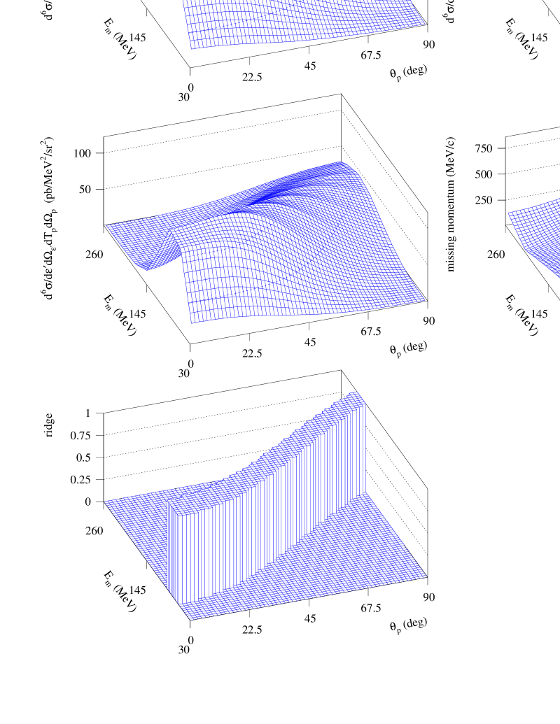
FIG. 2.: The calculated contribution from two-nucleon knockout to the differential ¹⁶O$(e,e^{\prime}p)$ cross section versus missing energy and proton angle at is $\epsilon$=1.2 GeV, $\epsilon^{\prime}$=0.9  GeV and $\theta_{e}$=16^o (or, $x\approx 0.15$ and $q=0.42$ GeV/c). The upper left panel includes solely the central correlations and the upper right panel has both central and tensor correlations. The lower left panel, on the other hand, includes apart from the central and tensor correlations also the MEC and IC. The variation of the missing momentum versus missing energy and proton angle is shown in the lower right panel. The lower left panel shows the position of the “ridge” in the $(E_{m},p_{m})$ plane. Hereby, the variable $<E_{x}^{hh^{\prime}}>$ was varied between 0. and 40. MeV.

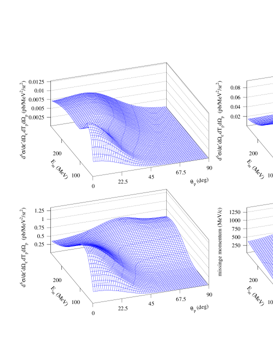
FIG. 3.: The calculated contribution from two-nucleon knockout to the differential ¹⁶O$(e,e^{\prime}p)$ cross section versus missing energy and proton angle at $\epsilon$=2.442 GeV, $\epsilon^{\prime}$=1.997  GeV and $\theta_{e}$=23.4^o (or, $x\approx 1$ and $q=1.0$ GeV/c). The upper left panel includes solely the central correlations and the upper right panel has both central and tensor correlations. The lower left panel, on the other hand, includes apart from the central and tensor correlations also the MEC and IC. The variation of the missing momentum versus missing energy and proton angle is shown in the lower right panel.

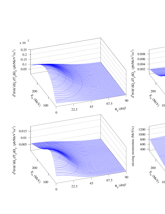
FIG. 4.: The calculated contribution from two-nucleon knockout to the differential ¹⁶O$(e,e^{\prime}p)$ cross section versus missing energy and proton angle at $\epsilon$=2.5 GeV, $\epsilon^{\prime}$=2.2  GeV and $\theta_{e}$=26.0^o (or, $x\approx 2$ and $q=1.1GeV/c$). The upper left panel includes solely the central correlations and the upper right panel has both central and tensor correlations. The lower left panel, on the other hand, includes apart from the central and tensor correlations also the MEC and IC. The variation of the missing momentum versus missing energy and proton angle is shown in the lower right panel.

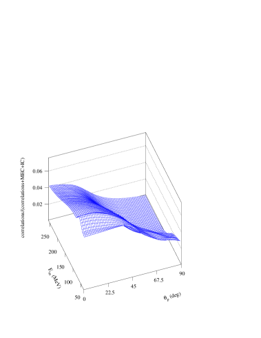
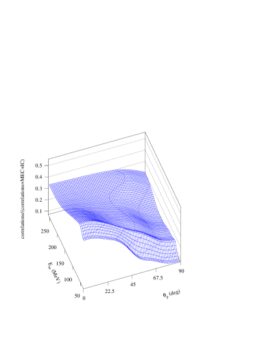
FIG. 5.: The ratio of the strength from the nucleon-nucleon correlations to the full semi-exclusive ¹⁶O$(e,e^{\prime}p)$ strength (including MEC and IC) versus proton angle and missing energy for the kinematical conditions considered in Figs. 3 (left panel) and 4 (right panel).

FIG. 6.: The longitudinal ($\sigma_{L}$) and transverse ($\sigma_{T}$) part of the differential ¹⁶O$(e,e^{\prime}p)$ cross section versus missing energy in parallel kinematics at $\epsilon$=1.2 GeV, $\epsilon^{\prime}$=0.9  GeV and $\theta_{e}$=16^o (or, $x\approx 0.15$ and $q=0.42$ GeV/c). The dashed line includes solely the central correlations ; the dot-dashed line both central and tensor correlations. The solid curves represent the calculations that include central and tensor correlations, as well as MEC and IC. Neither the MEC nor the IC do contribute to the longitudinal part of the cross section.

FIG. 7.: As in Figure 6 but for $\epsilon$=2.442 GeV, $\epsilon^{\prime}$=1.997  GeV and $\theta_{e}$=23.4^o (or, $x\approx 1$ and $q=1.0$ GeV/c).

FIG. 8.: As in Figure 6 but for $\epsilon$=2.5 GeV, $\epsilon^{\prime}$=2.2  GeV and $\theta_{e}$=26.0^o (or, $x\approx 2$ and $q=1.1$ GeV/c).

REFERENCES

• [1] L.J.H.M. Kester et al., Phys. Lett. B366 (1996) 44.
• [2] L.L. Frankfurt, M.M. Sargsian and M.I. Strikman, Phys. Rev. C 56 (1997) 1124.
• [3] I. Sick in Proceedings of the Workshop on Electron Nucleus Scattering, eds Omar Benhar and Adelchi Fabrocini (Edizioni ETS, Pisa, 1997) p. 445.
• [4] P. Demetriou, A. Gil, S. Boffi, C. Giusti, E. Oset and F.D. Pacati, Nucl. Phys. A650 (1999) 199.
• [5] A. Gil, J. Nieves and E. Oset, Nucl. Phys. A627 (1997) 599.
• [6] O. Benhar, S. Fantoni and G.I. Lykasov, Eur. Phys. J A 5 (1999) 137.
• [7] H. Morita, C. Ciofi degli Atti and D. Treleani, Phys. Rev. C 60 (1999) 034603.
• [8] Claudio Ciofi degli Atti and Daniele Treleani, Phys. Rev. C 60 (1999), 024602.
• [9] P.E. Ulmer et al., Phys. Rev. Lett. 59 (1987) 2259.
• [10] R.W. Lourie, W. Bertozzi, J. Morrison and L.B. Weinstein, Phys. Rev. C 57 (1993) R444.
• [11] N. Liyanage, Ph.D. thesis, MIT (1999).
• [12] M. Holtrop et al., Phys. Rev. C 58 (1998) 3205.
• [13] D. Dutta, Ph.D. thesis, Northwestern University (1999).
• [14] J. Ryckebusch, V. Van der Sluys, K. Heyde, H. Holvoet, W. Van Nespen, M. Waroquier and M. Vanderhaeghen, Nucl. Phys. A 624 (1997) 581.
• [15] J. Ryckebusch, M. Vanderhaeghen, L. Machenil and M. Waroquier, Nucl. Phys. A 568 (1994) 828-854.
• [16] S.C. Pieper, R.B. Wiringa and V.R. Pandharipande, Phys. Rev. C 46 (1992) 1741.
• [17] O. Benhar and V.R. Pandharipande, Rev. Modern Phys. 65 (1993) 817.
• [18] R. Guardiola, P.I. Moliner, J. Navarro, R.F. Bishop, A. Puente and Niels R. Walet, Nucl. Phys. A 609 (1996) 218.
• [19] V.R. Pandharipande and R.B. Wiringa, Rev. Mod. Phys. 51 (1979) 821.
• [20] S. Fantoni and V.R. Pandharipande, Nucl. Phys. A 473 (1987) 234.
• [21] H. Feldmeier, T. Neff, R. Roth and J. Schnack, Nucl. Phys. A 632 (1998) 61.
• [22] Gerald A. Miller and James E. Spencer, Annals of Physics 100 (1976) 562.
• [23] M. Vanderhaeghen, L. Machenil, J. Ryckebusch and M. Waroquier, Nucl. Phys. A 580 (1994) 551.
• [24] D. Abbott et al., Phys. Rev. Lett. 80 (1998) 5072.
• [25] C.C.Gearhart, PhD thesis, Washington University (St. Louis, 1994), unpublished and W. Dickhoff, private communication.
• [26] K.I. Blomqvist et al., Phys. Lett. B 421 (1998) 71.
• [27] Jan Ryckebusch, Dimitri Debruyne, Wim Van Nespen and Stijn Janssen, Phys. Rev. C 60 (1999) 034604.
• [28] C.J.G. Onderwater et al., Phys. Rev. Lett. 81 (1998) 2213.
• [29] R. Starink em et al., in press and Ph.D. Thesis, Free University of Amsterdam (1999), unpublished.
• [30] D. Van Neck, L. Van Daele, Y. Dewulf and M. Waroquier, Phys. Rev. C 56 (1997) 1398.
• [31] J.J. van Leeuwe et al., Nucl. Phys. A 631 (1998) 593c.
• [32] J.A. Templon, nucl-ex/9902008.
• [33] TJNAF experiment E97-106 “Studying the Internal Small-distance structure of Nuclei via the Triple Coincidence ($e,e^{\prime}p+N$) measurement” (spokesperson E. Piasetzky).
• [34] A. Bianconi, S. Jeschonnek, N.N. Nikolaev and B.G. Zakharov, Phys. Lett. B 363 (1995) 217.
Refer to caption