On the Response Function Technique for Calculating the Random-Phase Approximation Correlation Energy

Abstract

We develop a scheme to exactly evaluate the correlation energy in the random-phase approximation, based on linear response theory [1]. It is demonstrated that our formula is completely equivalent to a contour integral representation recently proposed in Ref. [4] being numerically more efficient for realistic calculations. Numerical examples are presented for pairing correlations in rapidly rotating nuclei.

Mean field theory provides a powerful approximation for describing many-particle systems. However, there are many situations where one is forced to go beyond mean field to include higher-order correlations, the random-phase approximation (RPA) being a widely used method for this purpose. One of the basic observables which require to go beyond mean field approximation is the correlation energy. In this case, the different RPA modes contribute in a democratic way. To calculate this quantity one has, therefore, to determine many RPA eigenmodes, especially in the case where symmetries of the mean-field are spontaneously broken, such as in the case of superfluid and deformed rotating nuclei. In Ref. [1] we developed a method to calculate the correlation energy in the RPA, making use of the response function techniques, and applied it to the study of pairing correlations in rapidly rotating nuclei. The essence of the method consists in expressing the RPA correlation as an integral in terms of the RPA response function, function which can be calculated without explicitly solving the RPA eigenvalue problem. These techniques have been recently extended to deal with the Nambu-Goldstone modes [2], and to calculate the nucleon effective mass in superfluid, deformed, and rotating nuclei [3].

Recently, a contour integral representation for the RPA correlation energy has been proposed in Ref. [4]. It was claimed that this method is more efficient than that developed in Ref. [1]. The assertion was also made that the method of Ref. [1] did not take the contribution of the spurious modes into account. In this letter we show that both methods are completely equivalent. Furthermore, using the property of meromorphic functions, we improve the original method of Ref. [1] to obtain the exact RPA correlation energy in more efficient way than that proposed in [4].

The Hamiltonian describing the system under discussion is

$$H=H_{0}+V,$$ (1)

where $H_{0}$ is the unperturbed one-body (mean-field) Hamiltonian and $V$ is the residual two-body interaction, which is assumed to be of the multi-separable form

$$V=-{1\over 2}\sum_{\rho}\chi_{\rho}Q_{\rho}Q_{\rho},$$ (2)

$Q_{\rho}$ being a one-body hermitian operator while $\chi_{\rho}$ is the strength of the interaction in channel $\rho$. The associated ground state energies and state vectors of $H_{0}$ and $H$ are denoted $E_{0}$, $|\Phi_{0}\rangle$ and $E$, $|\Psi\rangle$, respectively. Turning on the interaction adiabatically, the correlation energy can be written as [5]

$$E_{\rm corr}\equiv E-E_{0}=\int_{0}^{1}d\lambda\,\langle\Psi(\lambda)|V|\Psi(\lambda)\rangle.$$ (3)

In this equation $|\Psi(\lambda)\rangle$ is the ground state of the $\lambda$-scaled Hamiltonian $H(\lambda)\equiv H_{0}+\lambda V$. Within the RPA approximation, the correlation energy takes the form (see e.g. [6])

$$E_{\rm corr}^{\rm RPA}={1\over 2}\Bigl{[}\sum_{n}\omega_{n}-\sum_{\alpha<\beta}(E_{\alpha}+E_{\beta})\Bigr{]},$$ (4)

where $\omega_{n}$ is the RPA eigenfrequency and $E_{\alpha}+E_{\beta}$ is the unperturbed two-quasiparticle energy (eigenstates of $H_{0}$) in the quasiparticle representation. As shown in [1], the above expression can be rewritten as

$$E_{\rm corr}^{\rm RPA}=-{1\over 2\pi}\,\mathop{{\rm lim}}\limits_{\epsilon\rightarrow 0+}\,\int_{0}^{\infty}d\omega\,{\rm Im}\bigl{[}F(\omega+i\epsilon)\bigr{]},$$ (5)

where

$$F(\omega)\equiv\int_{0}^{1}d\lambda\,{\rm Tr}\Bigl{[}{\cal R}^{(\lambda)}(\omega)\chi\Bigr{]}.$$ (6)

The $\lambda$-scaled RPA response function (matrix) ${\cal R}^{(\lambda)}(\omega)$ is defined in term of the unperturbed response function (matrix),

$$R_{\rho\sigma}(\omega)\equiv\sum_{\alpha<\beta}\Bigl{[}{q_{\rho}^{*}(\alpha\beta)q_{\sigma}(\alpha\beta)\over E_{\alpha}+E_{\beta}-\omega}+{q_{\rho}(\alpha\beta)q_{\sigma}^{*}(\alpha\beta)\over E_{\alpha}+E_{\beta}+\omega}\Bigr{]},$$ (7)

as

$${\cal R}^{(\lambda)}(\omega)=\bigl{[}1-R(\omega)\chi\lambda\bigr{]}^{-1}R(\omega),$$ (8)

where $q_{\rho}(\alpha\beta)=\langle\alpha\beta|Q_{\rho}|0\rangle$ and $\chi=(\delta_{\rho\sigma}\chi_{\rho})$.

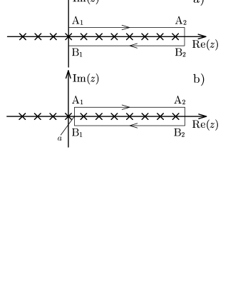
FIG. 1.: An illustration of the integration contour in the complex plane. Crosses denote the positions of the RPA and unperturbed roots, which give singularities of the funtcion $F(z)$, Eq. (9).

A small but finite value of the imaginary part $\epsilon\equiv{\rm Im}(\omega)$ has been used to evaluate the correlation energy in Ref. [1] (cf. Eq. 5) and found that it takes increasingly more computational time to approach the exact value of $E^{\rm RPA}_{\rm corr}$ ($\epsilon\rightarrow 0$). Here we show that Eqs. (5)$-$(8) are equivalent to the integral representation proposed in Ref. [4], and present a more efficient way to evalute the associated correlation energy than that presented in Ref. [4]. For this purpose, we make use of the analytic properties of the function $F(\omega)$, which become evident by carrying out the $\lambda$-integration in Eq. (6) analytically,

$$F(z)=-\log\bigl{(}\det\bigl{[}1-R(z)\chi\bigr{]}\bigr{)}.$$ (9)

Thus, $F(\omega)$ has logarithmic singularities at the RPA eigenenergies and at the two-quasiparticle unperturbed energies on the real axis. Eq. (5) can now be expressed as contour integral (see Fig. 1)

$$E_{\rm corr}^{\rm RPA}=-{1\over 4\pi i}\oint_{C_{\rm\ref{contr1}a}}dz\,F(z),$$ (10)

where $C_{\rm\ref{contr1}a}$ is a (closed) path which passes through the origin of the complex plane $z$, and which encloses all the positive RPA and unperturbed roots. Even if there is a spurious zero-energy mode (the symmetry-recovering mode or the Nambu-Goldstone mode) in the RPA spectrum, $F(\omega)\sim{\rm const.}\times\log z$ at $z\sim 0$ so that the integral converges at the origin. In order to show the equivalence of Eq. (10) to the corresponding formula of Ref. [4], we consider the integration path dipicted in Fig. 1b, where $a$ is a small positive quantity chosen to be smaller than the lowest singular point of $F(z)$. Integrating by parts, one obtain

$$\oint_{C_{\rm\ref{contr1}b}}dz\,F(z)=\bigl{[}zF(z)\bigr{]}_{C_{\rm\ref{contr1}b}}-\oint_{C_{\rm\ref{contr1}b}}dz\,z{d\over dz}F(z).$$ (11)

If the zero mode exists, the segment of the real axis between the origin and the lowest RPA (or two-quasiparitcle) root is a “branch-cut” of the complex logarithmic function $F(z)$, and so $\bigl{[}zF(z)\bigr{]}_{C_{\rm\ref{contr1}b}}=-2\pi ia$ (minus sign arizing from the fact that the direction of the path is clockwise). On the other hand, the singularities of the function $z{d\over dz}F(z)$ are poles at the same points as those of $F(z)$. Thus, in the limit $a\rightarrow 0$, the branch-cut contribution vanishes, and

$$E_{\rm corr}^{\rm RPA}={1\over 4\pi i}\oint_{C_{\rm\ref{contr1}b}}dz\,z{d\over dz}F(z),$$ (12)

which is nothing else than the integral representation of $E_{\rm corr}^{\rm RPA}$ of Ref. [4] (cf. Eq. (6) in it). Note that if there is a zero mode, ${d\over dz}F(z)\sim 1/z^{2}$, so the integral in Eq. (12) diverges when the path goes through the origin. Otherwise, the origin is not a singular point and the path $C_{\rm\ref{contr1}b}$ can be trivially modified into $C_{\rm\ref{contr1}a}$ in Eq. (12). If one uses the path $C_{\rm\ref{contr1}b}$ in Eq. (10) instead of $C_{\rm\ref{contr1}a}$, one has to add the branch-cut contribution $-a/2$ if the zero mode exists.

In spite of the equivalence mentioned above, Eq. (10) is numerically easier to calculate than Eq. (12) (or equivalently Eq. (6) of Ref. [4]), since the meromorphic function $F(z)$ has a more regular asymptotic behavior than $z{d\over dz}F(z)$. In fact, in the limit $|z|\rightarrow\infty$, $F(z)\rightarrow o(1/z^{2})$ while $z{d\over dz}F(z)\rightarrow o(1)$. Consequently, the contribution to the corresponding integral arising from the segment A₂B₂ in Fig. 1 vanishes when the points A₂ and B₂ are taken to infinity. Now the meaning of the approximation used in Ref. [1], is clear; the calculation of Eq. (5) with finite $\epsilon\equiv{\rm Im}(\omega)$ is equivalent to the integration along the path shown in Fig. 1a), except the contribution from the segment A₁B₁ which vanishes only in the limit of $\epsilon\equiv{\rm Im}(\omega)\rightarrow 0$. We have checked this point numerically.

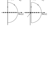
FIG. 2.: The modified integration contour from Fig. 1, which is more suitable to calculate the RPA correlation energy. One has to take the limit of infinite radius of the semicircle, whose contribution then vanishes.

For convenience, the integration path in Eq. (10) can be modified to the one shown in Fig. 2a). In this case the contribution from the semicircle vanishes as its radius goes to infinity. Moreover, the modification of the path parallel to the real axis into the one parallel to the imaginary axis is very useful for making the numerical calculations efficient. This is because ${\rm Im}F(z)$ is an oscillating function of ${\rm Re}(z)$ on the path shown in Fig. 1a), while ${\rm Re}F(z)$ is a rapidly decreasing function of Im(z) on the path shown in Fig. 2a). Consequently, one needs in this case a smaller set of mesh points to carry out the integration than in the case of the path shown in Fig. 1a). Therefore, the expression

$$E_{\rm corr}^{\rm RPA}=-{1\over 4\pi}\int_{-\infty}^{+\infty}d\omega\,{\rm Re}\bigl{[}F(i\omega)\bigr{]},$$ (13)

of the RPA correlation energy is numerically more convenient to evaluate than the expression displayed in Eq. (10) or (12), equivalent to Eq. (6) of Ref. [4]. It is worthwhile noticing that the integral appearing in Eq. (10) or (13), is further simplified by using the following properties of $F(z)$: $[F(z)]^{*}=F(-z^{*})$ and $F(-z)=F(z)$, which can be easily demonstrated making use of Eqs. (5) and (9). Consequently the integrand ${\rm Re}F(z)$ is symmetric with respect to the real axis, and $\int_{-\infty}^{+\infty}=2\int_{0}^{\infty}$ in Eq. (13). A similar simplification is possible in Eq. (10).

In Refs. [1, 7], the pairing correlations in rapidly rotating nuclei have been studied by using the general method discussed above. In these references, in addition to the RPA correlation energy, another measure of pairing correlations was introduced, namely the RPA pairing gap, ${\mit\Delta}_{{\rm RPA}}$ [7] (called the “effective” pairing gap in [1]). It is defined as

$${\mit\Delta}_{{\rm RPA}}\equiv\sqrt{{\mit\Delta}^{2}+{1\over 2}G^{2}\,S_{0}({{\rm RPA}})},$$ (14)

with

$$S_{0}({{\rm RPA}})\equiv\sum_{n\neq{\rm NG}}\Bigl{[}|\langle n|P|0\rangle|^{2}+|\langle n|P^{\dagger}|0\rangle|^{2}\Bigr{]}_{{\rm RPA}},$$ (15)

where ${\mit\Delta}=G\,\langle 0|P^{\dagger}|0\rangle_{\rm HB}$ is the standard, static BCS pairing gap (the order parameter of mean-field), while $G$ is the pairing force strength. The non-energy weighted sum rule $S_{0}({{\rm RPA}})$ describes the contribution of the RPA fluctuations for the monopole pair transfer operator, $P^{\dagger}=\sum_{i>0}c_{i}^{\dagger}c_{\tilde{i}}^{\dagger}$. Note that $\sum_{n\neq{\rm NG}}$ means that the divergent contribution from the spurious mode (pairing rotation) is to be excluded, in keeping with the fact that its contribution to Eq. 14 is included through the static pairing gap ${\mit\Delta}$. In Ref. [1], $S_{0}({{\rm RPA}})$ was calculated making use of the expression

$$S_{0}({{\rm RPA}})\approx{1\over\pi}\int_{\omega_{\rm cut}}^{\infty}d\omega\,{\rm Im}\,{\rm Tr}\bigl{[}{\cal R}(\omega+i\epsilon)\bigr{]},$$ (16)

where ${\cal R}(\omega)\equiv{\cal R}^{(\lambda=1)}(\omega)$ is the RPA response function, whose dimension is 2 corresponding to $Q_{1}=(P^{\dagger}+P)/\sqrt{2}$ and $Q_{2}=i(P^{\dagger}-P)/\sqrt{2}$. A finite value of $\epsilon$ and a low-energy cutoff $\omega_{\rm cut}$ are used to get rid of the NG mode contribution numerically. This is the same approximation as that used in calculating the RPA correlation energy [1], and can then be avoided in keeping with the discussion leading to Eqs. (10) and (13). In this case, the path in Fig. 2b) is to be used in order to avoid the singularity associated with an eventual zero mode, as in this case ${\cal R}(z)$ has a second order pole at the origin (cf. [2]):

$$S_{0}({{\rm RPA}})={1\over 2\pi}\int_{-\infty}^{+\infty}d\omega\,{\rm Re}\,{\rm Tr}\bigl{[}{\cal R}(a+i\omega)\bigr{]}.$$ (17)

Since the function ${\rm Tr}\bigl{[}{\cal R}(z)\bigr{]}$ has poles as singularities, the integral is independent of the choice of $a$. Summing up, making use of Eqs. (13) and (17), both the RPA correlation energy and the RPA pairing gap can be exactly evaluated in a numerically efficient way.

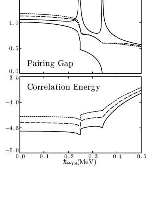
FIG. 3.: RPA Pairing gap (upper panel) and RPA correlation energy (lower panel) for neutrons in ¹⁶⁴Er as a function of the rotational frequency. Both quantities are in MeV. The solid, dashed and dotted lines denote the results of calculations with $\epsilon\equiv$ Im($\omega$) = 0 (exact), 100 keV and 200 keV, respectively. $\hbar\omega_{\rm cut}$ = 400 keV is used for the approximate (finite $\epsilon$) calculations of the RPA paring gap. The value of the static (mean-field) pairing gap $\Delta$, which vanishes at $\hbar\omega_{\rm rot}=0.34$ MeV, is also displayed in the upper panel.

In what follows we compare the results of the exact and approximate calculations of both $E^{\rm RPA}_{\rm corr}$ and ${\mit\Delta}_{\rm RPA}$ in the case of deformed, superfluid nuclei as a function of the rotational frequency (cf. Fig.(3)). Eqs. (13) and (17) were used to carry out the exact calculation, while Eqs. (5) and (16) with finite values of $\epsilon\equiv{\rm Im}(\omega)$ = 100, 200 keV were used to obtain the approximate results, as was been done in Refs. [1, 7] (${\rm Im}(\omega)$ = 80 keV was used in [1, 7]). The nucleus ¹⁶⁴Er has been chosen as a typical rotating nucleus and constant deformation parameters were used for simplicity. Only the monopole pairing force has been included with the smoothed pairing gap method being employed, which leads to a slightly different model space from that used in [1, 7]. Note that the correlation energy given in Eq. (4) as well as the sum rule value of the pairing gap given in Eq. (15) include the exchange (Fock) contribution. In Fig. 3, this contribution is excluded for the RPA pairing gap in accordance with Ref. [7], while it is included for the RPA correlation energy as in Ref. [1]. The cusp behaviours are clearly visible in the correlation energy, which are caused by the sudden change of the mean-field (static pairing gap); they are associated with the pairing phase-transition at $\hbar\omega_{{\rm rot}}=0.34$ MeV, and with the crossing of the $g$- and $s$-bands at $\hbar\omega_{{\rm rot}}=0.25$ MeV. They are more evident in the RPA pairing gap, where the “exact” ($\epsilon=0$) calculation diverges at these transition points. These divergences are due to a contribution of the lowest solution, which approaches to zero-energy at the transition points and brings about similar effects as those caused by the spurious mode, e.g. infinite strength. This is the well-known drawback of the RPA, whose small amplitude approximation breaks down near the transition points. The approximate results ($\epsilon\neq 0$) are very similar to the exact one ($\epsilon=0$) and provide accurate estimates of the rotational frequency dependence of both the correlation energy and the pairing gap, except at the transition points. In particular in the case of the pairing gap, the singular behaviour at these points are smooth out because of the low-energy cutoff $\hbar\omega_{\rm cut}$.

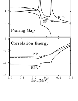
FIG. 4.: Comparison of the RPA and the number projection (NP) calculations of the pairing gap (upper panel) and correlation energy (lower panel) for neutrons in ¹⁶⁴Er as a function of the rotational frequency. The solid (dotted) lines denote the results of the RPA (NP) calculations. The results of approximate $\epsilon=200$ keV calculation in Fig. 3 are also included as dashed lines.

There is an another method which allows to go beyond mean-field approximation, namely number-projection (NP) (see e.g. [6]). The results of both methods were compared in Ref. [7], where the RPA calculation was carried out approximately as in [1]. Here we compare the NP results with the exact RPA results in Fig. 4. The NP correlation energy is defined as the energy difference between the NP and mean-field (Hartree-Bogoliubov), $E^{({\rm NP})}_{\rm corr}\equiv E_{\rm NP}-E_{\rm HB}$ (the exchange energy is included in $E_{\rm NP}$). Although RPA leads to larger values of the correlations, especially in the superfluid phase, the rotational frequency dependences are quite similar as already found in [7]. The advantage of the NP method over the RPA is to lead to smooth functions for both the correlation energy and the pairing gap at the pairing phase-transition point. It is, however, noticed that the cusp behaviour remains in the correlation energy at the $g$-$s$ crossing point.

In conclusion, a method to exactly deal with RPA correlations, based on that proposed in Ref. [1], has been developed. It is equivalent to a recently proposed integral representation in [4], and allows one to calculate the exact RPA correlation energy and in a numerically efficient way, properly dealing with the contribution of the Nambu-Goldstone modes. Making use of this method the pairing correlation in rapidly rotating nuclei can be studied in detail, providing the basis for an eventual analysis of the pairing phase-transition in strongly rotating nuclei.

This work is support in part by the Grant-in-Aid for Scientific Research from the Japan Ministry of Education, Science and Culture (No. 10640275).

REFERENCES

- [1] Y. R. Shimizu, J. D. Garrett, R. A. Broglia, M. Gallardo and E. Vigezzi, Rev. Mod. Phys. 61, 131 (1989).
- [2] P. Donati, T. Døssing, Y. R. Shimizu, P. F. Bortignon and R. A. Broglia, Nucl. Phys. A653, 27 (1999).
- [3] P. Donati, T. Døssing, Y. R. Shimizu, P. F. Bortignon and R. A. Broglia, Nucl. Phys. A653, 225 (1999).
- [4] F. Dönau, D. Almehed and R. G. Nazmitdinov, Phys. Rev. Lett. 83, 280 (1999).
- [5] A. L. Fetter and J. D. Walecka, Quantum Theory of Many-Particle Systems, (McGraw-Hill, New York, 1971).
- [6] P. Ring and P. Schuck, The Nuclear Many-Body Problem, (Springer-Verlag, New York, 1980).
- [7] Y. R. Shimizu and R. A. Broglia, Nucl. Phys. A515, 28 (1990);