coifeyn curly_len2mm dash_len1.5mm wiggly_len3mm

vardef ellipseraw (expr p, ang) = save radx; numeric radx; radx=6/10 length p; save rady; numeric rady; rady=3/10 length p; pair center; center:=point 1/2 length(p) of p; save t; transform t; t:=identity xscaled (2*radx*h) yscaled (2*rady*h) rotated (ang + angle direction length(p)/2 of p) shifted center; fullcircle transformed t enddef; style_def ellipse expr p= shadedraw ellipseraw (p,0); enddef;

A Sketch of Two and Three Bodies

Abstract

A cartoon of the Effective Field Theory of many nucleon systems is drawn, concentrating on Compton scattering in the two nucleon system, and on $nd$ scattering in the three body system.

The purpose of this presentation is to give a concise introduction into the Effective Field Theory (EFT, for a review see e.g. LepageQEDlecture ) of two and three nucleon systems as it emerged in the last three years. However, I can only give a “teaser” with a lot of words and figures and a few cheats in details, referring to the literature, esp. to the excellent proceedings of the INT-Caltech Workshops 1998 and 1999 INTWorkshopSummary . I concentrate on work undertaken with J.-W. Chen, R.P. Springer and M.J. Savage in pola ; Compton , P.F. Bedaque in pbhg ; pbfghg , and F. Gabbiani in pbfghg . M. Birse’s talk at this Workshop provides a more formal investigation of the EFT of the two nucleon system, and U.-G. Meißner’s alternative approach he presented here follows Weinberg’s original suggestion Weinberg but needs to be studied further.

Effective Field Theory methods are largely used in many branches of physics where a separation of scales exists. In low energy nuclear systems, the two well separated scales are, on one side, the low scales of the typical momentum of the process considered and the pion mass, and on the other side the higher scales associated with chiral symmetry and confinement. This separation of scales was explored with great success in the mesonic sector (Chiral Perturbation Theory leutWeinberg79 ) and in the one baryon sector (Heavy Baryon Chiral Perturbation Theory GasseretalJenkinsManohar ), producing a low energy expansion of a variety of observables (see also the Chiral Perturbation Theory section of this Workshop). It provided for the first time a description of strongly interacting particles which is systematic, rigorous and model independent (meaning, independent of assumptions about the non-perturbative QCD dynamics).

Three main ingredients enter the construction of an EFT: The Lagrangean, the power counting and a regularisation scheme. First, the relevant degrees of freedom have to be identified. In his original suggestion how to extend EFT methods to systems containing two or more nucleons, Weinberg Weinberg noticed that below the $\Delta$ production scale, only nucleons and pions need to be retained as the infrared relevant degrees of freedom of low energy QCD. Because at these scales the momenta of the nucleons are small compared to their rest mass, the theory becomes non-relativistic at leading order in the velocity expansion, with relativistic corrections systematically included at higher orders. The most general chirally (and iso-spin) invariant Lagrangean consists hence of contact interactions between non-relativistic nucleons, and between nucleons and pions, with the first few terms of the form

$${\mathcal{L}}_{NN} = N^{\dagger}({\rm i}\partial_{0}+\frac{\vec{\partial}^{2}}{2M})N+\;\frac{f_{\pi}^{2}}{8}\;{\rm tr}[(\partial_{\mu}\Sigma^{\dagger})(\partial^{\mu}\Sigma)]\;+\;g_{A}N^{\dagger}\vec{A}\cdot\sigma N\;-$$

$$-\;C_{0}(N^{{\rm T}}P^{i}N)^{\dagger}\ (N^{{\rm T}}P^{i}N)\;+$$

$$+\;\frac{C_{2}}{8}\left[(N^{{\rm T}}P^{i}N)^{\dagger}(N^{{\rm T}}P^{i}(\stackrel{{\scriptstyle\scriptscriptstyle\rightarrow}}{{\partial}}-\stackrel{{\scriptstyle\scriptscriptstyle\leftarrow}}{{\partial}})^{2}N)+{\rm h.c.}\right]+\dots\;\;,$$

where $N={p\choose n}$ is the nucleon doublet of two-component spinors and $P^{i}$ is the projector onto the iso-scalar-vector channel, $P^{i,\,b\beta}_{a\alpha}=\frac{1}{\sqrt{8}}(\sigma_{2}\sigma^{i})_{\alpha}^{\beta}(\tau_{2})_{a}^{b}$. $\sigma$ ($\tau$) are the Pauli matrices acting in spin (iso-spin) space. The iso-vector-scalar part of the $NN$ Lagrangean introduces more constants $C_{i}$ and interactions and has not been displayed for convenience. The field $\xi$ describes the pion, $\xi(x)=\sqrt{\Sigma}=e^{{\rm i}\Pi/f_{\pi}}$, $f_{\pi}=130\;{\rm MeV}$. $D_{\mu}$ is the chiral covariant derivative $D_{\mu}=\partial_{\mu}+V_{\mu}$, and the vector and axial currents are $V_{\mu}=\frac{1}{2}(\xi\partial_{\mu}\xi^{\dagger}+\xi^{\dagger}\partial_{\mu}\xi)$, $A_{\mu}=\frac{{\rm i}}{2}(\xi\partial_{\mu}\xi^{\dagger}-\xi^{\dagger}\partial_{\mu}\xi)$. The interactions involving pions are severely restricted by chiral invariance. As such, the theory is an extension to the many nucleon system of Chiral Perturbation Theory and Heavy Baryon Chiral Perturbation Theory. Like in its cousins, all short distance physics – branes and strings, quarks and gluons, resonances like the $\Delta$ or $\sigma$ – is integrated out into the coefficients of the low energy Lagrangean. In principle, these constants could be derived by solving QCD or via models of the short distance physics like resonance saturation. The most common and practical way to determine those constants, though, is by fitting them to experiment.

The EFT with pions integrated out (formally, $g_{A}=0$ in (A Sketch of Two and Three Bodies)) is valid below the pion cut and was recently pushed to very high orders in the two-nucleon sector CRS where accuracies of the order of $1\%$ were obtained. It can be viewed as a systematisation of Effective Range Theory with the inclusion of relativistic and short distance effects traditionally left out in that approach.

Because the Lagrangean (A Sketch of Two and Three Bodies) consists of infinitely many terms only restricted by symmetry, an EFT may at first sight suffer from lack of predictive power. Indeed, as the second part of its formulation, predictive power is ensured only by establishing a power counting scheme, i.e. a way to determine at which order in a momentum expansion different contributions will appear, and keeping only and all the terms up to a given order. The dimensionless, small parameter on which the expansion is based is the typical momentum $Q$ of the process in units of the scale $\Lambda$ at which the theory is expected to break down, with estimates ranging from $\Lambda_{\pi}\approx 300$ to $800\;{\rm MeV}$ INTWorkshopSummary in the two body system for the theory with pions. The pion-less theory should be in disagreement with experiment starting at the pion cut, $\Lambda_{{\rm no\pi}}\approx 140\;{\rm MeV}$. Values for $\Lambda$ and $Q$ have to be determined from comparison to experiments and are a priori unknown. Assuming that all contributions are of natural size, i.e. ordered by powers of $Q$, the systematic power counting ensures that the sum of all terms left out when calculating to a certain order in $Q$ is smaller than the last order retained, allowing for an error estimate of the final result.

Even if calculations of nuclear properties were possible starting from the underlying QCD Lagrangean, EFT simplifies the problem considerably by factorising it into a short distance part (subsumed into the coefficient of the Lagrangean) and a long distance part which contains the infrared-relevant physics and is dealt with by EFT methods. EFT provides an answer of finite accuracy because higher order corrections are systematically calculable and suppressed in powers of $Q$. Hence, the power counting allows for an error estimate of the final result, with the natural size of all neglected terms known to be of higher order. Relativistic effects, chiral dynamics and external currents are included systematically, and extensions to include e.g. parity violating effects are straightforward. Gauged interactions and exchange currents are unambiguous. Results obtained with EFT are easily dissected for the relative importance of the various terms. Because only $S$-matrix elements between on-shell states are observables, ambiguities nesting in “off-shell effects” are absent. On the other hand, because only symmetry considerations enter the construction of the Lagrangean, EFTs are less restrictive as no assumption about the underlying QCD dynamics is incorporated.

In systems involving two or more nucleons, establishing such a power counting is complicated by the fact that unnaturally large scales have to be accommodated, so that some coefficients in the Lagrangean may not be of natural size and hence possibly jeopardise power counting: Given that the typical low energy scale in the problem should be the mass of the pion as the lightest particle emerging from QCD, fine tuning seems to be required to produce the large scattering lengths in the ${}^{1}{\rm S}_{0}$ and ${}^{3}{\rm S}_{1}$ channels ($1/a^{{}^{1}{\rm S}_{0}}=-8.3\;{\rm MeV},\;1/a^{{}^{3}{\rm S}_{1}}=36\;{\rm MeV}$). Since there is a bound state in the ${}^{3}{\rm S}_{1}$ channel with a binding energy $B=2.225\;{\rm MeV}$ and hence a typical binding momentum $\gamma=\sqrt{MB}\simeq 46\;{\rm MeV}$ well below the scale $\Lambda$ at which the theory should break down, it is also clear that at least some processes have to be treated non-perturbatively in order to accommodate the deuteron. Most likely, these small scales do not arise from the fact that the real world is close to the chiral limit: In the singlet channel, for instance, the one pion exchange potential vanishes in the chiral limit and thus cannot be the cause of the fine tuning. The fine tuning then must be a result of short distance physics.

A way to incorporate this fine tuning into the power counting was suggested by Kaplan, Savage and Wise KSW : At very low momenta, contact interactions with several derivatives – like $p^{2}C_{2}$ and the pion-nucleon interactions – should become unimportant, and we are left only with the contact interactions proportional to $C_{0}$. The leading order contribution to nucleons scattering in an ${\rm S}$ wave comes hence from four nucleon contact interactions and is summed geometrically as in Fig. 1 to all orders to produce the shallow real bound state, i.e. the deuteron.

$\mbox{\parbox{25.0pt}{ \fmfgraph*(25,25) \fmfleft{i} \fmfright{o} \fmf{double,width=thin}{i,o} }}\hskip 5.0pt=\hskip 5.0pt\mbox{\parbox{30.0pt}{ \fmfgraph*(30,25) \fmfleft{i1,i2} \fmfright{o1,o2} \fmf{vanilla,width=thin}{i1,v,o2} \fmf{vanilla,width=thin}{i2,v,o1} }}\hskip 5.0pt+\hskip 5.0pt\mbox{\parbox{45.0pt}{ \fmfgraph*(45,25) \fmfleft{i1,i2} \fmfright{o1,o2} \fmf{vanilla,width=thin,tension=6}{i1,v1} \fmf{vanilla,width=thin,tension=6}{v2,o2} \fmf{vanilla,width=thin,tension=6}{i2,v1} \fmf{vanilla,width=thin,tension=6}{v2,o1} \fmf{vanilla,width=thin,left=0.5}{v1,v2} \fmf{vanilla,width=thin,left=0.5}{v2,v1} }}\hskip 5.0pt+\hskip 5.0pt\mbox{\parbox{63.0pt}{ \fmfgraph*(63,25) \fmfleft{i1,i2} \fmfright{o1,o2} \fmf{vanilla,width=thin,tension=6}{i1,v1} \fmf{vanilla,width=thin,tension=6}{v2,o2} \fmf{vanilla,width=thin,tension=6}{i2,v1} \fmf{vanilla,width=thin,tension=6}{v2,o1} \fmf{vanilla,width=thin,left=0.7}{v1,v3} \fmf{vanilla,width=thin,left=0.7}{v3,v1} \fmf{vanilla,width=thin,left=0.7}{v2,v3} \fmf{vanilla,width=thin,left=0.7}{v3,v2} }}+\;\dots\;=\;\displaystyle\frac{-C_{0}}{1-\rule{0.0pt}{12.0pt}\mbox{\parbox{24.0pt}{ \fmfgraph*(25,12) \fmfleft{i} \fmfright{o} \fmf{vanilla,width=thin,left=0.5}{i,o} \fmf{vanilla,width=thin,left=0.5}{o,i} }}}$

Figure 1: Re-summation of the contact interactions into the deuteron propagator.

How to justify this? Any diagram can be estimated by scaling momenta by a factor of $Q$ and non-relativistic kinetic energies by a factor of $Q^{2}/M$. The remaining integral includes no dimensions and is taken to be of the order $Q^{0}$ and of natural size. This scaling implies the rule that nucleon propagators contribute one power of $M/Q^{2}$ and each loop a power of $Q^{5}/M$. Assuming that

$$C_{0}\sim\frac{1}{MQ} \;\;,\;\; C_{2}\sim\frac{1}{M\Lambda Q^{2}}\;\;,$$ (2)

the diagrams contributing at leading order to the deuteron propagator are indeed an infinite number as shown in Fig. 1, each one of the order $1/(MQ)$. The regulator dependent, linear divergence in each of the bubble diagrams does not show in dimensional regularisation as a pole in $4$ dimensions, but it does appear as a pole in $3$ dimensions which we subtract following the Power Divergence Subtraction scheme KSW . Dimensional regularisation is chosen to explicitly preserve the systematic power counting as well as all symmetries (esp. chiral invariance) at each order in every step of the calculation. At leading (LO), next-to-leading order (NLO) and often even NNLO in the two nucleon system, it also allows for simple, closed answers whose analytic structure is readily asserted. The deuteron propagator

$$\frac{4\pi}{M}\;\frac{-{\rm i}}{\frac{4\pi}{MC_{0}}+\mu-\sqrt{\frac{\vec{\,\!p}\!\>{}^{2}}{4}-Mp_{0}-{\rm i}\varepsilon}}$$ (3)

has the correct pole position and cut structure when one chooses

$$C_{0}(\mu)=\frac{4\pi}{M}\;\frac{1}{\gamma-\mu}\;\;.$$ (4)

Indeed, when choosing $\mu\sim Q$, the leading order contact interaction scales as demanded in (2) and – as expected for a physical observable – the $NN$ scattering amplitude becomes independent of $\mu$, the renormalisation scale or cut-off chosen. The same can be shown for the higher order coefficients, so that the scheme is self-consistent. Power Divergence Subtraction moves hence a somewhat arbitrary amount of the short distance contributions from loops to counterterms and makes precise cancellations manifest which arise from fine tuning. Notice that the re-summed deuteron propagator has the same order $1/(MQ)$ as each diagram in Fig. 1.

One surprising result arises from this analysis because chiral symmetry implies a derivative coupling of the pion to the nucleon at leading order. The contribution from one pion exchange includes a factor of $Q^{-2}$ from the pion propagator and a factor of $Q^{2}$ coming from the pion-nucleon vertices, so that for momenta of the order of the pion mass, the instantaneous one pion exchange scales as $Q^{0}$ and is smaller than the contact piece $C_{0}$ which according to (2) scales as $Q^{-1}$. Iterated and radiative pion exchanges are suppressed even further. Pion exchange and higher derivative contact terms appear hence only as perturbations at higher orders. In contradistinction to iterative potential model approaches, each higher order contribution is inserted only once. In this scheme, the only non-perturbative physics responsible for nuclear binding is extremely simple, and the more complicated pion contributions are at each order given by a finite number of diagrams. For example, the NLO contributions to the deuteron are the one instantaneous pion exchange and the four nucleon interaction with two derivatives, Fig. 2. The constants are determined e.g. by demanding the correct deuteron pole position and residue PRS .

(60,30) i o double,width=thin,tension=8i,v1 double,width=thin,tension=8v2,o vanilla,width=thin,left=0.65v1,v2 vanilla,width=thin,left=0.65v2,v1 pa pavpath(__v1,__v2) pb pbvpath(__v2,__v1) dashespoint 1/2 length(pa) of pa – point 1/2 length(pb) of pb   +   (90,40) i o double,width=thin,tension=5i,v1 double,width=thin,tension=5v2,o vanilla,width=thin,left=0.8v1,v3 vanilla,width=thin,left=0.8v3,v1 vanilla,width=thin,left=0.8v2,v3 vanilla,width=thin,left=0.8v3,v2 decor.shape=square,decor.size=5,label=$\scriptstyle p^{2}C_{2}$, label.angle=90,label.dist=0.18wv3

Figure 2: The NLO corrections to the deuteron.

In the two body sector, the theory thus emerging has been put to extensive tests at NLO and NNLO, giving for the first time analytic answers to many deuteron properties, see e.g. INTWorkshopSummary . Although in general process dependent, the expansion parameter is found to be of the order of $\frac{1}{3}$ in most applications, so that NLO calculations can be expected to be accurate to about $10\%$, and NNLO calculations to about $4\%$. In all cases, experimental agreement is within the estimated theoretical uncertainties, and in some cases, previously unknown counterterms could be determined.

The elastic deuteron Compton scattering diagrams to NLO are partially obtained by gauging the Lagrangean (A Sketch of Two and Three Bodies), i.e. by replacing ordinary derivatives by covariant ones: At LO, a seagull-graph and one graph in which the incident and outgoing photon couple to the same nucleon are found. At NLO, the photons are attached in all possible ways to the corrections in Fig. 2, including to the pion, the $NN\pi$ vertex and the $C_{2}$ vertex. The Fermi interaction $\vec{\sigma}\cdot\vec{B}$ probes the ${}^{1}{\rm S}_{0}$ intermediate $NN$ state and enters at NLO, too. Finally, the iso-scalar electric nuclear polarisability was shown to come from relativistic (“radiative”) pions in Chiral Perturbation Theory BKMa , $\alpha_{E,N}=\frac{5g_{A}^{2}\alpha}{48\pi{f_{\pi}^{2}}m_{\pi}}$, and is NLO. The cross section fits finally on less than one page with functions not more complicated than Logarithms and Arcustangentes Compton and contains no free parameters. Comparison with the Urbana experiment Lucas in Fig. 3 shows good agreement, with the pion graphs that dominate the electric polarisability of the nucleon necessary to improve it. The deuteron scalar and tensor electric and magnetic polarisabilities are also easily extracted pola .

       

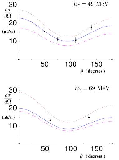
Figure 3: The differential cross section for elastic $\gamma$-deuteron Compton scattering at incident photon energies of $E_{\gamma}=49\ {\rm MeV}$ and $69\ {\rm MeV}$ in an EFT with explicit pions Compton , no free parameters. Dashed: LO; dotted: NLO without the graphs that contribute to the nucleon polarisability; solid curve: complete NLO result.

In the three body sector, even the leading order calculation is too complex for a fully analytical solution. Still, the equations that need to be solved are computationally trivial and can furthermore be improved systematically by higher order corrections that involve only (partly analytical, partly numerical) integrations, as opposed to many-dimensional integral equations arising in other approaches. The $nd$ system provides a laboratory in which many complications of the other channels are not encountered: The absence of Coulomb interactions ensures that only properties of the strong interactions are probed. In the quartet channel, the Pauli principle forbids three body forces Stooges in the first few orders. Because the calculation is parameter-free, it allows one to determine the range of validity of the KSW scheme without a detailed analysis of the fitting procedure. Although e.g. the quartet scattering length is large, no extra fine tuning except the one for the deuteron is required. In the ${\rm S}$ wave, spin-doublet (triton) channel, the situation is more complicated. An unusual renormalisation of the three-body force makes it large and as important as the leading two-body forces Stooges2 . More work is needed there.

A comparative study between the theory with explicit pions and the one with pions integrated out was performed in pbhg for the spin quartet ${\rm S}$ wave. As seen above, the two theories are identical at LO: All graphs involving only $C_{0}$ interactions are of the same order and form a double series which is not geometrical and cannot be summed analytically. One is hence left with the task of summing all “pinball” diagrams (first line of Fig. 4). Summing all “bubble-chain” sub-graphs into the deuteron propagator, one can however obtain the solution numerically from the integral equation pictorially shown in the lower line of Fig 4. A code runs within seconds on a personal computer.

(50,50) i2,i1 o2,o1 double,tension=6i1,v1,v2 vanilla,width=thinv2,o1 double,tension=6v3,v4,o2 vanilla,width=thini2,v3 vanilla,width=thinv2,v3 $+$ (80,50) i2,i1 o2,o1 double,tension=4i1,v1 vanilla,width=thinv1,v2 double,tension=4o1,v2 vanilla,width=thini2,v3 vanilla,width=thinv3,o2 vanilla,width=thinv2,v3 vanilla,width=thinv3,v1 $+$ (110,50) i2,i1 o2,o1 double,tension=8i1,v1 vanilla,width=thinv1,v2 double,tension=8o1,v2 double,tension=100v3,v3a double,tension=100v4,v4a phantomv3a,v4a vanilla,width=thini2,v3 vanilla,width=thinv4,o2 vanilla,width=thinv2,v4 vanilla,width=thinv3,v1 vanilla,width=thin,left=0.65v3a,v4a vanilla,width=thin,left=0.65v4a,v3a $+$ (110,50) i2,i1 o2,o1 double,tension=8i1,v1 vanilla,width=thinv1,v4 double,tension=100v4,v5 vanilla,width=thin,tension=1.666v5,o1 double,tension=8o2,v6 vanilla,width=thinv6,v3 double,tension=100v3,v2 vanilla,width=thin,tension=1.666v2,i2 vanilla,width=thinv1,v2 vanilla,width=thinv3,v4 vanilla,width=thinv5,v6 $+\;\dots$

(90,50) i2,i1 o2,o1 double,width=thin,tension=3i1,v1 double,width=thin,tension=1.5v1,v3,v2 double,width=thin,tension=3v2,o1 vanilla,width=thini2,v4,o2 ellipse,rubout=1v3,v4   $=$   (90,50) i2,i1 o2,o1 double,width=thin,tension=4i1,v1,v2 vanilla,width=thinv2,o1 double,width=thin,tension=4v3,v4,o2 vanilla,width=thini2,v3 vanilla,width=thinv2,v3   $+$   (170,50) i2,i1 o2,o1 double,width=thin,tension=3i1,v1 double,width=thin,tension=1.5v1,v6,v5 double,width=thin,tension=3v5,v2 vanilla,width=thinv2,o1 vanilla,width=thini2,v7 vanilla,width=thin,tension=0.666v7,v4 double,width=thin,tension=4v4,v3,o2 vanilla,width=thinv4,v2 ellipse,rubout=1v6,v7

Figure 4: The double infinite series of LO “pinball” diagrams, some of which are shown in the first line, is equivalent to the solution of the Faddeev equation shown in the second line.

The power counting shows that at NLO, we have additional contributions from: $p^{2}C_{2}$ insertions and pion exchange corrections to the deuteron propagator depicted in the first line of Fig. 5; pionic vertex corrections to $C_{0}$ (second line); and the pion diagram of the last line which corrects the three particle intermediate state. Here, we used a re-formulation of the Lagrangean (A Sketch of Two and Three Bodies) in order not to have poorly convergent diagrams containing $C_{2}$ like the second one in the first line of Fig. 4, see pbhg for details. The calculation without explicit pions was carried out to NNLO.

(200,50) i2,i1 o2,o1 double,width=thin,tension=3i1,v1 double,width=thin,tension=1.5v1,v3,v2 double,width=thin,tension=3v2,v5 decor.shape=square,decor.size=5,label=$\scriptstyle p^{2}C_{2}$,label.angle=90,label.dist=0.08wv5 double,width=thin,tension=3v5,v7 double,width=thin,tension=1.5v7,v8,v9 double,width=thin,tension=3v9,o1 vanilla,width=thini2,v4 vanilla,width=thin,tension=0.5v4,v10 vanilla,width=thinv10,o2 ellipse,rubout=1v3,v4 ellipse,rubout=1v8,v10 vanilla,width=thinv3,v4 vanilla,width=thinv8,v10 $+$ (200,50) i2,i1 o2,o1 double,width=thin,tension=3i1,v1 double,width=thin,tension=1.5v1,v3,v2 double,width=thin,tension=3v2,v5 vanilla,width=thin,left=0.8,tension=0.5v5,v6 vanilla,width=thin,left=0.8,tension=0.5v6,v5 double,width=thin,tension=3v6,v7 double,width=thin,tension=1.5v7,v8,v9 double,width=thin,tension=3v9,o1 vanilla,width=thini2,v4 vanilla,width=thin,tension=0.333v4,v10 vanilla,width=thinv10,o2 ellipse,rubout=1v3,v4 ellipse,rubout=1v8,v10 vanilla,width=thinv3,v4 vanilla,width=thinv8,v10 pa pavpath(__v5,__v6) pb pbvpath(__v6,__v5) dashespoint 1/2 length(pa) of pa – point 1/2 length(pb) of pb $+$

$+$ (100,50) i2,i1 o2,o1 double,width=thin,tension=2.5i1,v1 vanilla,width=thinv1,v3,o1 double,width=thin,tension=5o2,v2 vanilla,width=thinv2,i2 vanilla,width=thin,tension=1.7v2,v4 vanilla,width=thinv4,v1 dashes,width=thinv4,v3 $+\;2$ (150,50) i2,i1 o2,o1 double,width=thini1,i1a,v1 vanilla,width=thinv1,v3,o1 double,width=thin,tension=5o2,v2 vanilla,width=thinv2,i2a vanilla,width=thin,tension=2.5i2a,i2 vanilla,width=thin,tension=2v2,v4 vanilla,width=thinv4,v1 dashes,width=thinv4,v3 ellipse,rubout=1i1a,i2a vanillai1a,i2a $+$ (200,50) i2,i1 o2,o1 double,width=thini1,i1a,v1 vanilla,width=thinv1,v1a,v3 vanilla,width=thinv3,o1a,o1 double,width=thinv4,o2a,o2 vanilla,width=thin,tension=0.5v4,v2 vanilla,width=thinv2,i2a,i2 vanilla,width=thinv1,v5 vanilla,width=thinv5,v4 dashes,width=thinv5,v1a ellipse,rubout=1 i1a,i2a vanillai1a,i2a ellipse,rubout=1 o1a,o2a vanillao1a,o2a $+$

$+$ (100,50) i2,i1 o2,o1 double,width=thin,tension=3i1,v1 vanilla,width=thin,tension=1.6v1,v3 vanilla,width=thinv3,o1 double,width=thin,tension=3o2,v2 vanilla,width=thin,tension=1.6v2,v5 vanilla,width=thinv5,i2 vanilla,width=thinv2,v4 phantom,tension=3v4,v4a vanilla,width=thinv4a,v1 dashes,width=thinv3,v5 $+\;2$ (150,50) i2,i1 o2,o1 double,width=thin,tension=1.5i1,i1a,v1 vanilla,width=thin,tension=1.6v1,v3 vanilla,width=thinv3,o1 double,width=thin,tension=3o2,v2 vanilla,width=thin,tension=2.3v2,v5 vanilla,width=thinv5,i2a vanilla,width=thin,tension=1.9i2a,i2 dashes,width=thinv3,v5 ellipse,rubout=1 i1a,i2a vanillai1a,i2a vanilla,width=thin,tension=1.2v2,v4 phantom,tension=3v4,v4a vanilla,width=thinv4a,v1 $+$ (200,50) i2,i1 o2,o1 double,width=thini1,i1a,v1 vanilla,width=thinv1,v1a,v3 vanilla,width=thinv3,o1a,o1 double,width=thinv4,o2a,o2 vanilla,width=thinv4,v2a,v2 vanilla,width=thinv2,i2a,i2 vanilla,width=thinv1,v5a phantom,width=thin,tension=3v5b,v5a vanilla,width=thinv5b,v4 dashes,width=thinv2a,v1a ellipse,rubout=1 i1a,i2a vanillai1a,i2a ellipse,rubout=1 o1a,o2a vanillao1a,o2a

Figure 5: The NLO contributions to $nd$ scattering in the quartet channel. First line: Corrections to the deuteron propagator; second line: pionic corrections to the $C_{0}$ vertex ; third line: pionic corrections to three particle breakup in the intermediate state. Permuted graphs left out.

All calculations demonstrate convergence. The scattering length is $a({}^{4}S_{\frac{3}{2}},{\rm LO})=(5.1\pm 1.5)\;{\rm fm}$, and at NLO with (without) perturbative pions $a({}^{4}S_{\frac{3}{2}},{\rm NLO,\pi})=(6.8\pm 0.7)\;{\rm fm}$ ($a({}^{4}S_{\frac{3}{2}},{\rm NLO,{\rm no}\pi})=(6.7\pm 0.7)\;{\rm fm}$). At NNLO, Stooges report $a({}^{4}S_{\frac{3}{2}},{\rm NNLO,{\rm no}\pi})=(6.33\pm 0.1)\;{\rm fm}$, and the experimental value is $a({}^{4}S_{\frac{3}{2}},{\rm exp})=(6.35\pm 0.02)\;{\rm fm}$ Dilgetal . Comparing the NLO correction to the LO scattering length provides one with the familiar error estimate at NLO: $(\frac{1}{3})^{2}\approx 10\%$. The NLO calculations with and without pions lie within each other’s error bar. The NNLO calculation is inside the error ascertained to the NLO calculation and carries itself an error of about $(\frac{1}{3})^{3}\approx 4\%$. NLO and LO contributions become comparable for momenta of more than $200\;{\rm MeV}$. In the imaginary part shown in Fig. 6, the same pattern emerges with a slightly more pronounced difference between the pion-less and pions-full theory. Because results obtained with EFT are easily dissected for the relative importance of the various terms, one concludes that pionic corrections to $nd$ scattering in the quartet ${\rm S}$ wave channel – although formally NLO – are indeed much weaker: The calculation with perturbative pions and with pions integrated out do not differ significantly over a wide range of momenta. The difference should appear for momenta of the order of $m_{\pi}$ and higher because of non-analytical contributions of the pion cut. However, it is very moderate for momenta of up to $300\;{\rm MeV}$ in the centre-of-mass frame ($E_{{\rm cm}}\approx 70\;{\rm MeV}$), see Fig. 6. This and the lack of data makes it difficult to assess whether the KSW power counting scheme to include pions as perturbative increases the range of validity over the pion-less theory, but effects from the pion cut are seemingly weak.

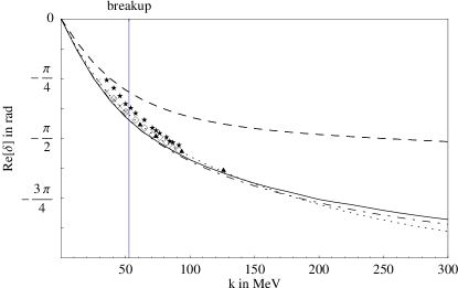
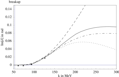
Figure 6: Real and imaginary parts in the quartet ${\rm S}$ wave phase shift of $nd$ scattering versus the centre-of-mass momentum pbhg . Dashed: LO; solid (dot-dashed) line: NLO with perturbative pions (pions integrated out); dotted: NNLO without pions Stooges ; pbfghg . Realistic potential models: squares from WitalaTUNL , crosses from Kievsky , triangles from Hueberetal . Stars: TUNL $pd$ phase shift analysis WitalaTUNL .

Finally, the real and imaginary parts of the higher partial waves $l=1,\dots,4$ in the spin quartet and doublet channel were presented in pbfghg in a papameter-free calculation. Figure 7 shows two examples. Comparison of the LO with the NLO and NNLO result demonstrates convergence of the EFT, with the expansion parameter again about $\frac{1}{3}$. It is interesting that the NLO correction is for high enough energies sometimes sizeable, while the NNLO correction is in general very small.

       

       

Figure 7: Real and imaginary parts of the quartet ${\rm P}$ (top) and doublet ${\rm F}$ (bottom) wave phase shift of $nd$ scattering versus the centre-of-mass energy in the EFT without pions pbfghg . Dashed: LO; dot-dashed: NLO; solid line: NNLO. The experiments by Huttel et al. Hutteletal and Schmelzbach et al. Schmelzbachetal are denoted by open squares and diamonds, respectively. The calculations of Kievsky et al. (crosses) are from Refs. Kievsky below breakup ($E_{{\rm cm}}=B$) and Kievskyprivcomm above breakup.

Within the range of validity of this pion-less theory, convergence is good, and the results agree with potential model calculations (as available) within the theoretical uncertainty. That makes one optimistic about carrying out higher order calculations of problematic spin observables like the $A_{y}$ problem where the EFT approach will differ from potential model calculations due to the inclusion of three-body forces.

Acknowledgements

It is a great pleasure to thank my collaborators – J.-W. Chen, R.P. Springer and M.J. Savage in pola ; Compton , P.F. Bedaque in pbhg ; pbfghg , and F. Gabbiani in pbfghg – for a lot of fun, and the EFT group at the INT and the University of Washington in Seattle for a number of valuable discussions. The work was supported in part by the Department of Energy grant DE-FG03-97ER41014 and the Bundesministerium für Bildung und Forschung.

References

- (1) G.P. Lepage, “What Is Renormalization?,” Invited lectures given at TASI’89 Summer School, Boulder, CO, Jun 4-30, 1989, in: From Actions to Answers, T. DeGrand and D. Toussaint, eds., World Scientific 1990.
- (2) U. van Kolck, M. Savage and R. Seki, eds., “Nuclear Physics with Effective Field Theory”, Proceedings of the INT-Caltech Workshop at Caltech (1998), World Scientific; P. Bedaque, U. van Kolck, M. Savage and R. Seki, eds., “Nuclear Physics with Effective Field Theory II”, Proceedings of the INT-Caltech Workshop at the INT (1999), World Scientific, in press.
- (3) J. Chen, H.W. Grießhammer, M.J. Savage and R.P. Springer, Nucl. Phys. A644, 221 (1998), nucl-th/9806080.
- (4) J. Chen, H.W. Grießhammer, M.J. Savage and R.P. Springer, Nucl. Phys. A644, 245 (1998), nucl-th/9809023.
- (5) P.F. Bedaque and H.W. Grießhammer, nucl-th/9907077 (to appear in Nucl. Phys. A).
- (6) F. Gabbiani, P.F. Bedaque and H.W. Grießhammer, nucl-th/9911034.
- (7) S. Weinberg, Nucl. Phys. B363, 3 (1991).
- (8) J. Gasser and H. Leutwyler, Ann. Phys. 158, 142 (1984); S. Weinberg, Physica 96A, 327 (1979).
- (9) J. Gasser, M.E. Sainio and A. Svarc, Nucl. Phys. B307, 779 (1988); E. Jenkins and A.V. Manohar, Phys. Lett. B255, 558 (1991).
- (10) J. Chen, G. Rupak and M.J. Savage, nucl-th/9902056.
- (11) D.B. Kaplan, M.J. Savage and M.B. Wise, Phys. Lett. B424, 390 (1998), nucl-th/9801034; D.B. Kaplan, M.J. Savage and M.B. Wise, Nucl. Phys. B534, 329 (1998), nucl-th/9802075.
- (12) D.R. Phillips, G. Rupak and M.J. Savage, nucl-th/9908054.
- (13) V. Bernard, N. Kaiser and U. Meissner, Phys. Rev. Lett. 67, 1515 (1991); Nucl. Phys. B 373, 364 (1992); Phys. Lett. B 319, 269 (1993).
- (14) M.A. Lucas, Ph. D. thesis, University of Illinois at Urbana-Champaign (1994).
- (15) P.F. Bedaque, H.W. Hammer and U. van Kolck, Phys. Rev. C58, R641 (1998), nucl-th/9802057; P.F. Bedaque and U. van Kolck, Phys. Lett. B428, 221 (1998), nucl-th/9710073.
- (16) P.F. Bedaque, H.W. Hammer and U. van Kolck, Phys. Rev. Lett. 82, 463 (1999), nucl-th/9809025; P.F. Bedaque, H.W. Hammer and U. van Kolck, Nucl. Phys. A646, 444 (1999), nucl-th/9811046; P.F. Bedaque, H.W. Hammer and U. van Kolck, nucl-th/9906032.
- (17) W. Dilg, L. Koester and W. Nistler, Phys. Lett. B36, 208 (1971).
- (18) W. Tornow and H. Witała, “Proton-Deuteron Phase-Shift Analysis Above the Deuteron Breakup Threshold”, Technical Report TUNL XXXVI (1996-97).
- (19) A. Kievsky, S. Rosati, W. Tornow and M. Viviani, Nucl. Phys. A607, 402 (1996).
- (20) D. Hüber, J. Golak, H. Witała, W. Glöckle and H. Kamada, “Phase Shift and Mixing Parameters for Elastic Scattering above the Breakup Threshold”.
- (21) E. Huttel, W. Arnold, H. Baumgart, H. Berg and G. Clausnitzer, Nucl. Phys. A 406, 443 (1983).
- (22) P.A. Schmelzbach, W. Grübler, R.E. White, V. König, R. Risler and P. Marmier, Nucl. Phys. A 197, 273 (1972).
- (23) A. Kievsky, private communication.